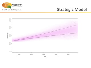
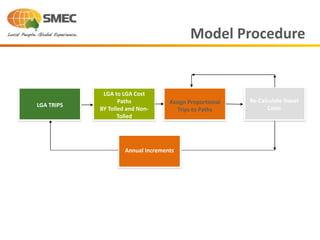
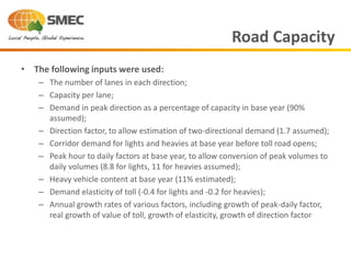
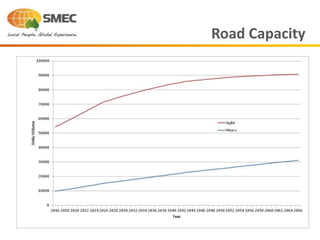
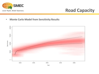
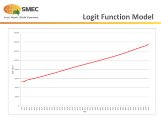
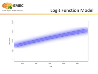
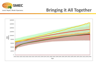
Multi-model forecasting provides more accurate forecasts than single models. The presentation discussed using multiple transportation demand models, including a strategic model, road capacity model, equilibrium model, and logit choice model. Key steps were to test sensitivity of inputs, develop Monte Carlo simulations of 10,000 observations to evaluate a 90% confidence interval, and average forecasts from multiple models. The approach emphasizes understanding complex interactions influencing forecasts and providing alternative outcome scenarios to help decision making for toll road projects.

1. Multi Model Forecasting
Presenter: Tony Fransos
Thursday 14 August 2014

2. Multi Model Forecasting
“The Commanding General is well aware that the
forecasts are no good. However, he needs them for
planning purposes.”
Memo to Ken Arrow after his warnings on the
unreliability of forecasts.

3. Reporting the Weather

4. The Aftermath
AFTERBEFORE

5. • New CRAY supercomputer
• Development of New Model Code
• Got it Right in Jan 1990
– But only because of 1 insistent meteorologist
• Moved to Ensemble Forecasting
– No storms missed since
– Can forecast storm 4 days in advance
The Remedy

6. • Flyvberg – We’re criminals
• Standard and Poors – forecasts are highly biased (at least 30% high)
• Robert Bain – We’ve deceived our clients
Transport Committee - Fifteenth Report
Better roads: Improving England's Strategic Road Network
• “building big new roads based on "black box" traffic forecasts is the wrong
way to go.”
• Department for Transport's (DfT) traffic projections form the basis of
the department's road building plans but have been shown up as
consistently and often dramatically inaccurate.
• hardly anyone knows how the DfT's models get it so wrong because there is
no proper scrutiny of them.
Our Michael Fish Moment

7. Our Michael Fish Moment

8. • “The best contribution that transport planners older than 50 can make to
the industry
• Is to retire and pass the torch to younger planners who might think more
openly”
Professor John Stanley
At a very pessimistic ITE seminar on Melbourne’s new Integrated Transport
Plan
Our Michael Fish Moment

9. Too often:
• The decision to provide infrastructure is political;
• Transport modelling is only used to justify the political decision
High forecasts have won all tenders for toll roads in Australia
The Problem with
Current Procedures
We really can't forecast all that well and yet we pretend that we can, but we
really can't.
Alan Greenspan

10. Submission to Infrastructure Australia’s Symposium into Traffic Forecasting
for Toll Roads
“The real issue here is that it if a developer wants to take an optimistic view of the future and ask
his traffic advisor to prepare forecasts on the basis of these optimistic assumptions, it is not the
fault of the advisor that the forecasts are ‘high’”.
The Problem with Us
Flyvbjerg
“… planners lie with numbers. Planners on the dark side are busy, not with getting forecasts
right and following an ethical path, but with getting projects funded and built. The most
effective planner is sometimes the one who can cloak advocacy in the guise of scientific or
technical rationality.”
Bain
“To knowingly inflate traffic and revenue projections is an act of deception – but it is
not alone in that regard. Investors reviewing toll road studies should remain alert to
two other potential acts of deceit.”

11. • Models don’t forecast, predict or estimate. Modellers do.
• Models Used/Abused to inflate forecasts
• Models not understood properly
• Models not explained properly
• Regarded as “black boxes”
Credibility of Transport Models

12. • Looking for a Practitioner’s Remedy
• Forecasts are not just reasonable but SEEN to be reasonable
• Provides alternative outcomes forecasting
• Understand the mechanics of the different models in order to forecast
successfully
• a way to understand more deeply the complex interactions that contribute
to transport demand in the future
Moving Forward
Forecasting with Multiple Models
“If you have to forecast, forecast often.”
Edgar Fiedler

13. • Even straight averages of forecasts from multiple models provide more
accurate forecasts than single individual models
• Multiple modelling need not require expensive solutions
• Basic assumptions and a small set of rules
• Liberal use of Monte Carlo Simulation to bolster understanding of risk
Moving Forward
Forecasting with Multiple Models

14. SMEC Study : Multi Model Forecast
Banora Point Upgrade, New South Wales, Australia

15. • Current 2 Lane Road
• 6-Lane Toll Road
• 2x 4 Lane competing arterials
• Start with A Strategic Model
• Test Sensitivity and Develop Monte Carlo Sim
Case Study
Non-toll
Lanes=10
Length=Ln
Speed=Sn
Capacity = 10*Cn
Toll
Lanes=6
Length=Lt
Speed=St
Capacity = 6*Ct

16. • The forecast volumes using the road tested to +10% and -10% changes to:
– The value of time;
– Price of fuel (part of the vehicle operating cost);
– Public transport fares;
– Population growth;
– Employment growth;
– Toll value.
• Monte Carlo simulation model
– 10,000 observations/tests
– Evaluated 90% confidence
Strategic Model

17. Strategic Model

18. Model Procedure
Name
Position
Name
Position
Name
Position
Assign Proportional
Trips to Paths
LGA Trips (AM Peak)
LGA to LGA Cost
Paths
BY Tolled and Non-
Tolled
LGA TRIPS
Re-Calculate Travel
Costs
Annual Increments

19. • The following inputs were used:
– The number of lanes in each direction;
– Capacity per lane;
– Demand in peak direction as a percentage of capacity in base year (90%
assumed);
– Direction factor, to allow estimation of two-directional demand (1.7 assumed);
– Corridor demand for lights and heavies at base year before toll road opens;
– Peak hour to daily factors at base year, to allow conversion of peak volumes to
daily volumes (8.8 for lights, 11 for heavies assumed);
– Heavy vehicle content at base year (11% estimated);
– Demand elasticity of toll (-0.4 for lights and -0.2 for heavies);
– Annual growth rates of various factors, including growth of peak-daily factor,
real growth of value of toll, growth of elasticity, growth of direction factor
Road Capacity

20. Road Capacity

21. • Monte Carlo Model from Sensitivity Results
Road Capacity

22. • Tolled route and untolled routes end up with equal travel costs
• Travel time calculated with volume-delay functions from strategic model
• Initial inputs and assumptions include:
– The free flow speeds on the toll road and competing routes;
– The length of the tolled route and competing routes;
– The number of lanes on the toll road and competing routes;
– The capacity per lane on the toll road and competing routes;
– The value of the toll;
– Directional and daily factors;
– A value of time;
– A vehicle operating cost converted to a time penalty by value of time;
– The toll was converted to a time penalty with an estimated value of time.
Equilibrium Model

23. Equilibrium Model

24. Equilibrium Model

25. • The utility function was a simple difference in the total costs (of travel
time, travel distance and toll) between the tolled route and its alternatives
• Binary choice logit model
• Inputs were taken from the strategic model where possible and include:
– The free flow speeds on the toll road and competing routes;
– The length of the tolled route and competing routes;
– The number of lanes on the toll road and competing routes;
– The capacity per lane on the toll road and competing routes;
– The value of the toll;
– Directional and daily factors;
– A value of time;
– A vehicle operating cost converted to time;
– The toll was converted to a time penalty with an estimated value of time.
Logit Choice Model

26. Logit Function Model

27. Logit Function Model

28. Bringing it All Together
“Far better an approximate answer to the right question, which is often vague, than
an exact answer to the wrong question, which can always be made precise.”
John W Tukey

29. Bringing it All Together

30. • Emphasises the importance of the planner ;
• Reduces the importance of individual models;
• Alternative outcomes of the models;
• The complex issues in involved with toll or patronage forecasting can be
examined in more depth and the issues understood;
• A tool to help make decisions about the way forecasts represent
interactions.
Conclusion
“He who lives by the crystal ball soon learns to eat ground glass.”
Edgar Fiedler