Downloaded 34 times


![Getting Outputs
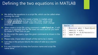
Use the following command in the Command Window
to get the outputs.
First code calls func1 and gives the outputs value
matrix [t, x].
Under the ode45() code, [0 10] gives time of run i.e. 0
to 10 seconds and [7 4.3] gives initial conditions of
𝑥1 (0) = 7 and 𝑥1(0) = 4.3.
Subplot() command is used to create multiple plots in
the same figure.
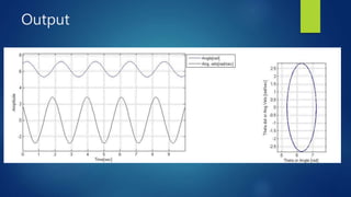
Third code gives the graph for time vs displacement of
the bob.
Hold on code is used to plot two
plots in one graph.
xlabel and ylabel codes are use to
label the axes in the graph.
Second last code gives the phase
trajectory for the pendulum.](https://image.slidesharecdn.com/analysingsimplependulumusingmatlab-170407193245/85/Analysing-simple-pendulum-using-matlab-5-320.jpg)


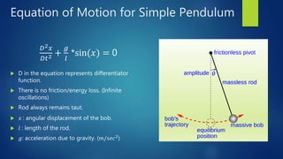
This document describes how to analyze a simple pendulum using MATLAB. It contains the equation of motion for a simple pendulum, notes on defining the equation in MATLAB, instructions for defining the two equations in a script file in MATLAB, and commands for running the code to output graphs of displacement over time and a phase trajectory plot.