The document is a lecture on MATLAB for automatic control systems, introducing its basic operations, matrix manipulations, and important functions for modeling and analyzing systems. It covers various model representations such as transfer function, zero-pole-gain, and state space, as well as stability and time/frequency domain analyses. Additionally, it outlines how to create and manage MATLAB files and includes examples of generating plots.

1. 1
ECEN 4413 - Automatic Control Systems
Matlab Lecture 1
Introduction and Control Basics
Presented by Moayed Daneshyari
OKLAHOMA STATE UNIVERSITY

2. 2
What is Matlab?
• Invented by Cleve Moler in late 1970s to give
students access to LINPACK and EISPACK
without having to learn Fortran.
• Together with Jack Little and Steve Bangert
they founded Mathworks in 1984 and created
Matlab.
• The current version is 7.
• Interpreted-code based system in which the
fundamental element is a matrix.

3. 3
The Interface
Workspace
and
Launch Pad
Command
History
and
Current
Directory
Command
Window

4. 4
 
  
 
1 2
m
3 4
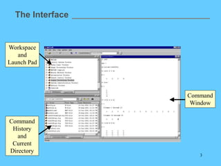
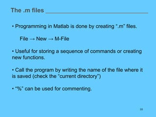
Variable assignment
• Scalar: a = 4
• Vector: v = [3 5 1]
v(2) = 8
t = [0:0.1:5]
• Matrix: m = [1 2 ; 3 4]
m(1,2)=0
 

v 3 5 1
 

v 3 8 1
 

t 0 0.1 0.2 4.9 5
 
  
 
1 0
m
3 4

5. 5
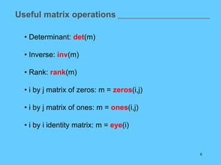
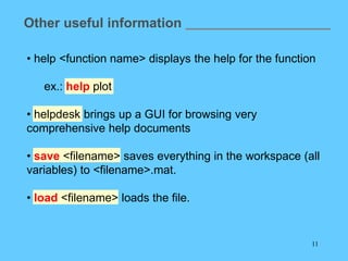
Basic Operations
• Scalar expressions
b = 10 / ( sqrt(a) + 3 )
c = cos (b * pi)
• Matrix expressions
n = m * [1 0]’


10
b
a 3
     
 
     
     
1 0 1 1
n
3 4 0 3


c cos(b )

6. 6
Useful matrix operations
• Determinant: det(m)
• Inverse: inv(m)
• Rank: rank(m)
• i by j matrix of zeros: m = zeros(i,j)
• i by j matrix of ones: m = ones(i,j)
• i by i identity matrix: m = eye(i)

7. 7
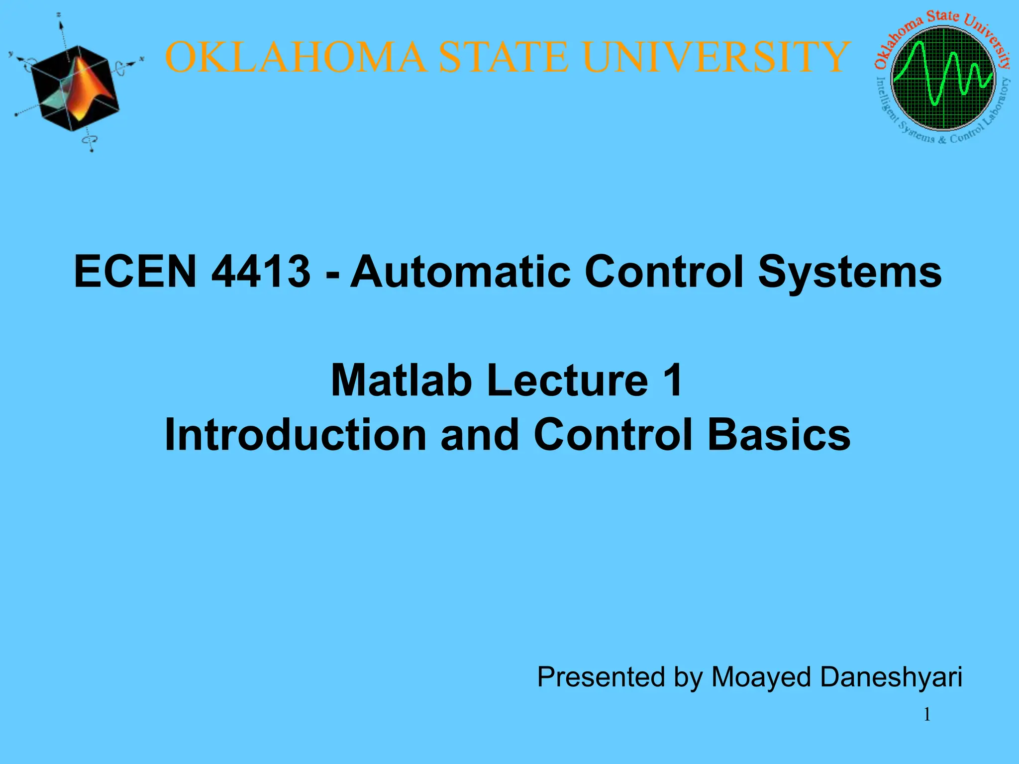
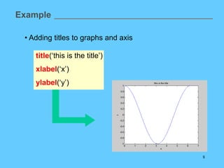
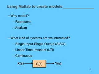
Example
• Generate and plot a cosine function
x = [0:0.01:2*pi];
y = cos(x);
plot(x,y)

8. 8
Example
• Adding titles to graphs and axis
title(‘this is the title’)
xlabel(‘x’)
ylabel(‘y’)

9. 9
Adding graphs to reports
• Three options:
1) Print the figure directly
2) Save it to a JPG / BMP / TIFF file and add to the
report (File → Export…)
3) Copy to clipboard and paste to the report
(Edit → Copy Figure) *
* The background is copied too! By default it is gray. To change the
background color use:
set(gcf,’color’,’white’)

10. 10
The .m files
• Programming in Matlab is done by creating “.m” files.
File → New → M-File
• Useful for storing a sequence of commands or creating
new functions.
• Call the program by writing the name of the file where it
is saved (check the “current directory”)
• “%” can be used for commenting.

11. 11
Other useful information
• help <function name> displays the help for the function
ex.: help plot
• helpdesk brings up a GUI for browsing very
comprehensive help documents
• save <filename> saves everything in the workspace (all
variables) to <filename>.mat.
• load <filename> loads the file.

12. 12
Using Matlab to create models
• Why model?
- Represent
- Analyze
• What kind of systems are we interested?
- Single-Input-Single-Output (SISO)
- Linear Time Invariant (LTI)
- Continuous
G(s) Y(s)
X(s)

13. 13
Model representations
Three Basic types of model representations for
continuous LTI systems:
• Transfer Function representation (TF)
• Zero-Pole-Gain representation (ZPK)
• State Space representation (SS)
! More help is available for each model representation by typing:
help ltimodels

14. 14
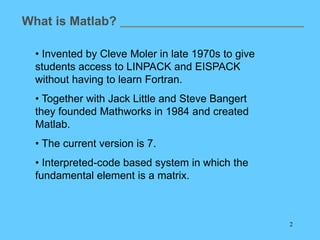
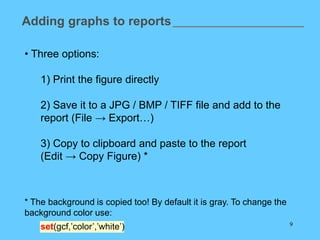
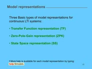
Transfer Function representation
Given:  
 
2
( ) 25
( )
( ) 4 25
Y s
G s
U s s s
num = [0 0 25];
den = [1 4 25];
G = tf(num,den)
Method (a) Method (b)
s = tf('s');
G = 25/(s^2 +4*s +25)
Matlab function: tf

15. 15
Zero-Pole-Gain representation
Given:

 
   
( ) 3( 1)
( )
( ) ( 2 )( 2 )
Y s s
H s
U s s i s i
zeros = [1];
poles = [2-i 2+i];
gain = 3;
H = zpk(zeros,poles,gain)
Matlab function: zpk

16. 16
State Space representation
Given: ,
 


 

x Ax Bu
y Cx Du
Matlab function: ss
   
   
 
   

   
  
1 0 1
2 1 0
3 2 0
A B
C D
A = [1 0 ; -2 1];
B = [1 0]’;
C = [3 -2];
D = [0];
sys = ss(A,B,C,D)

17. 17
System analysis
• Once a model has been introduced in Matlab, we can
use a series of functions to analyze the system.
• Key analyses at our disposal:
1) Stability analysis
e.g. pole placement
2) Time domain analysis
e.g. response to different inputs
3) Frequency domain analysis
e.g. bode plot

18. 18
Is the system stable?
Recall: All poles of the system must be on the right
hand side of the S plain for continuous LTI systems to
be stable.
Manually: Poles are the roots for the denominator
of transfer functions or eigen values of matrix A
for state space representations
In Matlab: pole(sys)
Stability analysis

19. 19
Once a model has been inserted in Matlab, the step
response can be obtained directly from: step(sys)
Time domain analysis
Unit Step Response of G(s)
Time (sec)
Amplitude
0 0.5 1 1.5 2 2.5 3
0.2
0.4
0.6
0.8
1
1.2
1.4
Peak Time
Rise Time
Steady State
Settling Time
overshoot

20. 20
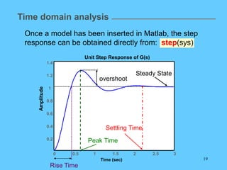
Time domain analysis
• Impulse response
impulse(sys)
• Response to an arbitrary input
e.g.
t = [0:0.01:10];
u = cos(t);
lsim(sys,u,t)
Matlab also caries other useful functions for time domain
analysis:
! It is also possible to assign a variable to those functions to obtain a
vector with the output. For example: y = impulse(sys);

21. 21
Bode plots can be created directly by using: bode(sys)
Frequency domain analysis

22. 22
For a pole and zero plot: pzmap(sys)
Frequency domain analysis
-2 -1.8 -1.6 -1.4 -1.2 -1 -0.8 -0.6 -0.4 -0.2 0
-4
-3
-2
-1
0
1
2
3
4
Pole-Zero Map
Real Axis
Imaginary
Axis

23. 23
Extra: partial fraction expansion
num=[2 3 2];
den=[1 3 2];
[r,p,k] = residue(num,den)
r =
-4
1
p =
-2
-1
k =
2
Answer:
)
1
(
1
)
2
(
4
2
)
(
)
(
)
1
(
)
1
(
)
(
)
(
0














s
s
s
n
p
s
n
r
p
s
r
s
k
s
G 

2
3
2
3
2
)
( 2
2





s
s
s
s
s
G
Given: