This document discusses modeling dynamic systems using MATLAB/Simulink. It provides examples of creating simple programs in MATLAB to solve equations and modeling the same programs in Simulink. It also discusses modeling a nonlinear pendulum system using different Simulink blocks, including individual blocks, state-space models, and transfer functions. Finally, it covers linearizing nonlinear systems and using the linearization tool in MATLAB to analyze systems.

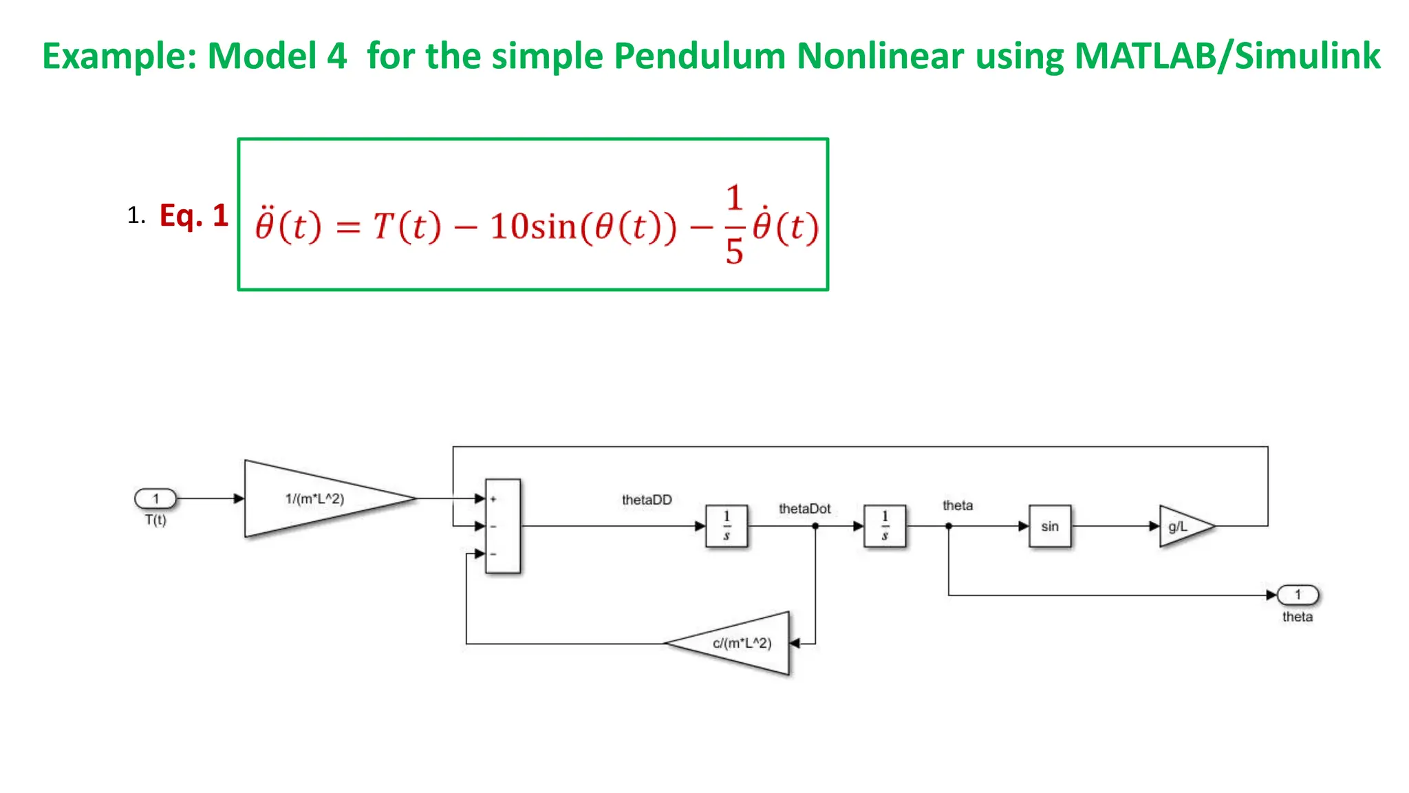
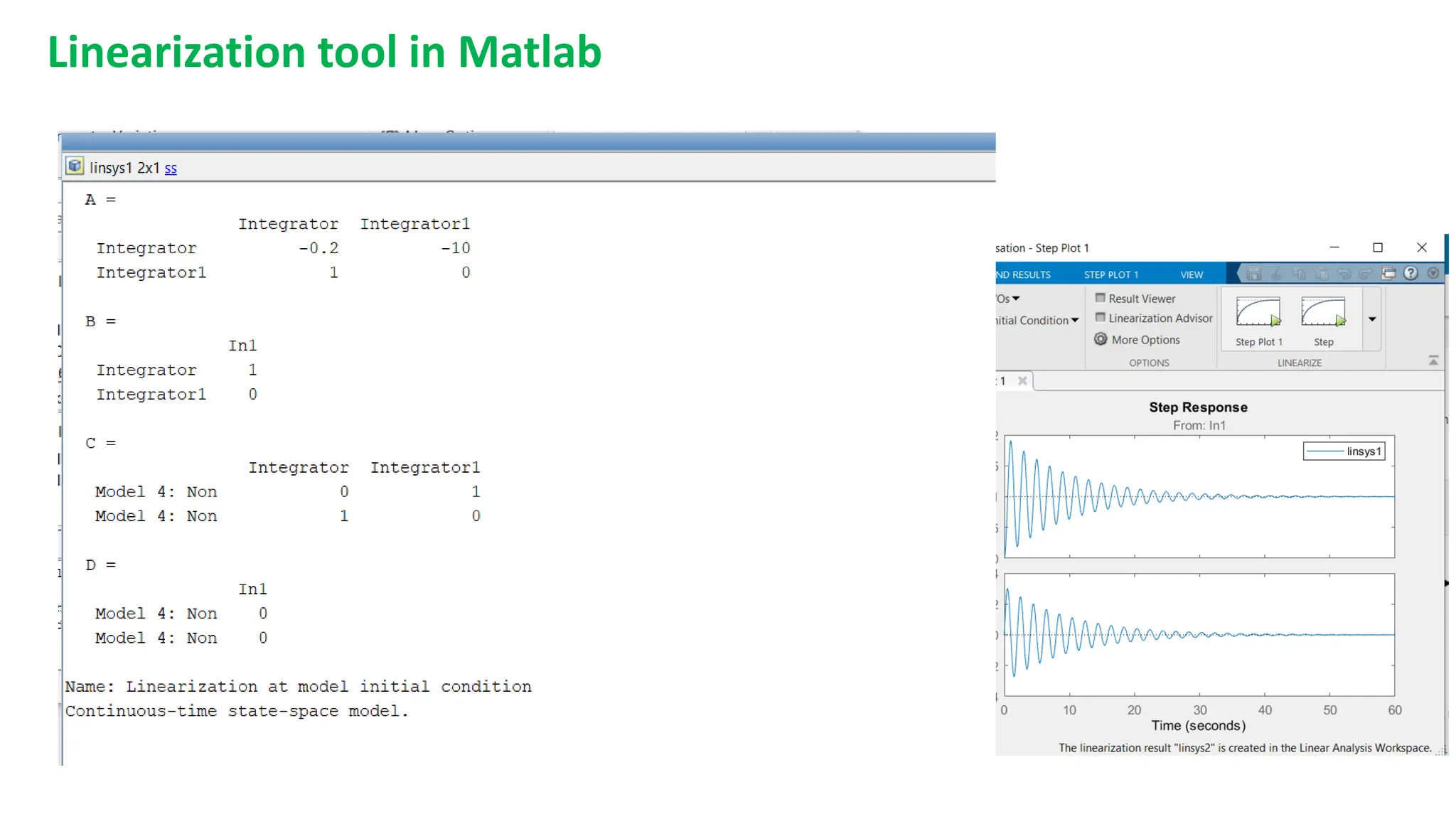
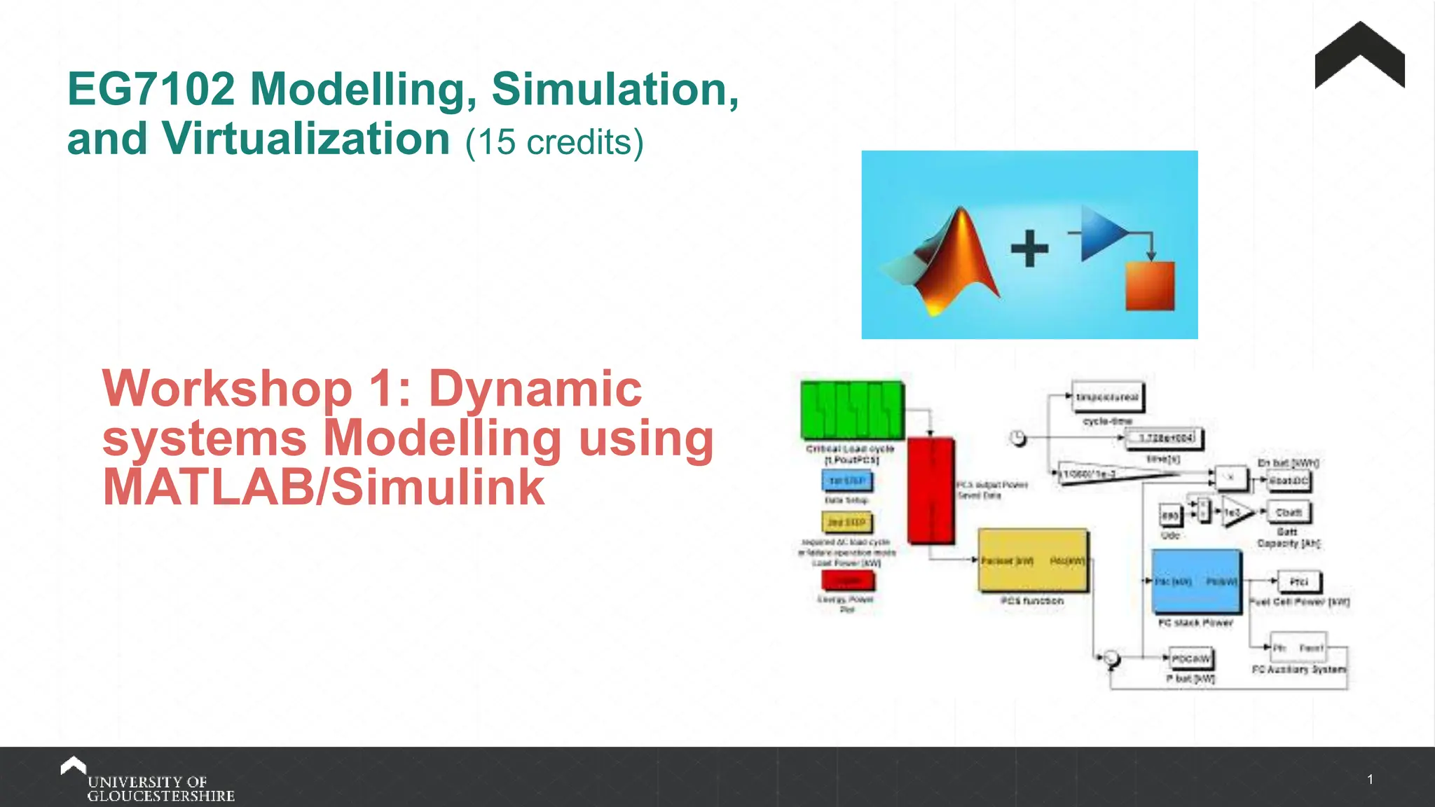
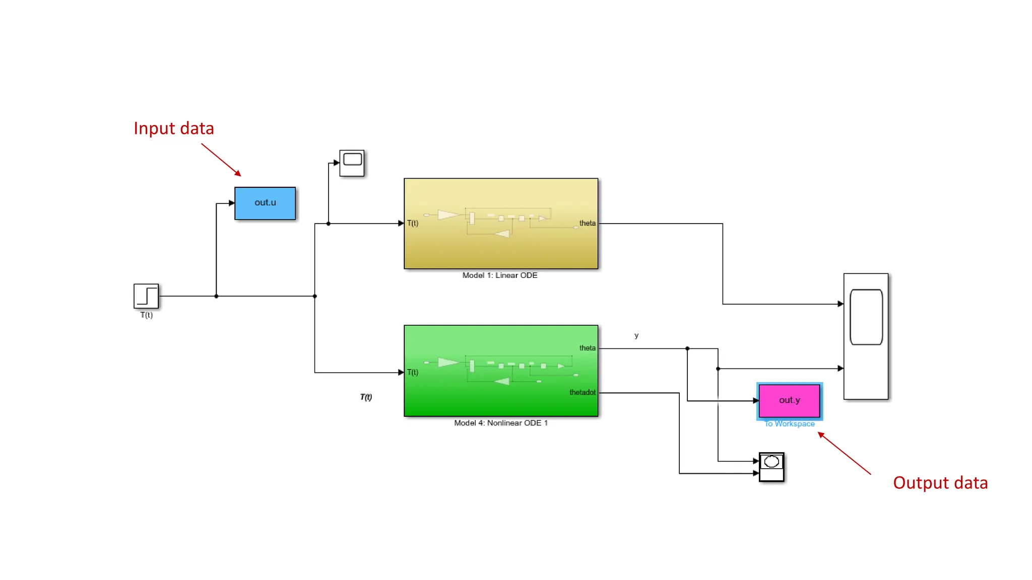
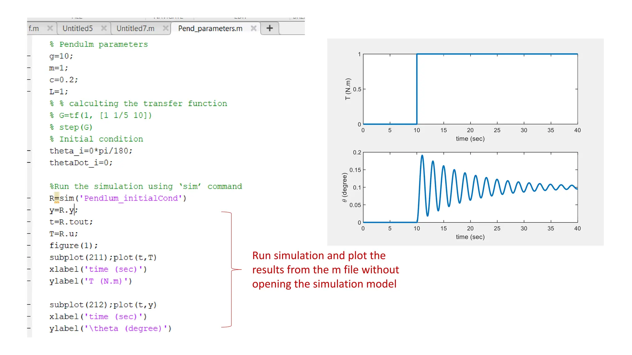
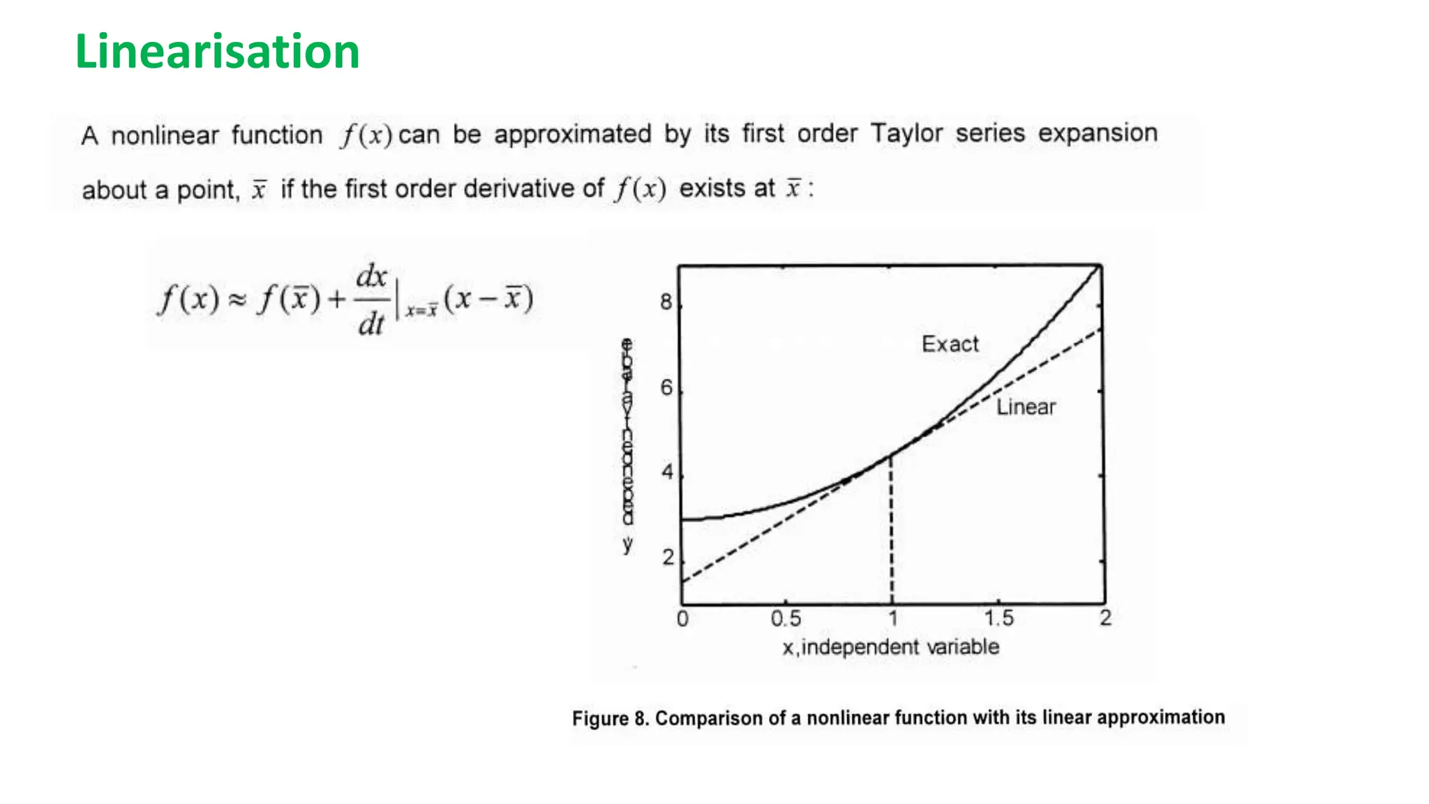
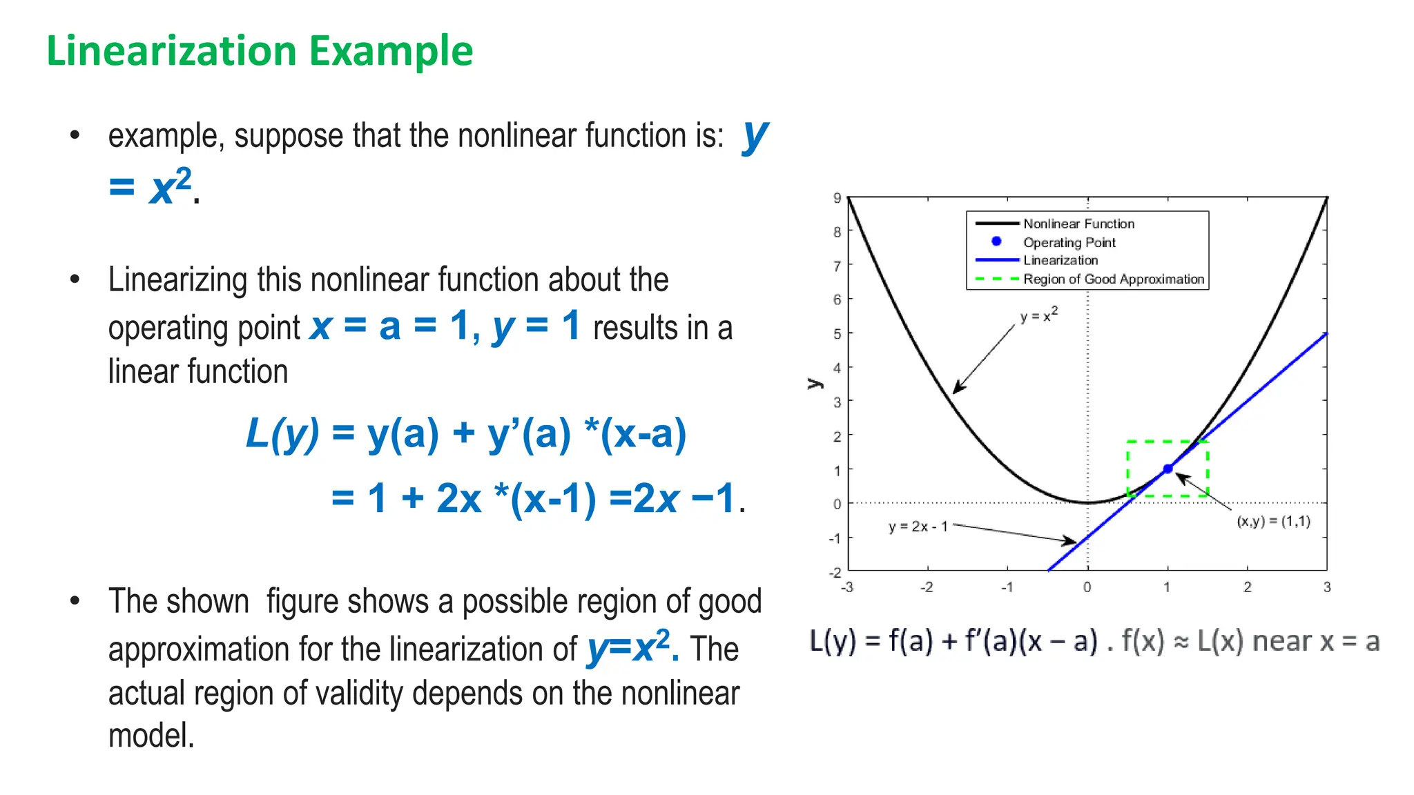
1. 1
EG7102 Modelling, Simulation,
and Virtualization (15 credits)
Workshop 1: Dynamic
systems Modelling using
MATLAB/Simulink

2. Outline
1.What is Simulink?
2.Creating a simple program in MATLAB
3.Creating an equivalent program in SIMULINK

3. 1. Creating a simple program to solve Algebra equations in MATLAB
Example: Find the value of q in the following equation.
(1)
(2)
(3)

4. Step 1: Create function for f(x)
Method 1: Creating functions and using MATLAB functions to find the value of q
Equation 1

5. Step 2: Create function for h(p,w)
Equation 2

6. Step 3: Call the functions f(x) & h(w,p) to find the value of q

7. Results

8. We can acssess to Simulink by two ways
1. type Simulink in the workspace
2. Click the Simulink icon in the upper bar
Method 2: Using MATLAB/Simulink to find the value of q

10. New Simulation model
SIMULINK Library
Method 1: Creating functions and using MATLAB codes to find the value of q

11. Finding the value of variable q using MATLAB/Simulink blocks

12. Finding the value of variable q using MATLAB/Simulink blocks

13. Finding the value of variable q using Matlab/Simulink with subsystem blocks
Subsystem 1
Subsystem 2

14. 1. Develop a differential equation describing the dynamics
of a nonlinear system.
2. Investigate various methods in Simulink to solve these
systems (individual blocks, state space, and transfer
functions).
3. Simulate the response of these systems to inputs and
initial conditions.
4. Modify the system to include nonlinear dynamics.
2. Solving ODEs using MATLAB/SIMULINK toolbox

15. Example: Equations of motion: The simple Pendulum
The ODE describes the dynamic response
2n-order system
Nonlinear because we have sin()
J 𝜃 𝑡 = 𝑇 𝑡 − 𝑚𝑔𝐿 sin 𝜃 𝑡 − 𝑐𝜃 𝑡
𝜃 𝑡 =
1
𝐽
𝑇 𝑡 −
𝑚𝑔𝐿
𝐽
sin 𝜃 𝑡 −
𝑐
𝐽
𝜃 𝑡
Re-arrange the above equation:
𝐽 = 𝑚𝐿2
Recall
𝜃 𝑡 =
1
𝑚𝐿2
𝑇 𝑡 −
𝑔
𝐿
sin(𝜃 𝑡 ) −
𝑐
𝑚𝐿2
𝜃(𝑡) Eq. 1

16. The ODE describes the dynamic response of the Pendulum
For initial condition  = 0o
we can approximate the above nonlinear ODE to
linear (Eq. 2) because Sin() = 0 = 
Eq. 1
Eq. 2
𝜃 𝑡 =
1
𝑚𝐿2
𝑇 𝑡 −
𝑔
𝐿
𝜃 𝑡 −
𝑐
𝑚𝐿2
𝜃(𝑡)
𝜃 𝑡 =
1
𝑚𝐿2
𝑇 𝑡 −
𝑔
𝐿
sin(𝜃 𝑡 ) −
𝑐
𝑚𝐿2
𝜃(𝑡)
The new model will be linear
The nonlinear model

17. Assume the values of the system parameters (constants) as given below;
g = 10 m/s2
m = 1 kg
c = 0.2 Nm/rad/sec
L = 1m
1/mL2 = 1;
g/L =10;
c/mL2 = 1/5
Eq. 1
Eq. 2
Nonlinear for any value
of initial
Linear when initial = 0o

18. The simple pendulum model (final)
Pendulum
Model
Input
T, Torque Output
, the deflection
angle
g = 10 m/s2
m = 1 kg
c = 0.2 Nm/rad/sec
L = 1m
T(t ),  (t) : Model variables
Model
parameters

19. Model 1: using MATLAB/SIMULINK individual blocks
1. Create m file to define the model parameters (constants)

20. 2. Run the previous m file to generate the model parameters in the workspace
3. Build the Simulink model as shown below and you should get the shown results

21. Model 2: using state-space model via MATLAB/SIMULINK
Let 𝑥1 = 𝜃
𝑥2 = 𝜃
A
Eq. 3
Eq. 4
B
C D

22. Method 2: using state-space model via MATLAB/SIMULINK
A B
C D
g = 10 m/s2; m = 1 kg; c = 0.2 Nm/rad/sec;
L = 1m
Substituting the parameters values in Eq 3 and 4 yields
Eq. 3
Eg. 4

23. State-space model

24. Model 3: using transfer function model via MATLAB/SIMULINK
Take Laplase transform for both sides of Eq. 2
Eq. 2
𝜃 𝑡 =
1
𝑚𝐿2
𝑇 𝑡 −
𝑐
𝑚𝐿2
𝜃 𝑡 −
𝑔
𝐿
𝜃(𝑡)
L { }
𝑠2𝜽(𝑠 =
1
𝑚𝐿2
𝑻 𝑠 −
𝑐
𝑚𝐿2
𝑠𝜽(𝑠) −
𝑔
𝐿
𝜽(𝑠)
𝑠2
𝜽 𝑠 +
𝑐
𝑚𝐿2
𝑠𝜽 𝑠 +
𝑔
𝐿
𝜽(𝑠) =
1
𝑚𝐿2
𝑻 𝑠
𝒔2 +
𝑐
𝑚𝐿2
𝒔 +
𝑔
𝐿
𝜽(𝑠) =
1
𝑚𝐿2
𝑻(s)
… continue

25. T.F = G(s) =
𝑶𝒖𝒕𝒑𝒖𝒕
𝑰𝒏𝒑𝒖𝒕
For: g = 10 m/s2; m = 1 kg; c = 0.2 Nm/rad/sec; L = 1m 1/mL2 = 1;
g/L =10;
c/mL2 = 1/5
∴ G 𝒔 =
𝜽(𝒔)
𝑻(𝒔)
=
1/𝑚𝐿2
𝑠2 +
𝑐
𝑚𝐿2 𝑠 +
𝑔
𝐿
Eq. 5
G 𝒔 =
𝜽(𝒔)
𝑻(𝒔)
=
1
𝑠2 +
1
5
𝑠 + 10 Eq. 6
Transfer
function

26. • Model 3: using transfer function model via code in MATLAB
1.

27. • Model 3: using transfer function model using MATLAB/Simulink
1.

28. • Model 4: Nonlinear ODE (Eq. 1) using MATLAB/Simulink
1. Eq. 1

29. • Model 4: Nonlinear ODE (Eq. 1) using MATLAB/Simulink (i = 0 degree)
i = 0 degree

30. Increasing the damping, c=0.5
i = 0 degree

31. T(t)
Unit Step function at t=5 sec, T(t)= 1
 (t) step response using four models
for initial condition i = 0 degree
Increasing the
damping, c = 0.5

32. • Model 4: Nonlinear ODE (Eq. 1) using MATLAB/Simulink (i = 0 degree)
i = 45 degree
https://upload.wikimedia.org/wikipedia/commons/c/c1/Pendu
lum_45deg.gif

33. i = 45 degree
i
Double
click

34. t =10 sec
Nonlinear ODE
i = 45 degree

35. i = 90 degree
Damping
parameter, c= 0.5

36. i = 180 degree
Damping parameter, c= 0.2
Linearized model frailer

37. Increasing the rod length to 6 m = Increasing the settling time

38. Adding X-Y plotter block to plot theta versus thetaDot

39. Theta
Theta dot
Adding X-Y plotter block to plot theta versus thetaDot

41. 3. Extract simulation results in the work space

42. Change name to y
Change save format to Array
Extract simulation results in the work space

43. Extract simulation results in the work space

44. Output data
Input data

45. Run simulation and plot the
results from the m file without
opening the simulation model

46. Linearisation

47. Linearization Example
• example, suppose that the nonlinear function is: y
= x2.
• Linearizing this nonlinear function about the
operating point x = a = 1, y = 1 results in a
linear function
L(y) = y(a) + y’(a) *(x-a)
= 1 + 2x *(x-1) =2x −1.
• The shown figure shows a possible region of good
approximation for the linearization of y=x2. The
actual region of validity depends on the nonlinear
model.

49. • Linear State space model
• Nonlinear State space model
• The steady-state equations for the above system are
(2)
(1)

50. (2)
Jacobian matrix
State Space Linearization
(1)

51. 2x1 cos(x2)
0 -3(x2)2
x1=1,x2=0
=
2 1
0 0
A = B =
0
1 C = [1 1], D = 0
;
;
Solution:

52. Example: Model 4 for the simple Pendulum Nonlinear using MATLAB/Simulink
1. Eq. 1

53. Linearization tool in Matlab
Compute Open-Loop Response Using Model Linearizer
1.Open the Linearization tab. To do so, in the Apps gallery,
click Linearization Manager.
2. To specify an analysis point for a signal, click the signal in the
model. Then, on the Linearization tab, in the Insert Analysis
Points gallery, select the type of analysis point.
3. Configure the input signal of the input of the block as an Input
Perturbation.
4. Configure the output signal of the output of the block
5. System block as an Open-loop Output.
Annotations appear in the model indicating which signals are
designated as analysis points. T
theta

54. Linearization tool in Matlab
• Click on Step plot 1
• The steady-state model will
appear in the Linear Analysis
Workspace
• Double click on ‘linsys1’

55. 1. Equations of motion for an example dynamic system
2. Implementing linear ODE
a) Individual blocks
b) State space
c) Transfer function
3. Simulating response of the system
a) inputs
b) Intial condition
c) Run the simulation model from the m.file
d) Extracting and plotting the simulation results from the m.file
Summery

56. Questions