Download as PDF, PPTX


![Centre Tecnològic de Telecomunicacions de Catalunya - CTTC
Parc Mediterrani de la Tecnologia, Castelldefels (Barcelona), Spain, http://www.cttc.cat/
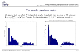
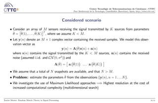
The sample covariance matrix
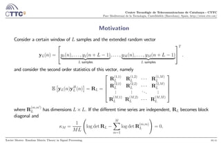
We assume that we collect independent samples (snapshots) from an array of antennas:
Consider the × observation matrix Y = [y(1) y()] and the sample covariance matrix
ˆR =
1
YY
=
1
X
=1
y()y
()
Xavier Mestre: Random Matrix Theory in Signal Processing. 3/41](https://image.slidesharecdn.com/presentationklagenfurt-190305105501/85/Random-Matrix-Theory-in-Array-Signal-Processing-Application-Examples-3-320.jpg)

![Centre Tecnològic de Telecomunicacions de Catalunya - CTTC
Parc Mediterrani de la Tecnologia, Castelldefels (Barcelona), Spain, http://www.cttc.cat/
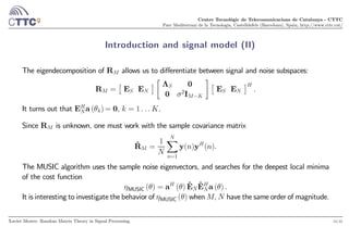
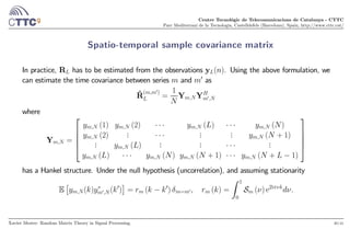
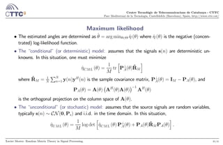
Conditional versus unconditional model (II)
Depending on how the signals are modeled, we differentiate between the conditional and the
unconditional models. Let us denote
S = [s(1) s()]
• Conditional Model: The entries of S are modelled as deterministic unknowns. In this case, the
observation can be described as
y() ∼ CN
¡
A (Θ) s() 2
I
¢
• Unconditional Model: The entries of S are modelled as random variables. Typically, we assume
that the column vectors s() are independent, circularly symmetric Gaussian Random variables, i.e.
s ∼ CN (0 P), P 0. In this case, we have
y() ∼ CN (0 R) R = A (Θ) PA
(Θ) + 2
I
Xavier Mestre: Random Matrix Theory in Signal Processing. 6/41](https://image.slidesharecdn.com/presentationklagenfurt-190305105501/85/Random-Matrix-Theory-in-Array-Signal-Processing-Application-Examples-6-320.jpg)
![Centre Tecnològic de Telecomunicacions de Catalunya - CTTC
Parc Mediterrani de la Tecnologia, Castelldefels (Barcelona), Spain, http://www.cttc.cat/
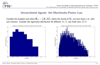
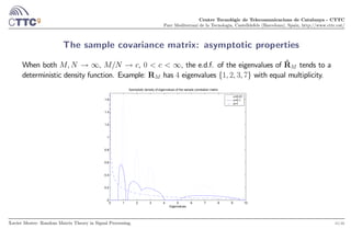
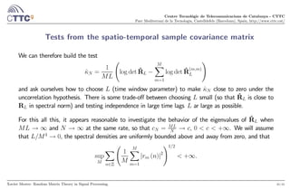
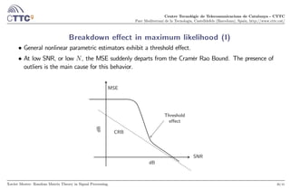
Uncorrelated signals: the Marchenko-Pastur Law (II)
It turns out, that when → ∞, → , 0 ∞, the empirical density of eigenvalues
converges to a deterministic measure.
0.4 0.6 0.8 1 1.2 1.4 1.6 1.8 2
0
2
4
6
8
10
12
14
Eigenvalues
Histogram of the eigenvalues of the sample covariance matrix, M=800, N=8000
Numberofeigenvalues
For 1 () = 1
2
q¡
− −
¢ ¡
+
−
¢
I[−
+
]() −
= (1 −
√
)
2
+
= (1 +
√
)
2
.
Xavier Mestre: Random Matrix Theory in Signal Processing. 9/41](https://image.slidesharecdn.com/presentationklagenfurt-190305105501/85/Random-Matrix-Theory-in-Array-Signal-Processing-Application-Examples-9-320.jpg)

![Centre Tecnològic de Telecomunicacions de Catalunya - CTTC
Parc Mediterrani de la Tecnologia, Castelldefels (Barcelona), Spain, http://www.cttc.cat/
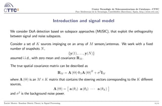
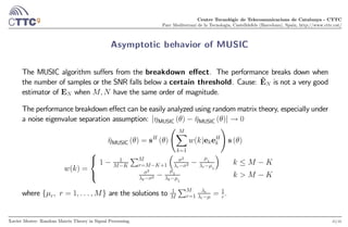
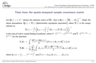
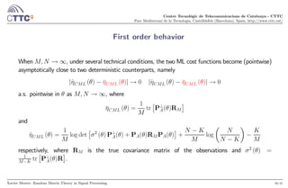
Asymptotic behavior of MUSIC: an example
We consider a scenario with two sources impinging on a ULA ( = 05, = 20) from DoAs:
35◦
, 37◦
.
−100 −80 −60 −40 −20 0 20 40 60 80 100
−35
−30
−25
−20
−15
−10
−5
0
MUSIC asymptotic pseudospectrum, M=20, DoAs=[35,37]deg
Azimuth (deg)
32 34 36 38 40
−32
−30
−28
−26
−24
−22
−20
−18
N=25
N=15
SNR=12dB
SNR=17dB
2 4 6 8 10 12 14 16 18 20
25
30
35
40
45
50
SNR (dB)
Azimuth(deg)
Position of the two deepest local minima of the asymptotic MUSIC cost function
10 12 14
35
36
37
N=15
N=25
Xavier Mestre: Random Matrix Theory in Signal Processing. 16/41](https://image.slidesharecdn.com/presentationklagenfurt-190305105501/85/Random-Matrix-Theory-in-Array-Signal-Processing-Application-Examples-16-320.jpg)


![Centre Tecnològic de Telecomunicacions de Catalunya - CTTC
Parc Mediterrani de la Tecnologia, Castelldefels (Barcelona), Spain, http://www.cttc.cat/
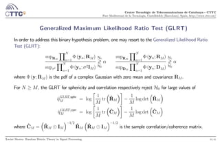
Introduction: testing independence of multiple time series
We consider an -variate zero-mean Gaussian time series
y() = [1() ()]
where = 1 , and ask ourselves whether the different components of the series are independent.
Xavier Mestre: Random Matrix Theory in Signal Processing. 28/41](https://image.slidesharecdn.com/presentationklagenfurt-190305105501/85/Random-Matrix-Theory-in-Array-Signal-Processing-Application-Examples-28-320.jpg)

![Centre Tecnològic de Telecomunicacions de Catalunya - CTTC
Parc Mediterrani de la Tecnologia, Castelldefels (Barcelona), Spain, http://www.cttc.cat/
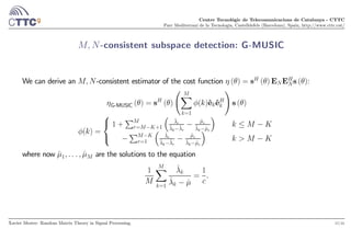
Breakdown effect in maximum likelihood (II)
At low values of the SNR and , there exist realizations of the cost functions for which local minima
corresponding to outliers become deeper than the intended one.
UML, SNR=0dB, M=5, N=20, uncorrelated signals,DoA=[16,18]deg
θ1
(deg)θ2
(deg)
−80 −60 −40 −20 0 20 40 60 80
−80
−60
−40
−20
0
20
40
60
80
UML cost function
Local Minima
Intended Minimum
Selected Minimum
Xavier Mestre: Random Matrix Theory in Signal Processing. 37/41](https://image.slidesharecdn.com/presentationklagenfurt-190305105501/85/Random-Matrix-Theory-in-Array-Signal-Processing-Application-Examples-37-320.jpg)
![Centre Tecnològic de Telecomunicacions de Catalunya - CTTC
Parc Mediterrani de la Tecnologia, Castelldefels (Barcelona), Spain, http://www.cttc.cat/
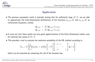
Probability of resolution
• We consider here the definition of [Athley, 05] of the resolution probability. If ˆ () is a generic cost
function that fluctuates around a deterministic ¯ (), which has + 1 local minima at the values
¯ 1 , the probability of resolution can be defined as
= P
"
=1
©
ˆ () ˆ
¡
¯
¢ª
#
• It was shown in [Athley, 05] that this definition of provides a very accurate description of both
the breakdown effect and the expected mean squared error (MSE) of the DoA estimation process.
• Unfortunately, in our ML setting, is difficult to analyze for finite values of due to the
complicated structure of the cost functions, especially ˆ ().
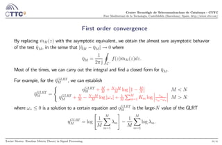
• We propose to use the asymptotic distributions (as → ∞) instead of the actual ones. Very
accurate description of the actual probability, even for very low .
Xavier Mestre: Random Matrix Theory in Signal Processing. 38/41](https://image.slidesharecdn.com/presentationklagenfurt-190305105501/85/Random-Matrix-Theory-in-Array-Signal-Processing-Application-Examples-38-320.jpg)
![Centre Tecnològic de Telecomunicacions de Catalunya - CTTC
Parc Mediterrani de la Tecnologia, Castelldefels (Barcelona), Spain, http://www.cttc.cat/
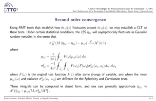
Second order behavior
Let 1 be a set of multidimensional points (e.g. local minima of ¯ () or ¯ ()). Let
ˆη = [ˆ (1) ˆ ()]
and ¯η = [¯ (1) ¯ ()]
and take the equivalent definitions for the UML cost function. Assume that y() ∼ CN (0 R).
Under certain technical conditions, as → ∞ , → , 0 1, we have
Γ−1
(ˆη − ¯η) → N (0 I) and Γ−1
(ˆη − ¯η) → N (0 I)
for some covariance matrices Γ, Γ given by
{Γ} =
1
tr
£
P⊥
P⊥
¤
and
{Γ} =
1
2
2
1
tr
£
P⊥
P⊥
¤
+
1
2
1
tr
£
P⊥
Q
¤
+
1
2
1
tr
£
P⊥
Q
¤
− log
¯
¯
¯
¯1 −
1
tr [QQ]
¯
¯
¯
¯
where P = R
12
P
³
()
´
R
12
,P⊥
= R − P, and Q = R
12
A
£
A
RA
¤−1
A
R
12
.
Xavier Mestre: Random Matrix Theory in Signal Processing. 40/41](https://image.slidesharecdn.com/presentationklagenfurt-190305105501/85/Random-Matrix-Theory-in-Array-Signal-Processing-Application-Examples-40-320.jpg)
![Centre Tecnològic de Telecomunicacions de Catalunya - CTTC
Parc Mediterrani de la Tecnologia, Castelldefels (Barcelona), Spain, http://www.cttc.cat/
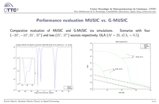
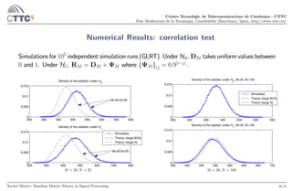
Simulation results
ULA of = 5 elements, two sources coming from 16 and 18 degrees with respect to the broadside.
−15 −10 −5 0 5 10 15 20 25
0.1
0.2
0.3
0.4
0.5
0.6
0.7
0.8
0.9
1
SNR (dB)
Prob.ofRes.
Prob. of res., M=5, Theta=[16,18] deg, corr=0
UML (Predicted)
UML (Simulated)
CML (Predicted)
CML (Simulated)
N=100
N=10
Uncorrelated sources
−15 −10 −5 0 5 10 15 20 25
0.1
0.2
0.3
0.4
0.5
0.6
0.7
0.8
0.9
1
SNR (dB)Prob.ofRes.
Prob. of res., M=5, Theta=[16,18] deg, corr=0.95
UML (Predicted)
UML (Simulated)
CML (Predicted)
CML (Simulated)
N=100
N=10
Highly correlated sources
Xavier Mestre: Random Matrix Theory in Signal Processing. 42/41](https://image.slidesharecdn.com/presentationklagenfurt-190305105501/85/Random-Matrix-Theory-in-Array-Signal-Processing-Application-Examples-42-320.jpg)

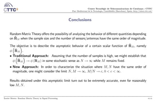


The document discusses the application of Random Matrix Theory (RMT) in signal processing, detailing how it enables convergence analysis of the sample covariance matrix under various conditions. It highlights multiple applications such as direction-of-arrival estimation, detection tests, multivariate time series analysis, and outlier characterization. The significance of understanding the asymptotic properties of eigenvalues in large dimensional settings is emphasized throughout the text.