Download to read offline

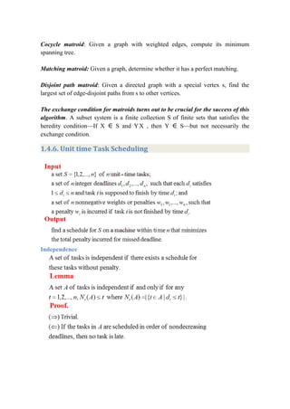
![Greedy Activity Selector Algorithm
Greedy-Activity-Selector(s, f)
1. n ← length[s]
2. A ← {a1}
3. i ← 1
4. for m ← 2 to n
5. do if sm ≥ fi
6. then A ← A U {am}
7. i ← m
8. return A
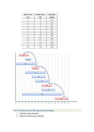
Example
Points to remember
For this algorithm we have a list of activities with their starting time
and finishing time.
Our goal is to select maximum number of non-conflicting activities that
can be performed by a person or a machine, assuming that the person or
machine involved can work on a single activity at a time.
Any two activities are said to be non-conflicting if starting time of one
activity is greater than or equal to the finishing time of the other
activity.
In order to solve this problem we first sort the activities as per their
finishing time in ascending order.
Then we select non-conflicting activities.
Problem
Consider the following 8 activities with their starting and finishing time.
Our goal is to find non-conflicting activities.
For this we follow the given steps
1. sort the activities as per finishing time in ascending order
2. select the first activity
3. select the new activity if its starting time is greater than or equal to the
previously selected activity
REPEAT step 3 till all activities are checked
Step 1: sort the activities as per finishing time in ascending order
Step 2: select the first activity
Step 3: select next activity whose start time is greater thanor equal to the finish
time of the previously selected activity](https://image.slidesharecdn.com/daachapter4-200419170136/85/Daa-chapter4-3-320.jpg)
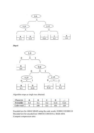

The document discusses greedy algorithms and matroids. It provides examples of problems that can be solved using greedy approaches, including sorting an array, the coin change problem, and activity selection. It defines key aspects of greedy algorithms like the greedy choice property and optimal substructure. Huffman coding is presented as an application that constructs optimal prefix codes. Finally, it introduces matroids as an abstract structure related to problems solvable by greedy methods.


![Lec 8 03_sept [compatibility mode]](https://cdn.slidesharecdn.com/ss_thumbnails/lec803septcompatibilitymode-130917013815-phpapp02-thumbnail.jpg?width=640&height=640&fit=bounds)