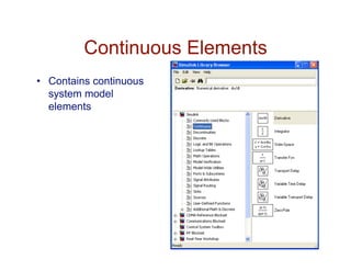
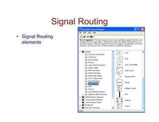
SlideShare a Scribd company logo
1 of 45
Download to read offline
MATLAB Simulink
What is Simulink
•  Simulink is an input/output device GUI block diagram
simulator.
•  Simulink contains a Library Editor of tools from which we
can build input/output devices and continuous and
discrete time model simulations.
•  To open Simulink, type in the MATLAB work space
–  >>simulink
The Library Editor
•  >>simulink
•  Simulink opens with
the Library Browser
•  Library Browser is
used to build
simulation models
Continuous Elements
•  Contains continuous
system model
elements
Discontinuous Elements
•  Contains
discontinuous system
model elements
Math Operations
•  Contains list of math
operation elements
Signal Routing
•  Signal Routing
elements
Sink Models
•  Sinks: sink device
elements. Used for
displaying simulation
results
Signal Routing
•  Sources: provides list of
source elements used for
model source functions.
Signal Routing
•  Simulink Extras: additional
linear provide added block
diagram models. The two
PID controller models are
especially useful for PID
controller simulation.
Building Models
•  Creating a New Model
•  To create a new model, click the New button on the
Library Browser’s toolbar
•  This opens a new untitled model window.
Building Models (2)
•  Model elements are added by selecting the appropriate
elements from the Library Browser and dragging them
into the Model window. Alternately, they may be copied
from the Library Browser and pasted into the model
window.
•  To illustrate lets model the capacitor charging equation:
Modeling the Capacitor System
Modeling the Capacitor System (2)
Unconnected system model
Connecting the System Blocks
System blocks are connected in to ways; one way is the auto
connect method which is done by 1st selecting the source block
and holding down the Cntr key and selecting the destination
block.
Simulink also allows you to draw lines manually between blocks
or between lines and blocks. To connect the output port of one
block to the input port of another block: Position the cursor over
the first block’s output port. The cursor shape changes to
crosshairs. Right click and drag the crosshairs to the input of the
destination block to make the connection.
The next slide shows the connected model
The Connected Capacitor Model
Connected system model
Editing the Capacitor Model
Now that we have connected the model, we need to edit it. This
is done by selecting and double clicking to open the appropriate
models and then editing. The blocks we need to edit are the
step function, the two gain blocks, and the summing junction
block.
Editing the Capacitor Model (2)
In editing the blocks note that we have set the height of the step
function at 10, left R and C as variable (we will enter these from
the workspace), and changed the sign of the summing junction
input from + to -.
Controlling the Simulation
Simulation control is fixed by
selecting Configuration
Parameters
Controlling the Simulation - Solver
Simulink uses numerical integration to solve dynamic system
equations. Solver is the engine used for numerical integration.
Key parameters are the Start and Stop times, and the Solver
Type and methods.
Solver Parameters
The Start and Stop times set the start and stop times for the
simulation.
Solver Type sets the method of numerical integration as variable
step or fixed step. Variable step continuously adjusts the
integration step size so as to speed up the simulation time.
I.E., variable step size reduces the step size when a model’s
states are changing rapidly to maintain accuracy and increases
the step size when the system’s states are changing slowly in
order to avoid taking unnecessary steps.
Fixed step uses the same fixed step size throughout the
simulation. When choosing fixed step it is necessary to set the
step size.
Setting Fixed Step Size
The following example illustrates setting the fixed step size to a
value of 0.01 seconds.
Setting Fixed Step Size
The following example illustrates setting the fixed step size to a
value of 0.01 seconds.
Setting the Integration Type
The list of integration type solvers are shown below. For more
information on fixed and variable step methods and integration
types consult the MATLAB Simulink tutorial.
Running the Simulation
To run the simulation we 1st need to enter the values of R and
C. Note we could have entered these directly in the gain blocks
but we chose to enter these from the work space. To do this in
the work space we type
>>R = 1; C = 1;
This will fix the gain block’s as K = 1/(R*C)
Now select and click
the run button to run
the simulation
Viewing the Simulation with the Scope
To view the simulation results double click on the Scope block to
get. To get a better view left click and select Autoscale
Setting the Scope Axis Properties
We can adjust the Scope axis properties to set the axis limits:
Setting the Scope Parameters
The default settings for the Scope is a Data History of 5000 data
samples. By selecting Parameters an un-clicking the Limit
data points to last 5000 we can display an unlimited number of
simulation samples. Especially useful for long simulations or
simulations with very small time steps.
Saving Data to the Work Space
Often we wish to save data to the work space and use the
MATLAB plot commands to display the data. To do this we can
use the Sink Out1 block to capture the data we wish to display.
In this example we will connect Out blocks to both the input and
the output as shown below:
Where does the Output Data get Saved
To see where the output data gets saved we open Solver and
select Data Import/Export and unclick the Limit data points to
last box. As shown time is stored as tout, and the outputs as
yout.
Where does the Output Data get Saved
Now run the simulation and go to the workspace and type whos
Note that yout is a 1001 by 2 vector, that means that yout(:,
1)=input samples, and yout(:,2)=output samples.
To plot the data execute the M-File script shown on the next
slide.
M-File Script to Plot Simulink Data
' M-File script to plot simulation data '
plot(tout,yout(:,1),tout,yout(:,2)); % values to plot
xlabel('Time (secs)'); grid;
ylabel('Amplitude (volts)');
st1 = 'Capacitor Voltage Plot: R = '
st2 = num2str(R); % convert R value to string
st3 = ' Omega'; % Greek symbol for Ohm
st4 = ', C = ';
st5 = num2str(C);
st6 = ' F';
stitle = strcat(st1,st2,st3,st4,st5,st6); % plot title
title(stitle)
legend('input voltage','output voltage')
axis([0 10 -5 15]); % set axis for voltage range of -5 to 15
Capacitor Input/Output Plot
The SIM Function
Suppose we wish to see how the capacitor voltage changes for
several different values of C. To do this we will use the sim
command.
To use the sim command we must 1st save the model. To do
this select the File Save As menu and save the file as
capacitor_charging_model. Make sure you save the model to a
folder in your MATLAB path.
Next execute the M-File script on the next slide. The for loop
with the sim command runs the model with a different capacitor
value each time the sim command is executed. The output data
is saved as vc(k,:)
The plot command is used to plot the data for the three different
capacitor values. Note the use of string’s to build the plot
legend.
M-Code to Run and Plot the Simulation data
' M-File script to plot simulation data '
R = 1; % set R value;
CAP = [1 1/2 1/4]; % set simulation values for C
for k = 1:3
C = CAP(k); % capacitor value for simulation
sim('capacitor_charging_model'); % run simulation
vc(k,:) = yout(:,2); % save capacitor voltage data
end
plot(tout,vc(1,:),tout,vc(2,:),tout,vc(3,:)); % values to plot
xlabel('Time (secs)'); grid;
ylabel('Amplitude (volts)');
st1 = 'R = '
st2 = num2str(R); % convert R value to string
st3 = ' Omega'; % Greek symbol for Ohm
st4 = ', C = ';
st5 = num2str(CAP(1));
st6 = ' F';
sl1 = strcat(st1,st2,st3,st4,st5,st6); % legend 1
st5 = num2str(CAP(2));
M-Code to Run and Plot the Simulation data
sl2 = strcat(st1,st2,st3,st4,st5,st6); % legend 2
st5 = num2str(CAP(3));
sl3 = strcat(st1,st2,st3,st4,st5,st6); % legend 3
title('Capacitor Voltage Plot Using SIM')
legend(sl1,sl2,sl3); % plot legend
axis([0 10 -5 15]); % set axis for voltage range of -5 to 15
Modeling a Series RLC Circuit
RLC Circuit Simulink Model
SIM script to run RLC Circuit Model
' M-File script to plot simulation data '
R = 1; % set R value;
L = 1; % set L
CAP = [1/2 1/4 1/8]; % set simulation values for C
for k = 1:3
C = CAP(k); % capacitor value for simulation
sim('RLC_circuit'); % run simulation
vc(k,:) = yout; % save capacitor voltage data
end
plot(tout,vc(1,:),tout,vc(2,:),tout,vc(3,:)); % values to plot
xlabel('Time (secs)'); grid;
ylabel('Amplitude (volts)');
st1 = 'C = ';
st2 = num2str(CAP(1));
st3 = ' F';
sl1 = strcat(st1,st2,st3); % legend 1
st2 = num2str(CAP(2));
sl2 = strcat(st1,st2,st3); % legend 2
st2 = num2str(CAP(3));
sl3 = strcat(st1,st2,st3); % legend 3
SIM script to run RLC Circuit Model
st1 ='Capacitor Voltage Plot, R = ';
st2 = num2str(R); st3 = 'Omega';
st4 = ',L = '; st5 = num2str(L);
st6 = ' H';
stitle = strcat(st1,st2,st3,st4,st5,st6);
title(stitle)
legend(sl1,sl2,sl3); % plot legend
axis([0 10 -5 20]); % set axis for voltage range of -5 to 20
RLC Circuit Model Plot
Modifying the Series RLC Circuit
Modifying the Series RLC Circuit (2)
Running the Simulation
' MATLAB script for RLC simulation '
R = 1; C = 1/8; L = 1/2; % set circuit parameters
sim('RLC_circuit_Mod'); % run simulation
vC = yout(:,1); % capacitor voltage drop
vR = yout(:,2); % resistor voltage drop
vL = yout(:,3); % inductor voltage drop
plot(tout,vR,tout,vC,tout,vL); % plot individual voltage drops
legend('v_R','v_C','v_L'); % add plot legend
grid; % add grid to plot
xlabel('Time (sec)'); % add x and y labels
ylabel('Amplitude (volts)');
% Build plot title
st1 ='RLC Circuit Voltage Plot, R = ';
st2 = num2str(R); st3 = 'Omega';
st4 = ',L = '; st5 = num2str(L);
st6 = ' H'; st7 = ', C = ';
st8 = num2str(C); st9 = ' F';
stitle = strcat(st1,st2,st3,st4,st5,st6,st7,st8,st9);
title(stitle)
Simulation Results

More Related Content

What's hot

Two cavity klystron
Two cavity klystronTwo cavity klystron
Two cavity klystronabhikalmegh
 
Week 17 digital control sytem
Week 17 digital control sytemWeek 17 digital control sytem
Week 17 digital control sytemCharlton Inao
 
Modulation, Frequency Modulation, Phase Modulation, Amplitude Modulation
Modulation, Frequency Modulation, Phase Modulation, Amplitude ModulationModulation, Frequency Modulation, Phase Modulation, Amplitude Modulation
Modulation, Frequency Modulation, Phase Modulation, Amplitude ModulationWaqas Afzal
 
Modern Control - Lec 01 - Introduction to Control System
Modern Control - Lec 01 - Introduction to Control SystemModern Control - Lec 01 - Introduction to Control System
Modern Control - Lec 01 - Introduction to Control SystemAmr E. Mohamed
 
State space analysis, eign values and eign vectors
State space analysis, eign values and eign vectorsState space analysis, eign values and eign vectors
State space analysis, eign values and eign vectorsShilpa Shukla
 
MATLAB/SIMULINK for Engineering Applications day 2:Introduction to simulink
MATLAB/SIMULINK for Engineering Applications day 2:Introduction to simulinkMATLAB/SIMULINK for Engineering Applications day 2:Introduction to simulink
MATLAB/SIMULINK for Engineering Applications day 2:Introduction to simulinkreddyprasad reddyvari
 
Unit_5_Lecture-2_characteristic impedance of the transmission line
Unit_5_Lecture-2_characteristic impedance of the transmission lineUnit_5_Lecture-2_characteristic impedance of the transmission line
Unit_5_Lecture-2_characteristic impedance of the transmission lineMd Khaja Mohiddin
 
Pulse width modulation (PWM)
Pulse width modulation (PWM)Pulse width modulation (PWM)
Pulse width modulation (PWM)amar pandey
 
Controllability and observability
Controllability and observabilityControllability and observability
Controllability and observabilityjawaharramaya
 
Digital Signal Processing Lab Manual
Digital Signal Processing Lab Manual Digital Signal Processing Lab Manual
Digital Signal Processing Lab Manual Amairullah Khan Lodhi
 
State space analysis shortcut rules, control systems,
State space analysis shortcut rules, control systems, State space analysis shortcut rules, control systems,
State space analysis shortcut rules, control systems, Prajakta Pardeshi
 
MATLAB/SIMULINK for engineering applications: day 3
MATLAB/SIMULINK for engineering applications: day 3MATLAB/SIMULINK for engineering applications: day 3
MATLAB/SIMULINK for engineering applications: day 3reddyprasad reddyvari
 
Modern Control - Lec07 - State Space Modeling of LTI Systems
Modern Control - Lec07 - State Space Modeling of LTI SystemsModern Control - Lec07 - State Space Modeling of LTI Systems
Modern Control - Lec07 - State Space Modeling of LTI SystemsAmr E. Mohamed
 

What's hot (20)

Unit v. HDL Synthesis Process
Unit v. HDL Synthesis ProcessUnit v. HDL Synthesis Process
Unit v. HDL Synthesis Process
 
Stability ppt
Stability pptStability ppt
Stability ppt
 
Two cavity klystron
Two cavity klystronTwo cavity klystron
Two cavity klystron
 
Week 17 digital control sytem
Week 17 digital control sytemWeek 17 digital control sytem
Week 17 digital control sytem
 
Modulation, Frequency Modulation, Phase Modulation, Amplitude Modulation
Modulation, Frequency Modulation, Phase Modulation, Amplitude ModulationModulation, Frequency Modulation, Phase Modulation, Amplitude Modulation
Modulation, Frequency Modulation, Phase Modulation, Amplitude Modulation
 
Modern Control - Lec 01 - Introduction to Control System
Modern Control - Lec 01 - Introduction to Control SystemModern Control - Lec 01 - Introduction to Control System
Modern Control - Lec 01 - Introduction to Control System
 
State space analysis, eign values and eign vectors
State space analysis, eign values and eign vectorsState space analysis, eign values and eign vectors
State space analysis, eign values and eign vectors
 
Multirate DSP
Multirate DSPMultirate DSP
Multirate DSP
 
MATLAB/SIMULINK for Engineering Applications day 2:Introduction to simulink
MATLAB/SIMULINK for Engineering Applications day 2:Introduction to simulinkMATLAB/SIMULINK for Engineering Applications day 2:Introduction to simulink
MATLAB/SIMULINK for Engineering Applications day 2:Introduction to simulink
 
Cdma2000
Cdma2000Cdma2000
Cdma2000
 
Unit_5_Lecture-2_characteristic impedance of the transmission line
Unit_5_Lecture-2_characteristic impedance of the transmission lineUnit_5_Lecture-2_characteristic impedance of the transmission line
Unit_5_Lecture-2_characteristic impedance of the transmission line
 
Pulse width modulation (PWM)
Pulse width modulation (PWM)Pulse width modulation (PWM)
Pulse width modulation (PWM)
 
Controllability and observability
Controllability and observabilityControllability and observability
Controllability and observability
 
Digital Signal Processing Lab Manual
Digital Signal Processing Lab Manual Digital Signal Processing Lab Manual
Digital Signal Processing Lab Manual
 
State space analysis shortcut rules, control systems,
State space analysis shortcut rules, control systems, State space analysis shortcut rules, control systems,
State space analysis shortcut rules, control systems,
 
MATLAB/SIMULINK for engineering applications: day 3
MATLAB/SIMULINK for engineering applications: day 3MATLAB/SIMULINK for engineering applications: day 3
MATLAB/SIMULINK for engineering applications: day 3
 
Sample and hold circuit
Sample and hold circuitSample and hold circuit
Sample and hold circuit
 
Control system digital control
Control system digital controlControl system digital control
Control system digital control
 
Modern Control - Lec07 - State Space Modeling of LTI Systems
Modern Control - Lec07 - State Space Modeling of LTI SystemsModern Control - Lec07 - State Space Modeling of LTI Systems
Modern Control - Lec07 - State Space Modeling of LTI Systems
 
Introduction to FPGAs
Introduction to FPGAsIntroduction to FPGAs
Introduction to FPGAs
 

Viewers also liked

Qpsk modulation for dsss cdma transmitter and receiver using fpga
Qpsk modulation for dsss cdma transmitter and receiver using fpgaQpsk modulation for dsss cdma transmitter and receiver using fpga
Qpsk modulation for dsss cdma transmitter and receiver using fpgaIAEME Publication
 
CDMA Transmitter and Receiver Implementation Using FPGA
CDMA Transmitter and Receiver Implementation Using FPGACDMA Transmitter and Receiver Implementation Using FPGA
CDMA Transmitter and Receiver Implementation Using FPGAIOSR Journals
 
Atp, ATPDraw libro, alternative transientrs program
Atp, ATPDraw libro, alternative transientrs programAtp, ATPDraw libro, alternative transientrs program
Atp, ATPDraw libro, alternative transientrs programGilberto Mejía
 
Transients in-power-systems-wiley
Transients in-power-systems-wileyTransients in-power-systems-wiley
Transients in-power-systems-wileyGilberto Mejía
 
Matlab Working With Images
Matlab Working With ImagesMatlab Working With Images
Matlab Working With Imagesmatlab Content
 
Transients in-power-systems
Transients in-power-systemsTransients in-power-systems
Transients in-power-systemsGilberto Mejía
 
Wireless Channel Modeling - MATLAB Simulation Approach
Wireless Channel Modeling - MATLAB Simulation ApproachWireless Channel Modeling - MATLAB Simulation Approach
Wireless Channel Modeling - MATLAB Simulation ApproachJayamohan Govindaraj
 
Matlab source codes section | Download MATLAB source code freerce-codes
Matlab source codes section | Download MATLAB source code freerce-codesMatlab source codes section | Download MATLAB source code freerce-codes
Matlab source codes section | Download MATLAB source code freerce-codeshafsabanu
 
Simulation of A Communications System Using Matlab
Simulation of A Communications System Using MatlabSimulation of A Communications System Using Matlab
Simulation of A Communications System Using MatlabPolytechnique Montreal
 
Simulating communication systems with MATLAB: An introduction
Simulating communication systems with MATLAB: An introductionSimulating communication systems with MATLAB: An introduction
Simulating communication systems with MATLAB: An introductionAniruddha Chandra
 
matlab code for channel estimation for ofdm
matlab code for channel estimation for ofdmmatlab code for channel estimation for ofdm
matlab code for channel estimation for ofdmGyana Ranjan Mati
 
Basics of Image Processing using MATLAB
Basics of Image Processing using MATLABBasics of Image Processing using MATLAB
Basics of Image Processing using MATLABvkn13
 
Number plate recognition system using matlab.
Number plate recognition system using matlab.Number plate recognition system using matlab.
Number plate recognition system using matlab.Namra Afzal
 
Introduction to Matlab
Introduction to MatlabIntroduction to Matlab
Introduction to MatlabAmr Rashed
 

Viewers also liked (19)

Using matlab simulink
Using matlab simulinkUsing matlab simulink
Using matlab simulink
 
Qpsk modulation for dsss cdma transmitter and receiver using fpga
Qpsk modulation for dsss cdma transmitter and receiver using fpgaQpsk modulation for dsss cdma transmitter and receiver using fpga
Qpsk modulation for dsss cdma transmitter and receiver using fpga
 
CDMA Transmitter and Receiver Implementation Using FPGA
CDMA Transmitter and Receiver Implementation Using FPGACDMA Transmitter and Receiver Implementation Using FPGA
CDMA Transmitter and Receiver Implementation Using FPGA
 
Pulse Shaping FIR Filter for WCDMA
Pulse Shaping FIR Filter for WCDMAPulse Shaping FIR Filter for WCDMA
Pulse Shaping FIR Filter for WCDMA
 
Atp, ATPDraw libro, alternative transientrs program
Atp, ATPDraw libro, alternative transientrs programAtp, ATPDraw libro, alternative transientrs program
Atp, ATPDraw libro, alternative transientrs program
 
Transients in-power-systems-wiley
Transients in-power-systems-wileyTransients in-power-systems-wiley
Transients in-power-systems-wiley
 
Matlab code
Matlab codeMatlab code
Matlab code
 
Matlab Working With Images
Matlab Working With ImagesMatlab Working With Images
Matlab Working With Images
 
4g lte matlab
4g lte matlab4g lte matlab
4g lte matlab
 
Transients in-power-systems
Transients in-power-systemsTransients in-power-systems
Transients in-power-systems
 
Wireless Channel Modeling - MATLAB Simulation Approach
Wireless Channel Modeling - MATLAB Simulation ApproachWireless Channel Modeling - MATLAB Simulation Approach
Wireless Channel Modeling - MATLAB Simulation Approach
 
Matlab source codes section | Download MATLAB source code freerce-codes
Matlab source codes section | Download MATLAB source code freerce-codesMatlab source codes section | Download MATLAB source code freerce-codes
Matlab source codes section | Download MATLAB source code freerce-codes
 
Simulation of A Communications System Using Matlab
Simulation of A Communications System Using MatlabSimulation of A Communications System Using Matlab
Simulation of A Communications System Using Matlab
 
Simulating communication systems with MATLAB: An introduction
Simulating communication systems with MATLAB: An introductionSimulating communication systems with MATLAB: An introduction
Simulating communication systems with MATLAB: An introduction
 
matlab code for channel estimation for ofdm
matlab code for channel estimation for ofdmmatlab code for channel estimation for ofdm
matlab code for channel estimation for ofdm
 
Basics of Image Processing using MATLAB
Basics of Image Processing using MATLABBasics of Image Processing using MATLAB
Basics of Image Processing using MATLAB
 
Number plate recognition system using matlab.
Number plate recognition system using matlab.Number plate recognition system using matlab.
Number plate recognition system using matlab.
 
Introduction to Matlab
Introduction to MatlabIntroduction to Matlab
Introduction to Matlab
 
Getting started with image processing using Matlab
Getting started with image processing using MatlabGetting started with image processing using Matlab
Getting started with image processing using Matlab
 

Similar to Using matlab simulink

External Interface to SIMULINK
External Interface to SIMULINKExternal Interface to SIMULINK
External Interface to SIMULINKRobert Edwards
 
cscript_controller.pdf
cscript_controller.pdfcscript_controller.pdf
cscript_controller.pdfVcTrn1
 
Simulink Presentation.ppt
Simulink Presentation.pptSimulink Presentation.ppt
Simulink Presentation.ppthodeeeeee1
 
Summer training matlab
Summer training matlab Summer training matlab
Summer training matlab Arshit Rai
 
Summer training matlab
Summer training matlab Summer training matlab
Summer training matlab Arshit Rai
 
1.1Introduction to matlab.pptx
1.1Introduction to matlab.pptx1.1Introduction to matlab.pptx
1.1Introduction to matlab.pptxBeheraA
 
PID Tuning using Ziegler Nicholas - MATLAB Approach
PID Tuning using Ziegler Nicholas - MATLAB ApproachPID Tuning using Ziegler Nicholas - MATLAB Approach
PID Tuning using Ziegler Nicholas - MATLAB ApproachWaleed El-Badry
 
ENG3104 Engineering Simulations and Computations Semester 2, 2.docx
ENG3104 Engineering Simulations and Computations Semester 2, 2.docxENG3104 Engineering Simulations and Computations Semester 2, 2.docx
ENG3104 Engineering Simulations and Computations Semester 2, 2.docxYASHU40
 
B61301007 matlab documentation
B61301007 matlab documentationB61301007 matlab documentation
B61301007 matlab documentationManchireddy Reddy
 

Similar to Using matlab simulink (20)

External Interface to SIMULINK
External Interface to SIMULINKExternal Interface to SIMULINK
External Interface to SIMULINK
 
cscript_controller.pdf
cscript_controller.pdfcscript_controller.pdf
cscript_controller.pdf
 
Ads
AdsAds
Ads
 
Simulink Presentation.ppt
Simulink Presentation.pptSimulink Presentation.ppt
Simulink Presentation.ppt
 
Summer training matlab
Summer training matlab Summer training matlab
Summer training matlab
 
Summer training matlab
Summer training matlab Summer training matlab
Summer training matlab
 
Pengenalan Simulink
Pengenalan SimulinkPengenalan Simulink
Pengenalan Simulink
 
1.1Introduction to matlab.pptx
1.1Introduction to matlab.pptx1.1Introduction to matlab.pptx
1.1Introduction to matlab.pptx
 
PID Tuning using Ziegler Nicholas - MATLAB Approach
PID Tuning using Ziegler Nicholas - MATLAB ApproachPID Tuning using Ziegler Nicholas - MATLAB Approach
PID Tuning using Ziegler Nicholas - MATLAB Approach
 
CE150--Hongyi Huang
CE150--Hongyi HuangCE150--Hongyi Huang
CE150--Hongyi Huang
 
ENG3104 Engineering Simulations and Computations Semester 2, 2.docx
ENG3104 Engineering Simulations and Computations Semester 2, 2.docxENG3104 Engineering Simulations and Computations Semester 2, 2.docx
ENG3104 Engineering Simulations and Computations Semester 2, 2.docx
 
Simulink
SimulinkSimulink
Simulink
 
Lab03
Lab03Lab03
Lab03
 
Mmc manual
Mmc manualMmc manual
Mmc manual
 
Fx570 ms 991ms_e
Fx570 ms 991ms_eFx570 ms 991ms_e
Fx570 ms 991ms_e
 
ADVANCED WORKSHOP IN MATLAB
ADVANCED WORKSHOP IN MATLABADVANCED WORKSHOP IN MATLAB
ADVANCED WORKSHOP IN MATLAB
 
B61301007 matlab documentation
B61301007 matlab documentationB61301007 matlab documentation
B61301007 matlab documentation
 
493 297
493 297493 297
493 297
 
An Introduction to MATLAB with Worked Examples
An Introduction to MATLAB with Worked ExamplesAn Introduction to MATLAB with Worked Examples
An Introduction to MATLAB with Worked Examples
 
Lesson 4.1 completing the problem solving process
Lesson 4.1 completing the problem solving processLesson 4.1 completing the problem solving process
Lesson 4.1 completing the problem solving process
 

Recently uploaded

Earth Day Presentation wow hello nice great
Earth Day Presentation wow hello nice greatEarth Day Presentation wow hello nice great
Earth Day Presentation wow hello nice greatYousafMalik24
 
Procuring digital preservation CAN be quick and painless with our new dynamic...
Procuring digital preservation CAN be quick and painless with our new dynamic...Procuring digital preservation CAN be quick and painless with our new dynamic...
Procuring digital preservation CAN be quick and painless with our new dynamic...Jisc
 
Computed Fields and api Depends in the Odoo 17
Computed Fields and api Depends in the Odoo 17Computed Fields and api Depends in the Odoo 17
Computed Fields and api Depends in the Odoo 17Celine George
 
Proudly South Africa powerpoint Thorisha.pptx
Proudly South Africa powerpoint Thorisha.pptxProudly South Africa powerpoint Thorisha.pptx
Proudly South Africa powerpoint Thorisha.pptxthorishapillay1
 
Hierarchy of management that covers different levels of management
Hierarchy of management that covers different levels of managementHierarchy of management that covers different levels of management
Hierarchy of management that covers different levels of managementmkooblal
 
Painted Grey Ware.pptx, PGW Culture of India
Painted Grey Ware.pptx, PGW Culture of IndiaPainted Grey Ware.pptx, PGW Culture of India
Painted Grey Ware.pptx, PGW Culture of IndiaVirag Sontakke
 
Full Stack Web Development Course for Beginners
Full Stack Web Development Course  for BeginnersFull Stack Web Development Course  for Beginners
Full Stack Web Development Course for BeginnersSabitha Banu
 
Capitol Tech U Doctoral Presentation - April 2024.pptx
Capitol Tech U Doctoral Presentation - April 2024.pptxCapitol Tech U Doctoral Presentation - April 2024.pptx
Capitol Tech U Doctoral Presentation - April 2024.pptxCapitolTechU
 
call girls in Kamla Market (DELHI) 🔝 >༒9953330565🔝 genuine Escort Service 🔝✔️✔️
call girls in Kamla Market (DELHI) 🔝 >༒9953330565🔝 genuine Escort Service 🔝✔️✔️call girls in Kamla Market (DELHI) 🔝 >༒9953330565🔝 genuine Escort Service 🔝✔️✔️
call girls in Kamla Market (DELHI) 🔝 >༒9953330565🔝 genuine Escort Service 🔝✔️✔️9953056974 Low Rate Call Girls In Saket, Delhi NCR
 
Introduction to ArtificiaI Intelligence in Higher Education
Introduction to ArtificiaI Intelligence in Higher EducationIntroduction to ArtificiaI Intelligence in Higher Education
Introduction to ArtificiaI Intelligence in Higher Educationpboyjonauth
 
Introduction to AI in Higher Education_draft.pptx
Introduction to AI in Higher Education_draft.pptxIntroduction to AI in Higher Education_draft.pptx
Introduction to AI in Higher Education_draft.pptxpboyjonauth
 
Gas measurement O2,Co2,& ph) 04/2024.pptx
Gas measurement O2,Co2,& ph) 04/2024.pptxGas measurement O2,Co2,& ph) 04/2024.pptx
Gas measurement O2,Co2,& ph) 04/2024.pptxDr.Ibrahim Hassaan
 
Solving Puzzles Benefits Everyone (English).pptx
Solving Puzzles Benefits Everyone (English).pptxSolving Puzzles Benefits Everyone (English).pptx
Solving Puzzles Benefits Everyone (English).pptxOH TEIK BIN
 
Blooming Together_ Growing a Community Garden Worksheet.docx
Blooming Together_ Growing a Community Garden Worksheet.docxBlooming Together_ Growing a Community Garden Worksheet.docx
Blooming Together_ Growing a Community Garden Worksheet.docxUnboundStockton
 
How to Make a Pirate ship Primary Education.pptx
How to Make a Pirate ship Primary Education.pptxHow to Make a Pirate ship Primary Education.pptx
How to Make a Pirate ship Primary Education.pptxmanuelaromero2013
 
Historical philosophical, theoretical, and legal foundations of special and i...
Historical philosophical, theoretical, and legal foundations of special and i...Historical philosophical, theoretical, and legal foundations of special and i...
Historical philosophical, theoretical, and legal foundations of special and i...jaredbarbolino94
 
Difference Between Search & Browse Methods in Odoo 17
Difference Between Search & Browse Methods in Odoo 17Difference Between Search & Browse Methods in Odoo 17
Difference Between Search & Browse Methods in Odoo 17Celine George
 
18-04-UA_REPORT_MEDIALITERAСY_INDEX-DM_23-1-final-eng.pdf
18-04-UA_REPORT_MEDIALITERAСY_INDEX-DM_23-1-final-eng.pdf18-04-UA_REPORT_MEDIALITERAСY_INDEX-DM_23-1-final-eng.pdf
18-04-UA_REPORT_MEDIALITERAСY_INDEX-DM_23-1-final-eng.pdfssuser54595a
 

Recently uploaded (20)

Earth Day Presentation wow hello nice great
Earth Day Presentation wow hello nice greatEarth Day Presentation wow hello nice great
Earth Day Presentation wow hello nice great
 
Procuring digital preservation CAN be quick and painless with our new dynamic...
Procuring digital preservation CAN be quick and painless with our new dynamic...Procuring digital preservation CAN be quick and painless with our new dynamic...
Procuring digital preservation CAN be quick and painless with our new dynamic...
 
Computed Fields and api Depends in the Odoo 17
Computed Fields and api Depends in the Odoo 17Computed Fields and api Depends in the Odoo 17
Computed Fields and api Depends in the Odoo 17
 
Proudly South Africa powerpoint Thorisha.pptx
Proudly South Africa powerpoint Thorisha.pptxProudly South Africa powerpoint Thorisha.pptx
Proudly South Africa powerpoint Thorisha.pptx
 
Hierarchy of management that covers different levels of management
Hierarchy of management that covers different levels of managementHierarchy of management that covers different levels of management
Hierarchy of management that covers different levels of management
 
Painted Grey Ware.pptx, PGW Culture of India
Painted Grey Ware.pptx, PGW Culture of IndiaPainted Grey Ware.pptx, PGW Culture of India
Painted Grey Ware.pptx, PGW Culture of India
 
Full Stack Web Development Course for Beginners
Full Stack Web Development Course  for BeginnersFull Stack Web Development Course  for Beginners
Full Stack Web Development Course for Beginners
 
Capitol Tech U Doctoral Presentation - April 2024.pptx
Capitol Tech U Doctoral Presentation - April 2024.pptxCapitol Tech U Doctoral Presentation - April 2024.pptx
Capitol Tech U Doctoral Presentation - April 2024.pptx
 
Model Call Girl in Tilak Nagar Delhi reach out to us at 🔝9953056974🔝
Model Call Girl in Tilak Nagar Delhi reach out to us at 🔝9953056974🔝Model Call Girl in Tilak Nagar Delhi reach out to us at 🔝9953056974🔝
Model Call Girl in Tilak Nagar Delhi reach out to us at 🔝9953056974🔝
 
call girls in Kamla Market (DELHI) 🔝 >༒9953330565🔝 genuine Escort Service 🔝✔️✔️
call girls in Kamla Market (DELHI) 🔝 >༒9953330565🔝 genuine Escort Service 🔝✔️✔️call girls in Kamla Market (DELHI) 🔝 >༒9953330565🔝 genuine Escort Service 🔝✔️✔️
call girls in Kamla Market (DELHI) 🔝 >༒9953330565🔝 genuine Escort Service 🔝✔️✔️
 
Introduction to ArtificiaI Intelligence in Higher Education
Introduction to ArtificiaI Intelligence in Higher EducationIntroduction to ArtificiaI Intelligence in Higher Education
Introduction to ArtificiaI Intelligence in Higher Education
 
Introduction to AI in Higher Education_draft.pptx
Introduction to AI in Higher Education_draft.pptxIntroduction to AI in Higher Education_draft.pptx
Introduction to AI in Higher Education_draft.pptx
 
Gas measurement O2,Co2,& ph) 04/2024.pptx
Gas measurement O2,Co2,& ph) 04/2024.pptxGas measurement O2,Co2,& ph) 04/2024.pptx
Gas measurement O2,Co2,& ph) 04/2024.pptx
 
ESSENTIAL of (CS/IT/IS) class 06 (database)
ESSENTIAL of (CS/IT/IS) class 06 (database)ESSENTIAL of (CS/IT/IS) class 06 (database)
ESSENTIAL of (CS/IT/IS) class 06 (database)
 
Solving Puzzles Benefits Everyone (English).pptx
Solving Puzzles Benefits Everyone (English).pptxSolving Puzzles Benefits Everyone (English).pptx
Solving Puzzles Benefits Everyone (English).pptx
 
Blooming Together_ Growing a Community Garden Worksheet.docx
Blooming Together_ Growing a Community Garden Worksheet.docxBlooming Together_ Growing a Community Garden Worksheet.docx
Blooming Together_ Growing a Community Garden Worksheet.docx
 
How to Make a Pirate ship Primary Education.pptx
How to Make a Pirate ship Primary Education.pptxHow to Make a Pirate ship Primary Education.pptx
How to Make a Pirate ship Primary Education.pptx
 
Historical philosophical, theoretical, and legal foundations of special and i...
Historical philosophical, theoretical, and legal foundations of special and i...Historical philosophical, theoretical, and legal foundations of special and i...
Historical philosophical, theoretical, and legal foundations of special and i...
 
Difference Between Search & Browse Methods in Odoo 17
Difference Between Search & Browse Methods in Odoo 17Difference Between Search & Browse Methods in Odoo 17
Difference Between Search & Browse Methods in Odoo 17
 
18-04-UA_REPORT_MEDIALITERAСY_INDEX-DM_23-1-final-eng.pdf
18-04-UA_REPORT_MEDIALITERAСY_INDEX-DM_23-1-final-eng.pdf18-04-UA_REPORT_MEDIALITERAСY_INDEX-DM_23-1-final-eng.pdf
18-04-UA_REPORT_MEDIALITERAСY_INDEX-DM_23-1-final-eng.pdf
 

Using matlab simulink

  • 2. What is Simulink •  Simulink is an input/output device GUI block diagram simulator. •  Simulink contains a Library Editor of tools from which we can build input/output devices and continuous and discrete time model simulations. •  To open Simulink, type in the MATLAB work space –  >>simulink
  • 3. The Library Editor •  >>simulink •  Simulink opens with the Library Browser •  Library Browser is used to build simulation models
  • 4. Continuous Elements •  Contains continuous system model elements
  • 6. Math Operations •  Contains list of math operation elements
  • 7. Signal Routing •  Signal Routing elements
  • 8. Sink Models •  Sinks: sink device elements. Used for displaying simulation results
  • 9. Signal Routing •  Sources: provides list of source elements used for model source functions.
  • 10. Signal Routing •  Simulink Extras: additional linear provide added block diagram models. The two PID controller models are especially useful for PID controller simulation.
  • 11. Building Models •  Creating a New Model •  To create a new model, click the New button on the Library Browser’s toolbar •  This opens a new untitled model window.
  • 12. Building Models (2) •  Model elements are added by selecting the appropriate elements from the Library Browser and dragging them into the Model window. Alternately, they may be copied from the Library Browser and pasted into the model window. •  To illustrate lets model the capacitor charging equation:
  • 14. Modeling the Capacitor System (2) Unconnected system model
  • 15. Connecting the System Blocks System blocks are connected in to ways; one way is the auto connect method which is done by 1st selecting the source block and holding down the Cntr key and selecting the destination block. Simulink also allows you to draw lines manually between blocks or between lines and blocks. To connect the output port of one block to the input port of another block: Position the cursor over the first block’s output port. The cursor shape changes to crosshairs. Right click and drag the crosshairs to the input of the destination block to make the connection. The next slide shows the connected model
  • 16. The Connected Capacitor Model Connected system model
  • 17. Editing the Capacitor Model Now that we have connected the model, we need to edit it. This is done by selecting and double clicking to open the appropriate models and then editing. The blocks we need to edit are the step function, the two gain blocks, and the summing junction block.
  • 18. Editing the Capacitor Model (2) In editing the blocks note that we have set the height of the step function at 10, left R and C as variable (we will enter these from the workspace), and changed the sign of the summing junction input from + to -.
  • 19. Controlling the Simulation Simulation control is fixed by selecting Configuration Parameters
  • 20. Controlling the Simulation - Solver Simulink uses numerical integration to solve dynamic system equations. Solver is the engine used for numerical integration. Key parameters are the Start and Stop times, and the Solver Type and methods.
  • 21. Solver Parameters The Start and Stop times set the start and stop times for the simulation. Solver Type sets the method of numerical integration as variable step or fixed step. Variable step continuously adjusts the integration step size so as to speed up the simulation time. I.E., variable step size reduces the step size when a model’s states are changing rapidly to maintain accuracy and increases the step size when the system’s states are changing slowly in order to avoid taking unnecessary steps. Fixed step uses the same fixed step size throughout the simulation. When choosing fixed step it is necessary to set the step size.
  • 22. Setting Fixed Step Size The following example illustrates setting the fixed step size to a value of 0.01 seconds.
  • 23. Setting Fixed Step Size The following example illustrates setting the fixed step size to a value of 0.01 seconds.
  • 24. Setting the Integration Type The list of integration type solvers are shown below. For more information on fixed and variable step methods and integration types consult the MATLAB Simulink tutorial.
  • 25. Running the Simulation To run the simulation we 1st need to enter the values of R and C. Note we could have entered these directly in the gain blocks but we chose to enter these from the work space. To do this in the work space we type >>R = 1; C = 1; This will fix the gain block’s as K = 1/(R*C) Now select and click the run button to run the simulation
  • 26. Viewing the Simulation with the Scope To view the simulation results double click on the Scope block to get. To get a better view left click and select Autoscale
  • 27. Setting the Scope Axis Properties We can adjust the Scope axis properties to set the axis limits:
  • 28. Setting the Scope Parameters The default settings for the Scope is a Data History of 5000 data samples. By selecting Parameters an un-clicking the Limit data points to last 5000 we can display an unlimited number of simulation samples. Especially useful for long simulations or simulations with very small time steps.
  • 29. Saving Data to the Work Space Often we wish to save data to the work space and use the MATLAB plot commands to display the data. To do this we can use the Sink Out1 block to capture the data we wish to display. In this example we will connect Out blocks to both the input and the output as shown below:
  • 30. Where does the Output Data get Saved To see where the output data gets saved we open Solver and select Data Import/Export and unclick the Limit data points to last box. As shown time is stored as tout, and the outputs as yout.
  • 31. Where does the Output Data get Saved Now run the simulation and go to the workspace and type whos Note that yout is a 1001 by 2 vector, that means that yout(:, 1)=input samples, and yout(:,2)=output samples. To plot the data execute the M-File script shown on the next slide.
  • 32. M-File Script to Plot Simulink Data ' M-File script to plot simulation data ' plot(tout,yout(:,1),tout,yout(:,2)); % values to plot xlabel('Time (secs)'); grid; ylabel('Amplitude (volts)'); st1 = 'Capacitor Voltage Plot: R = ' st2 = num2str(R); % convert R value to string st3 = ' Omega'; % Greek symbol for Ohm st4 = ', C = '; st5 = num2str(C); st6 = ' F'; stitle = strcat(st1,st2,st3,st4,st5,st6); % plot title title(stitle) legend('input voltage','output voltage') axis([0 10 -5 15]); % set axis for voltage range of -5 to 15
  • 34. The SIM Function Suppose we wish to see how the capacitor voltage changes for several different values of C. To do this we will use the sim command. To use the sim command we must 1st save the model. To do this select the File Save As menu and save the file as capacitor_charging_model. Make sure you save the model to a folder in your MATLAB path. Next execute the M-File script on the next slide. The for loop with the sim command runs the model with a different capacitor value each time the sim command is executed. The output data is saved as vc(k,:) The plot command is used to plot the data for the three different capacitor values. Note the use of string’s to build the plot legend.
  • 35. M-Code to Run and Plot the Simulation data ' M-File script to plot simulation data ' R = 1; % set R value; CAP = [1 1/2 1/4]; % set simulation values for C for k = 1:3 C = CAP(k); % capacitor value for simulation sim('capacitor_charging_model'); % run simulation vc(k,:) = yout(:,2); % save capacitor voltage data end plot(tout,vc(1,:),tout,vc(2,:),tout,vc(3,:)); % values to plot xlabel('Time (secs)'); grid; ylabel('Amplitude (volts)'); st1 = 'R = ' st2 = num2str(R); % convert R value to string st3 = ' Omega'; % Greek symbol for Ohm st4 = ', C = '; st5 = num2str(CAP(1)); st6 = ' F'; sl1 = strcat(st1,st2,st3,st4,st5,st6); % legend 1 st5 = num2str(CAP(2));
  • 36. M-Code to Run and Plot the Simulation data sl2 = strcat(st1,st2,st3,st4,st5,st6); % legend 2 st5 = num2str(CAP(3)); sl3 = strcat(st1,st2,st3,st4,st5,st6); % legend 3 title('Capacitor Voltage Plot Using SIM') legend(sl1,sl2,sl3); % plot legend axis([0 10 -5 15]); % set axis for voltage range of -5 to 15
  • 37. Modeling a Series RLC Circuit
  • 39. SIM script to run RLC Circuit Model ' M-File script to plot simulation data ' R = 1; % set R value; L = 1; % set L CAP = [1/2 1/4 1/8]; % set simulation values for C for k = 1:3 C = CAP(k); % capacitor value for simulation sim('RLC_circuit'); % run simulation vc(k,:) = yout; % save capacitor voltage data end plot(tout,vc(1,:),tout,vc(2,:),tout,vc(3,:)); % values to plot xlabel('Time (secs)'); grid; ylabel('Amplitude (volts)'); st1 = 'C = '; st2 = num2str(CAP(1)); st3 = ' F'; sl1 = strcat(st1,st2,st3); % legend 1 st2 = num2str(CAP(2)); sl2 = strcat(st1,st2,st3); % legend 2 st2 = num2str(CAP(3)); sl3 = strcat(st1,st2,st3); % legend 3
  • 40. SIM script to run RLC Circuit Model st1 ='Capacitor Voltage Plot, R = '; st2 = num2str(R); st3 = 'Omega'; st4 = ',L = '; st5 = num2str(L); st6 = ' H'; stitle = strcat(st1,st2,st3,st4,st5,st6); title(stitle) legend(sl1,sl2,sl3); % plot legend axis([0 10 -5 20]); % set axis for voltage range of -5 to 20
  • 42. Modifying the Series RLC Circuit
  • 43. Modifying the Series RLC Circuit (2)
  • 44. Running the Simulation ' MATLAB script for RLC simulation ' R = 1; C = 1/8; L = 1/2; % set circuit parameters sim('RLC_circuit_Mod'); % run simulation vC = yout(:,1); % capacitor voltage drop vR = yout(:,2); % resistor voltage drop vL = yout(:,3); % inductor voltage drop plot(tout,vR,tout,vC,tout,vL); % plot individual voltage drops legend('v_R','v_C','v_L'); % add plot legend grid; % add grid to plot xlabel('Time (sec)'); % add x and y labels ylabel('Amplitude (volts)'); % Build plot title st1 ='RLC Circuit Voltage Plot, R = '; st2 = num2str(R); st3 = 'Omega'; st4 = ',L = '; st5 = num2str(L); st6 = ' H'; st7 = ', C = '; st8 = num2str(C); st9 = ' F'; stitle = strcat(st1,st2,st3,st4,st5,st6,st7,st8,st9); title(stitle)