This document provides an overview of MATLAB for geoscientists. It describes MATLAB as a high-level language and interactive environment for numerical computation, visualization, and programming. Key features of MATLAB include its high-level language for numerical analysis, interactive environment, built-in mathematical functions, graphics for data visualization, and tools for algorithm and application development. The document discusses matrices, variables, basic arithmetic and programming in MATLAB, and provides examples of using MATLAB for tasks like plotting functions, solving equations, and working with arrays.

1. Introduction to MATLAB
for Geoscientist
An Overview Of MATLAB

2. What is Matlab?
 MATLABMATLAB®®
is a high-level language andis a high-level language and
interactive environment for numericalinteractive environment for numerical
computation, visualization, and programming.computation, visualization, and programming.
 Using MATLAB, you can analyze data, developUsing MATLAB, you can analyze data, develop
algorithms, and create models and applications.algorithms, and create models and applications.
 The language, tools, and built-in math functionsThe language, tools, and built-in math functions
enable you to explore multiple approaches andenable you to explore multiple approaches and
reach a solution faster than with spreadsheets orreach a solution faster than with spreadsheets or
traditional programming languages, such astraditional programming languages, such as
C/C++ or JavaC/C++ or Java®®
1-3

3. What is Matlab?
 MATLAB is a computer program for peopleMATLAB is a computer program for people
doing numerical computation, especially lineardoing numerical computation, especially linear
algebra (matrices).algebra (matrices).
 It began as a "MATrix LABoratory" program, ItIt began as a "MATrix LABoratory" program, It
becomes a powerful tool for visualization,becomes a powerful tool for visualization,
programming, research, engineering, andprogramming, research, engineering, and
communication.communication.
 Matlab's strengths include cutting-edgeMatlab's strengths include cutting-edge
algorithms, enormous data handling abilities,algorithms, enormous data handling abilities,
and powerful programming tools. The interfaceand powerful programming tools. The interface
is mostly text-based.is mostly text-based.
1-3

4. Use of Matlab
 You can use MATLAB for a range ofYou can use MATLAB for a range of
applications, includingapplications, including
 signal processing and communications,signal processing and communications,
 Environmental science or Geoscience modelingEnvironmental science or Geoscience modeling
 image and video processing,image and video processing,
 control systems,control systems,
 test and measurement,test and measurement,
 computational finance, andcomputational finance, and
 computational biology.computational biology.
More than a million engineers and scientists inMore than a million engineers and scientists in
industry and academia use MATLABindustry and academia use MATLAB
1-3

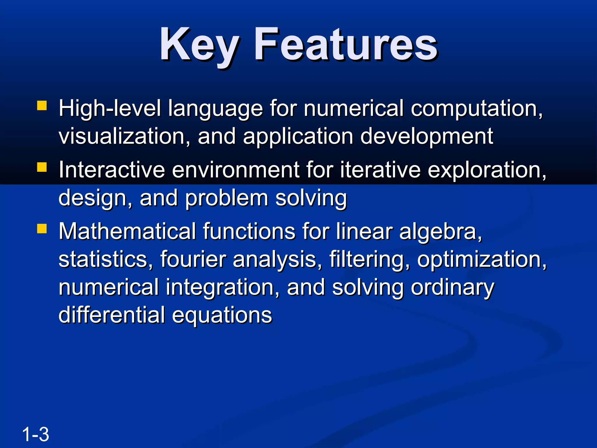
5. Key FeaturesKey Features
 High-level language for numerical computation,High-level language for numerical computation,
visualization, and application developmentvisualization, and application development
 Interactive environment for iterative exploration,Interactive environment for iterative exploration,
design, and problem solvingdesign, and problem solving
 Mathematical functions for linear algebra,Mathematical functions for linear algebra,
statistics, fourier analysis, filtering, optimization,statistics, fourier analysis, filtering, optimization,
numerical integration, and solving ordinarynumerical integration, and solving ordinary
differential equationsdifferential equations
1-3

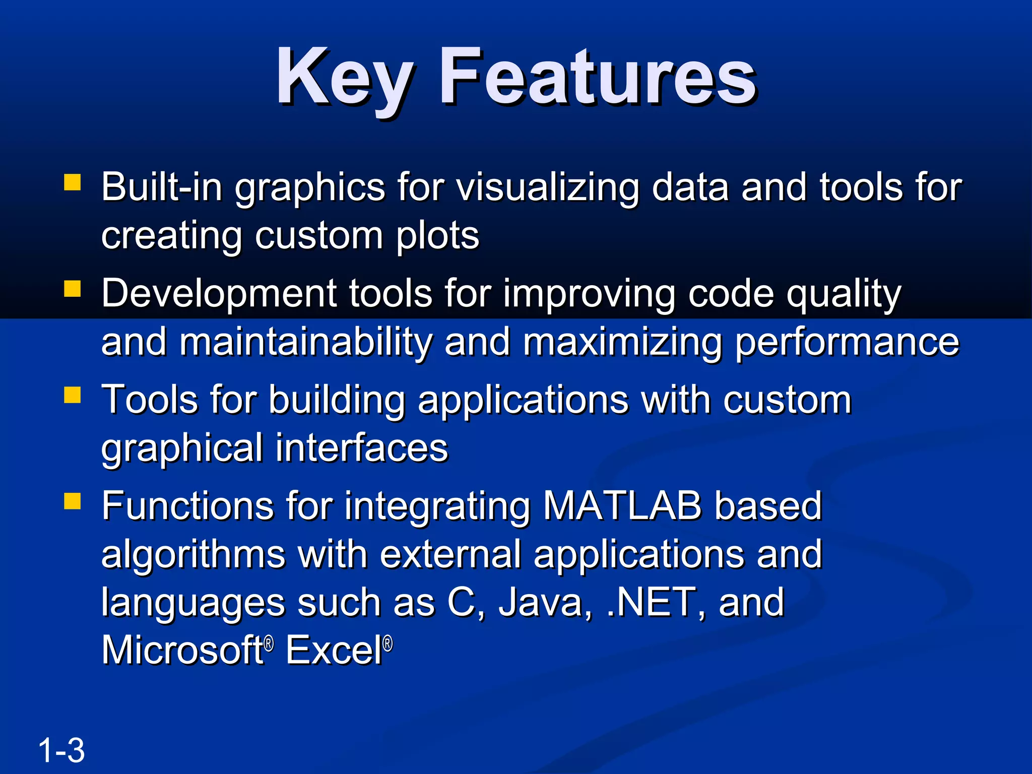
6. Key FeaturesKey Features
 Built-in graphics for visualizing data and tools forBuilt-in graphics for visualizing data and tools for
creating custom plotscreating custom plots
 Development tools for improving code qualityDevelopment tools for improving code quality
and maintainability and maximizing performanceand maintainability and maximizing performance
 Tools for building applications with customTools for building applications with custom
graphical interfacesgraphical interfaces
 Functions for integrating MATLAB basedFunctions for integrating MATLAB based
algorithms with external applications andalgorithms with external applications and
languages such as C, Java, .NET, andlanguages such as C, Java, .NET, and
MicrosoftMicrosoft®®
ExcelExcel®®
1-3

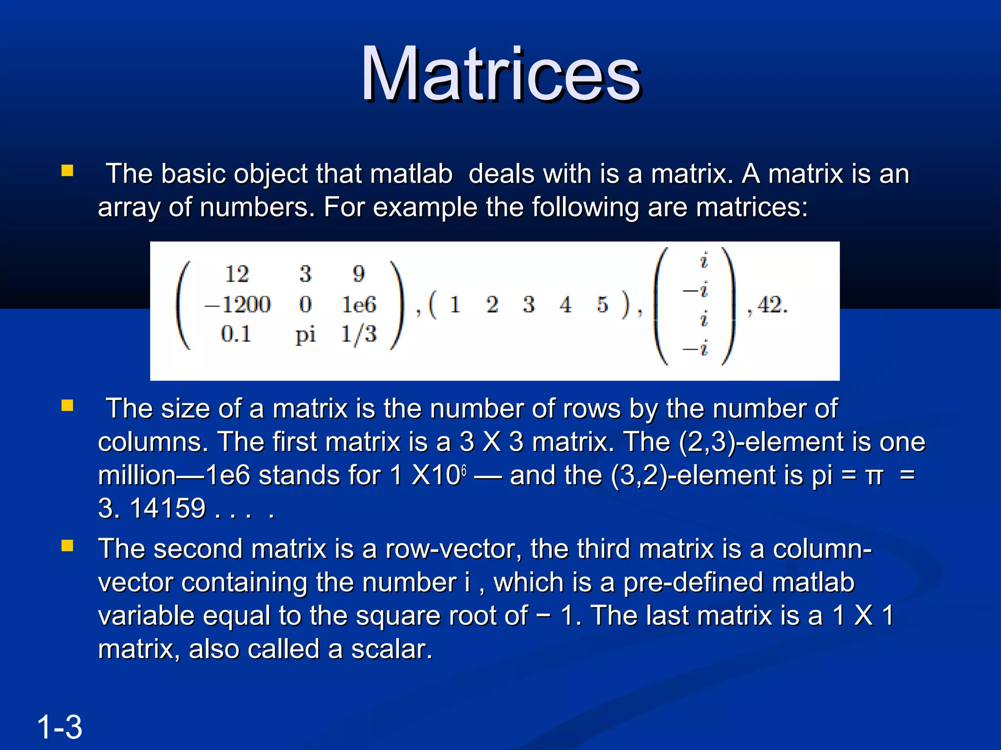
7. MatricesMatrices
 The basic object that matlab deals with is a matrix. A matrix is anThe basic object that matlab deals with is a matrix. A matrix is an
array of numbers. For example the following are matrices:array of numbers. For example the following are matrices:
 The size of a matrix is the number of rows by the number ofThe size of a matrix is the number of rows by the number of
columns. The first matrix is a 3 X 3 matrix. The (2,3)-element is onecolumns. The first matrix is a 3 X 3 matrix. The (2,3)-element is one
million—1e6 stands for 1 X10million—1e6 stands for 1 X1066
— and the (3,2)-element is pi = π =— and the (3,2)-element is pi = π =
3. 14159 . . . .3. 14159 . . . .
 The second matrix is a row-vector, the third matrix is a column-The second matrix is a row-vector, the third matrix is a column-
vector containing the number i , which is a pre-defined matlabvector containing the number i , which is a pre-defined matlab
variable equal to the square root of − 1. The last matrix is a 1 X 1variable equal to the square root of − 1. The last matrix is a 1 X 1
matrix, also called a scalar.matrix, also called a scalar.
1-3

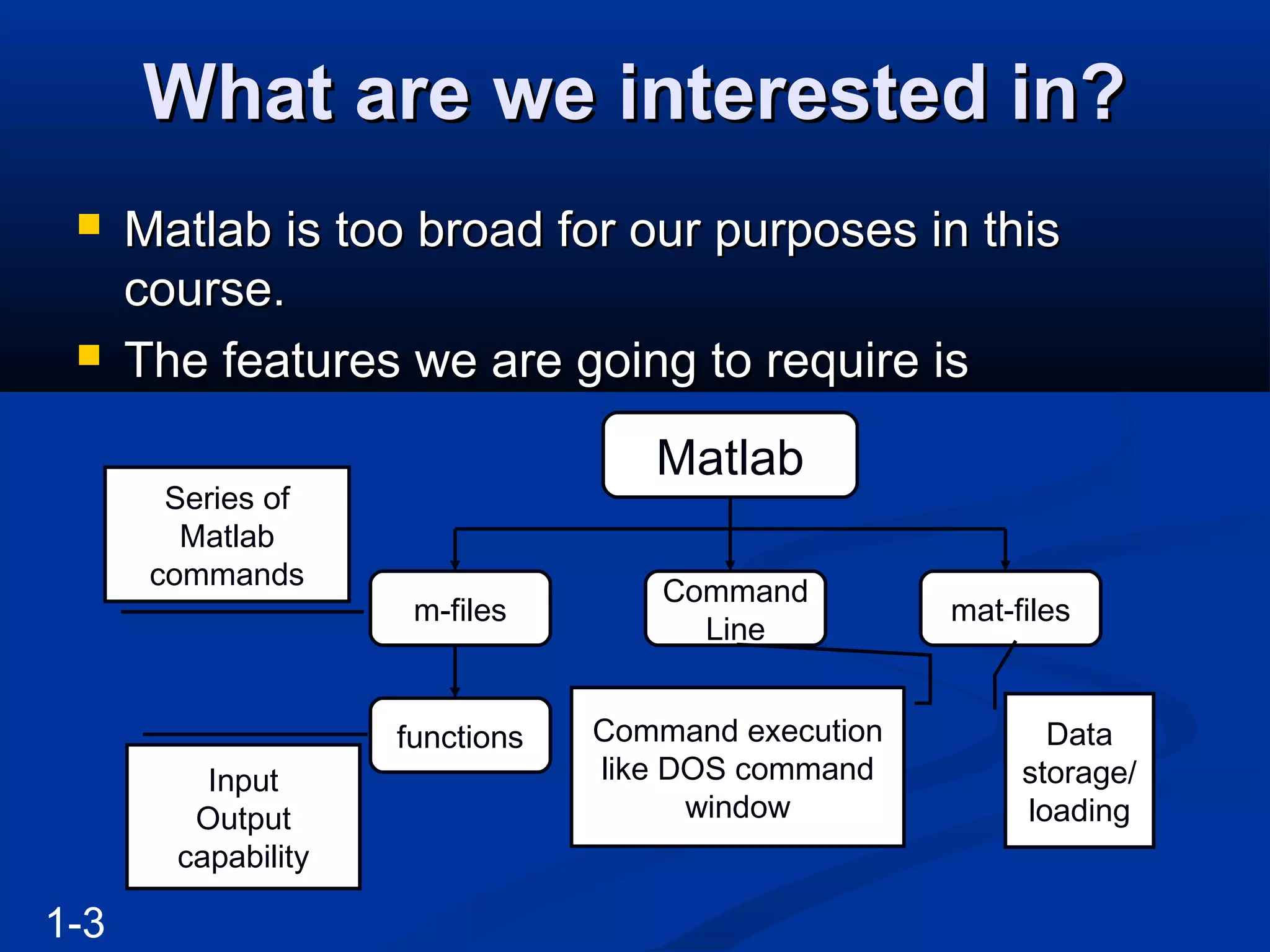
8. What are we interested in?What are we interested in?
 Matlab is too broad for our purposes in thisMatlab is too broad for our purposes in this
course.course.
 The features we are going to require isThe features we are going to require is
1-3
Matlab
Command
Line
m-files
functions
mat-files
Command execution
like DOS command
window
Series of
Matlab
commands
Input
Output
capability
Data
storage/
loading

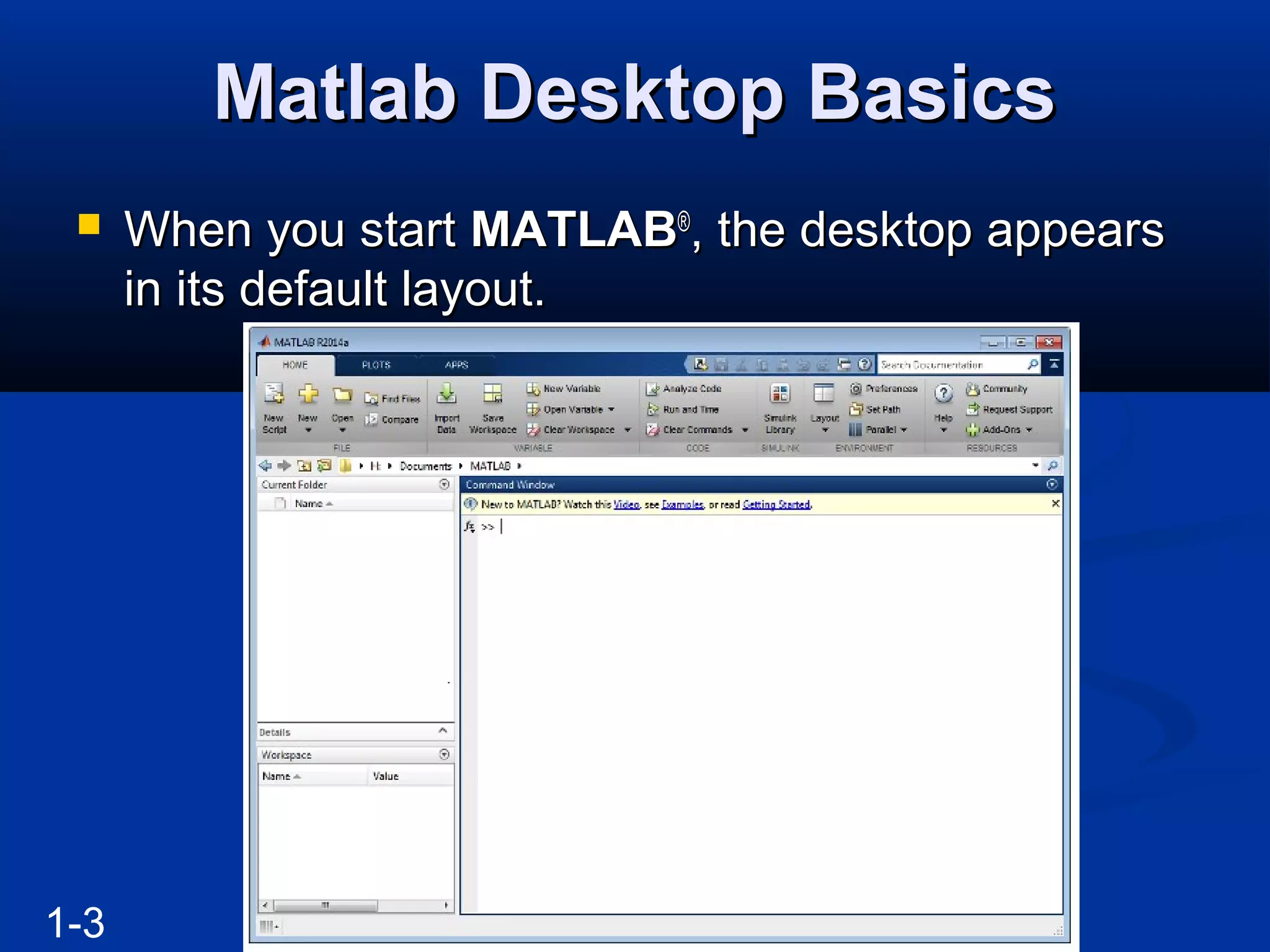
9. Matlab Desktop BasicsMatlab Desktop Basics
 When you startWhen you start MATLABMATLAB®®
, the desktop appears, the desktop appears
in its default layout.in its default layout.
1-3

10. The default MATLAB Desktop. Figure 1.1–1
1-21-2

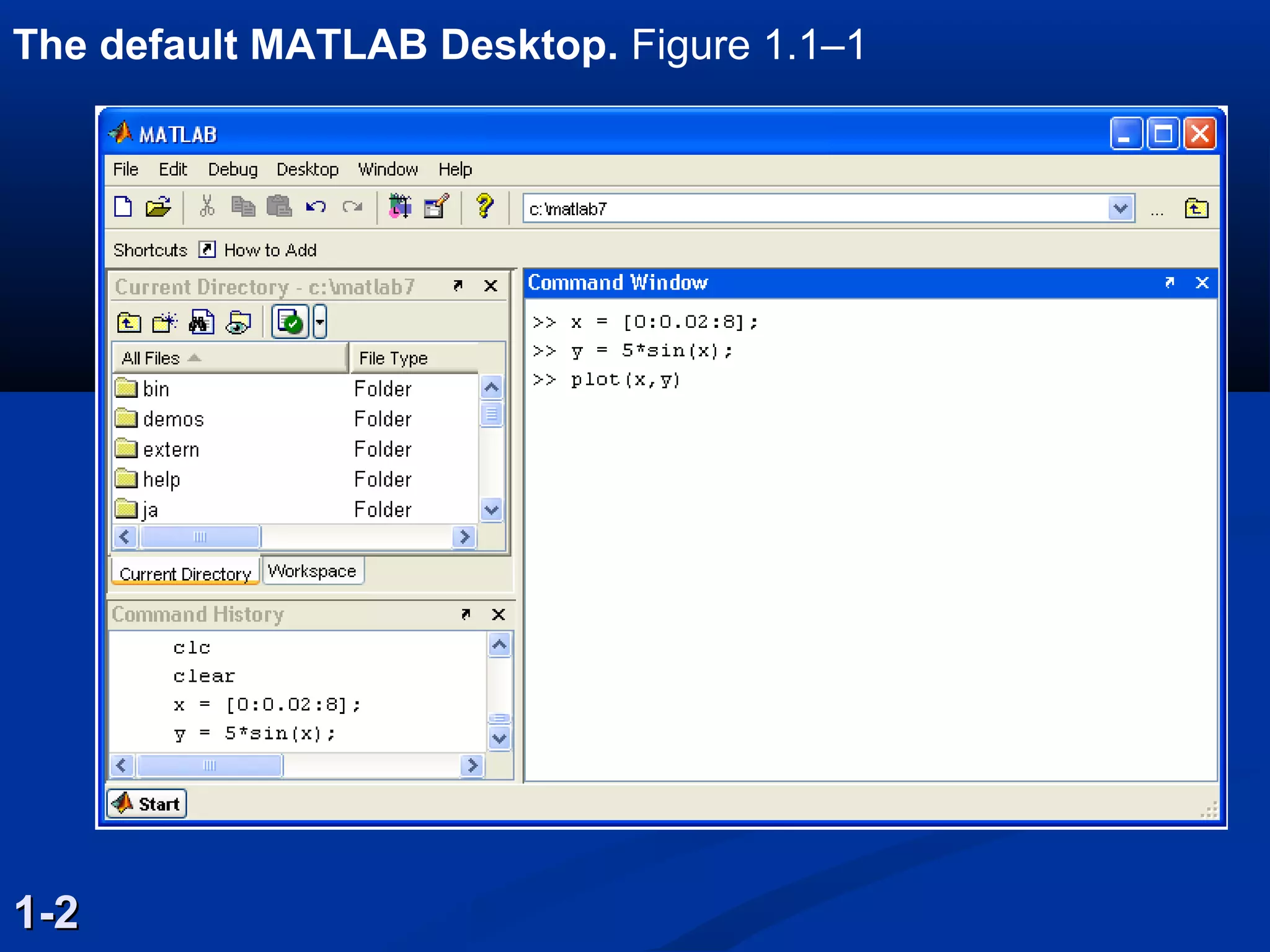
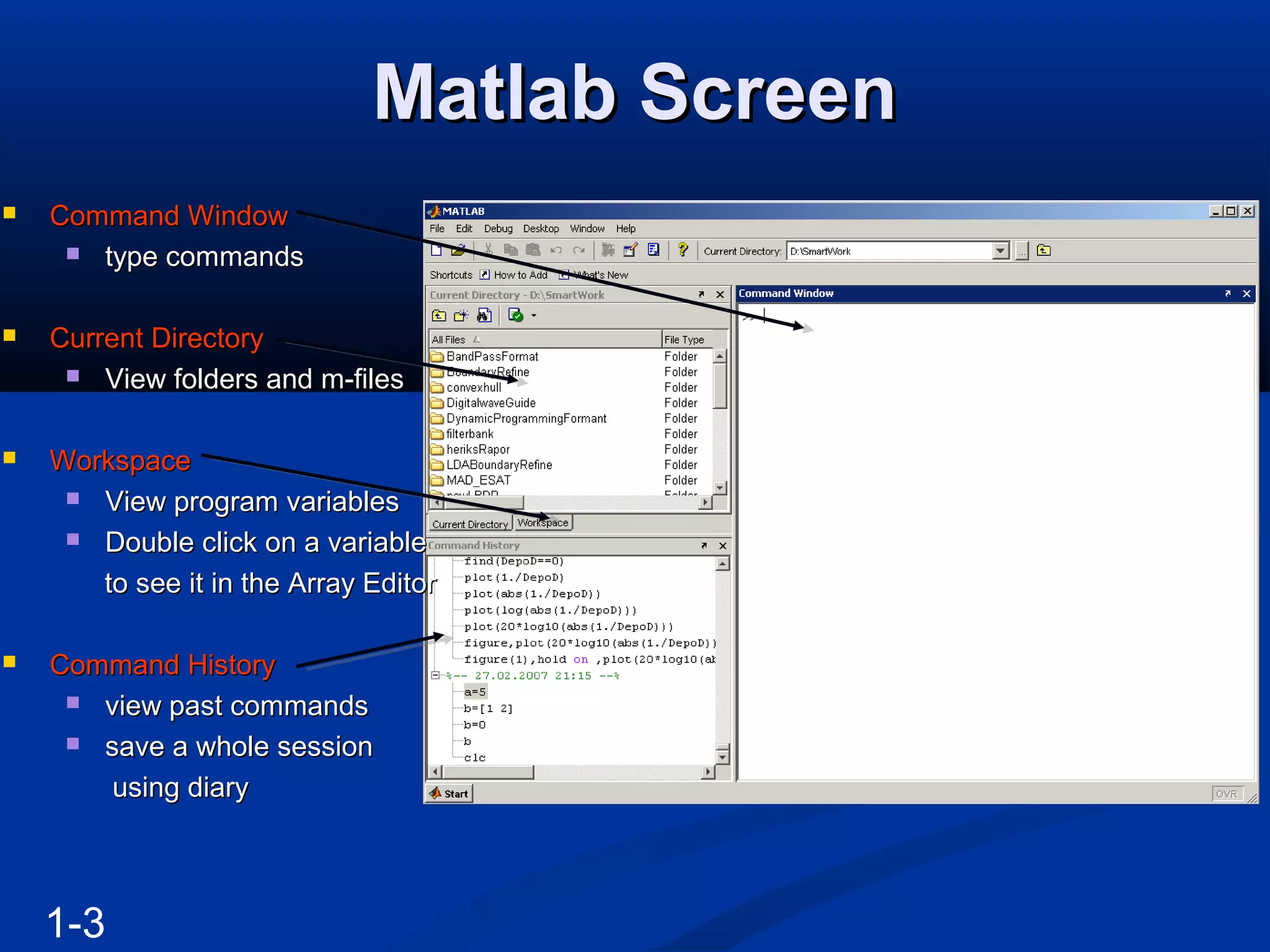
11. Matlab ScreenMatlab Screen
1-3
 Command WindowCommand Window
 type commandstype commands
 Current DirectoryCurrent Directory
 View folders and m-filesView folders and m-files
 WorkspaceWorkspace
 View program variablesView program variables
 Double click on a variableDouble click on a variable
to see it in the Array Editorto see it in the Array Editor
 Command HistoryCommand History
 view past commandsview past commands
 save a whole sessionsave a whole session
using diaryusing diary

12. Entering Commands and Expressions
 MATLAB retains your previous keystrokes.
 Use the up-arrow key to scroll back back
through the commands.
 Press the key once to see the previous entry,
and so on.
 Use the down-arrow key to scroll forward. Edit a
line using the left- and right-arrow keys the
Backspace key, and the Delete key.
 Press the Enter key to execute the command.
1-3

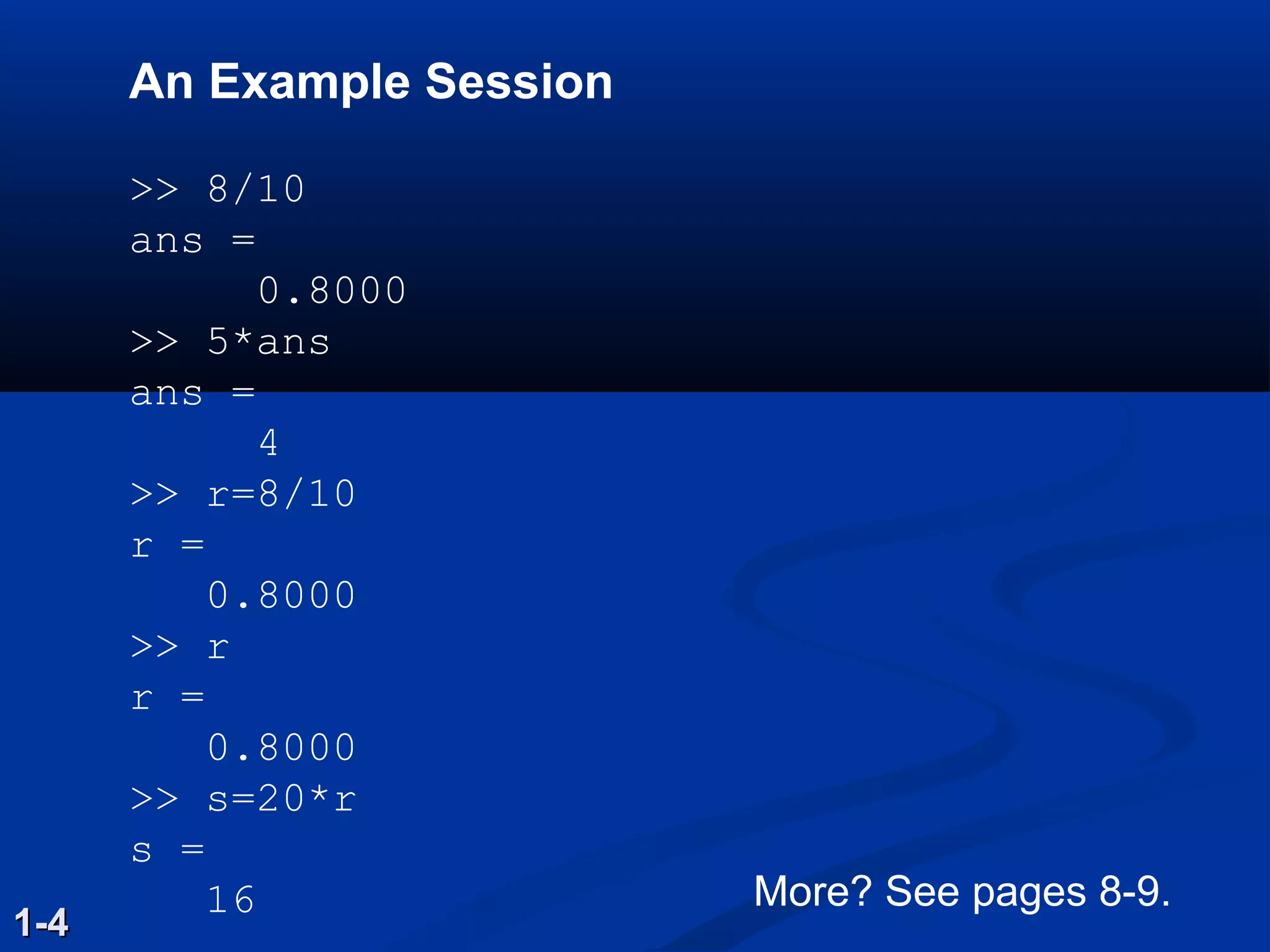
13. An Example Session
>> 8/10
ans =
0.8000
>> 5*ans
ans =
4
>> r=8/10
r =
0.8000
>> r
r =
0.8000
>> s=20*r
s =
16
1-41-4
More? See pages 8-9.

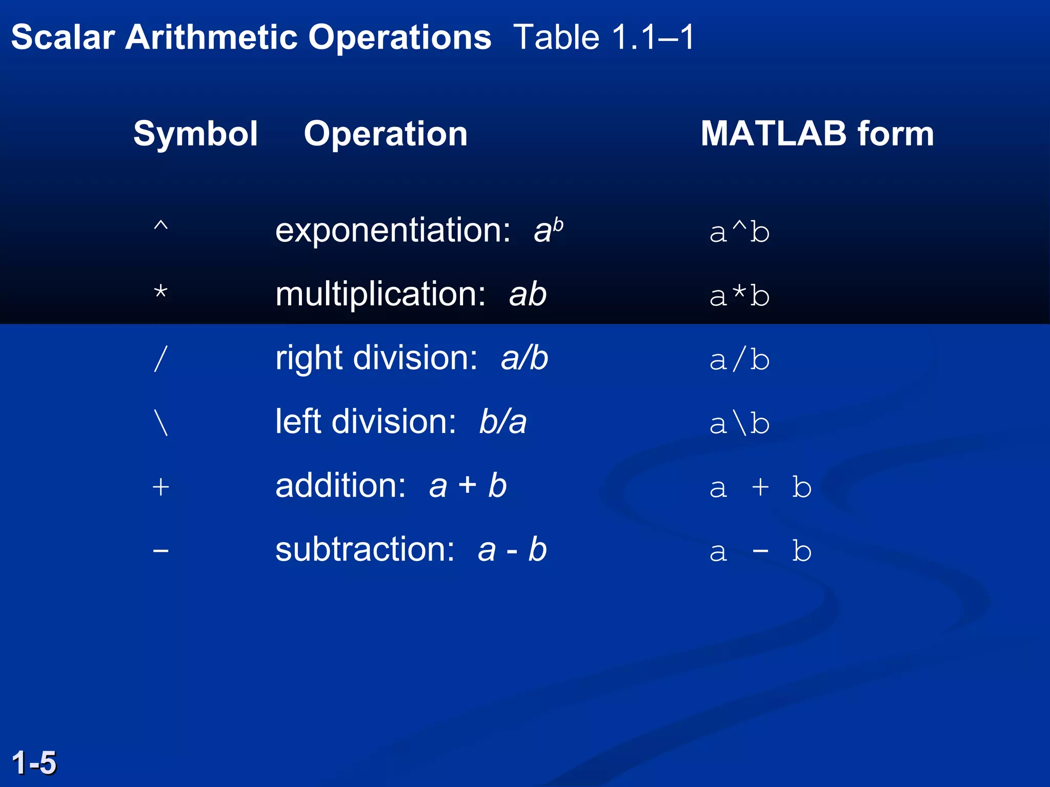
14. Scalar Arithmetic Operations Table 1.1–1
1-51-5
Symbol Operation MATLAB form
^ exponentiation: ab
a^b
* multiplication: ab a*b
/ right division: a/b a/b
left division: b/a ab
+ addition: a + b a + b
- subtraction: a - b a - b

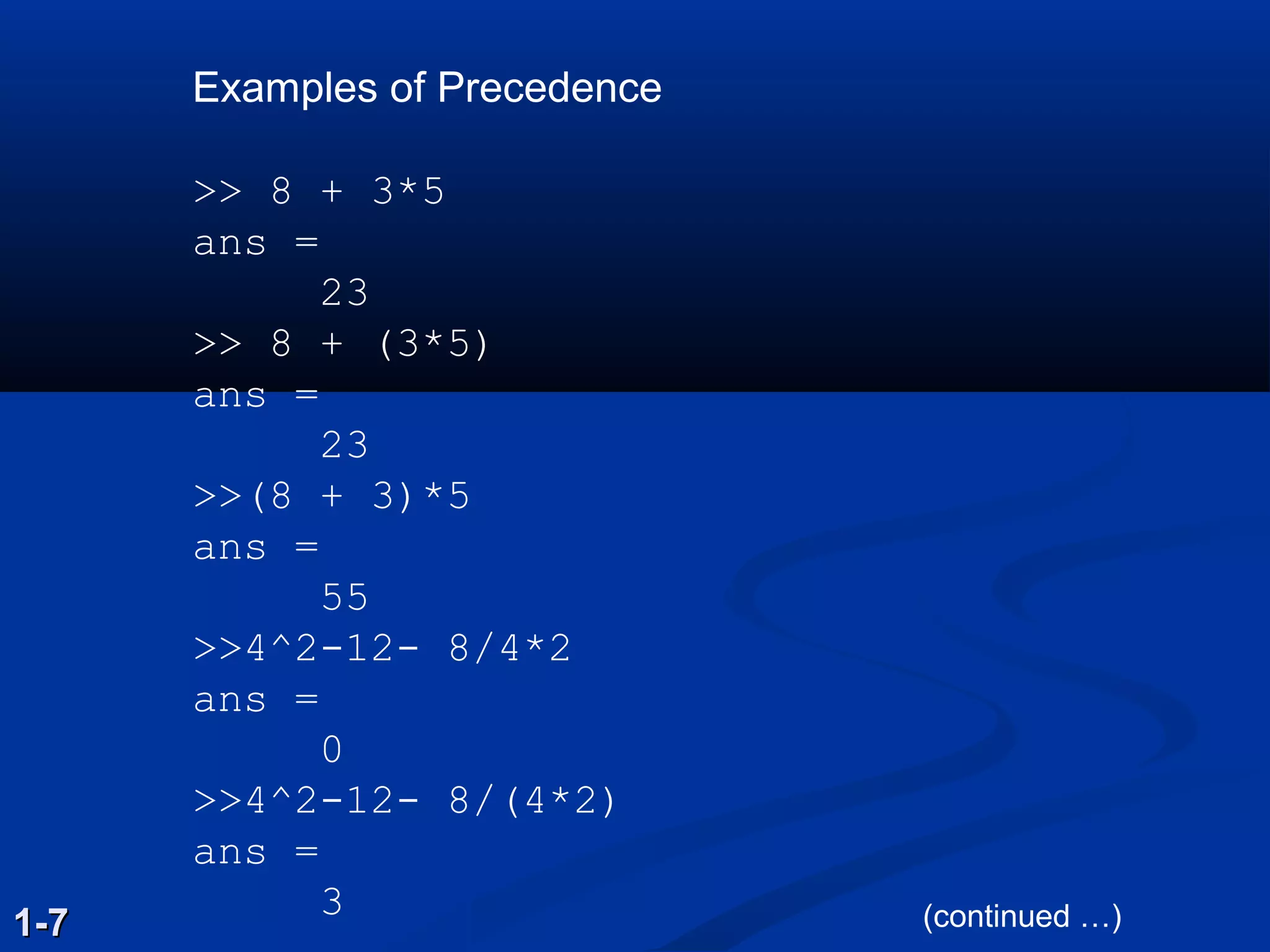
15. Examples of Precedence
>> 8 + 3*5
ans =
23
>> 8 + (3*5)
ans =
23
>>(8 + 3)*5
ans =
55
>>4^2-12- 8/4*2
ans =
0
>>4^2-12- 8/(4*2)
ans =
3
1-71-7 (continued …)

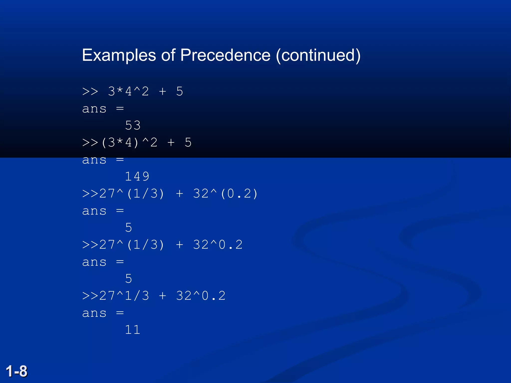
16. Examples of Precedence (continued)
>> 3*4^2 + 5
ans =
53
>>(3*4)^2 + 5
ans =
149
>>27^(1/3) + 32^(0.2)
ans =
5
>>27^(1/3) + 32^0.2
ans =
5
>>27^1/3 + 32^0.2
ans =
11
1-81-8

17. The Assignment OperatorThe Assignment Operator ==
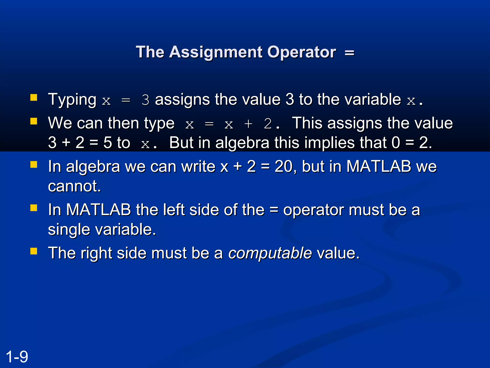
 TypingTyping x = 3x = 3 assigns the value 3 to the variableassigns the value 3 to the variable x.x.
 We can then typeWe can then type x = x + 2.x = x + 2. This assigns the valueThis assigns the value
3 + 2 = 5 to3 + 2 = 5 to x.x. But in algebra this implies that 0 = 2.But in algebra this implies that 0 = 2.
 In algebra we can write x + 2 = 20, but in MATLAB weIn algebra we can write x + 2 = 20, but in MATLAB we
cannot.cannot.
 In MATLAB the left side of the = operator must be aIn MATLAB the left side of the = operator must be a
single variable.single variable.
 The right side must be aThe right side must be a computablecomputable value.value.
1-9

18. VariablesVariables
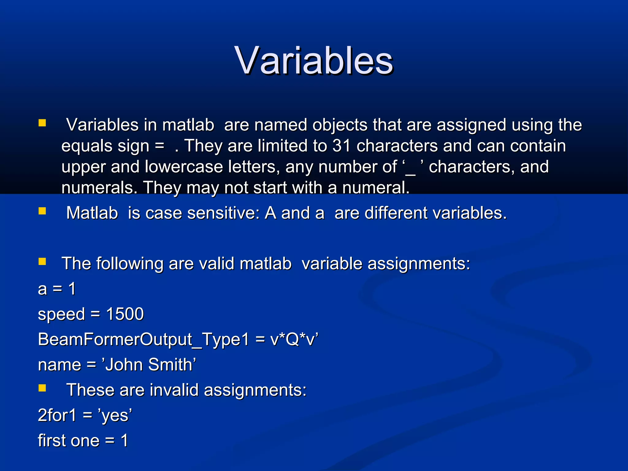
 Variables in matlab are named objects that are assigned using theVariables in matlab are named objects that are assigned using the
equals sign = . They are limited to 31 characters and can containequals sign = . They are limited to 31 characters and can contain
upper and lowercase letters, any number of ‘_ ’ characters, andupper and lowercase letters, any number of ‘_ ’ characters, and
numerals. They may not start with a numeral.numerals. They may not start with a numeral.
 Matlab is case sensitive: A and a are different variables.Matlab is case sensitive: A and a are different variables.
 The following are valid matlab variable assignments:The following are valid matlab variable assignments:
a = 1a = 1
speed = 1500speed = 1500
BeamFormerOutput_Type1 = v*Q*vBeamFormerOutput_Type1 = v*Q*v’’
name =name = ’’John SmithJohn Smith’’
 These are invalid assignments:These are invalid assignments:
2for1 =2for1 = ’’yesyes’’
first one = 1first one = 1

19. Try typing the following:Try typing the following:
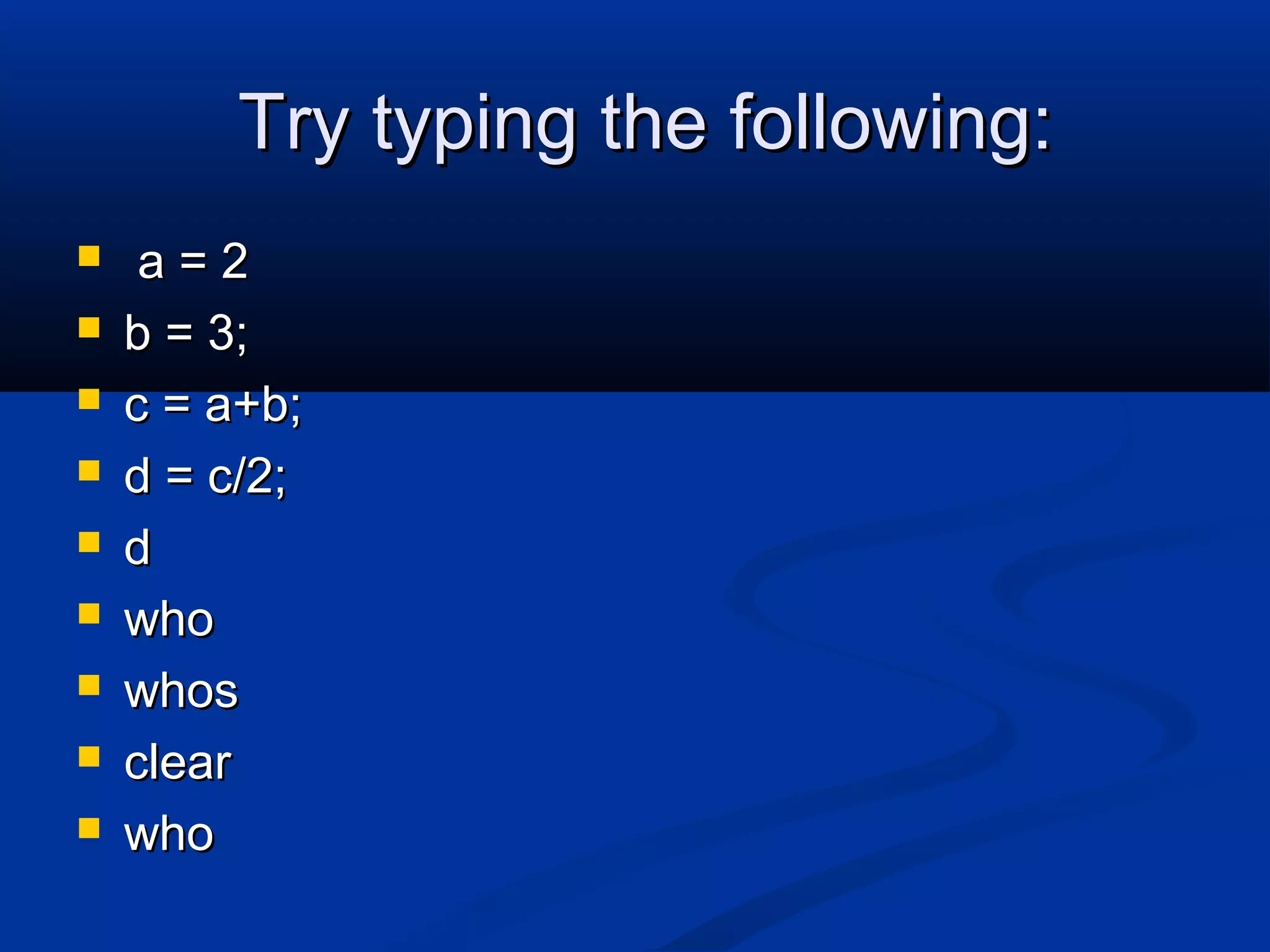
 a = 2a = 2
 b = 3;b = 3;
 c = a+b;c = a+b;
 d = c/2;d = c/2;
 dd
 whowho
 whoswhos
 clearclear
 whowho

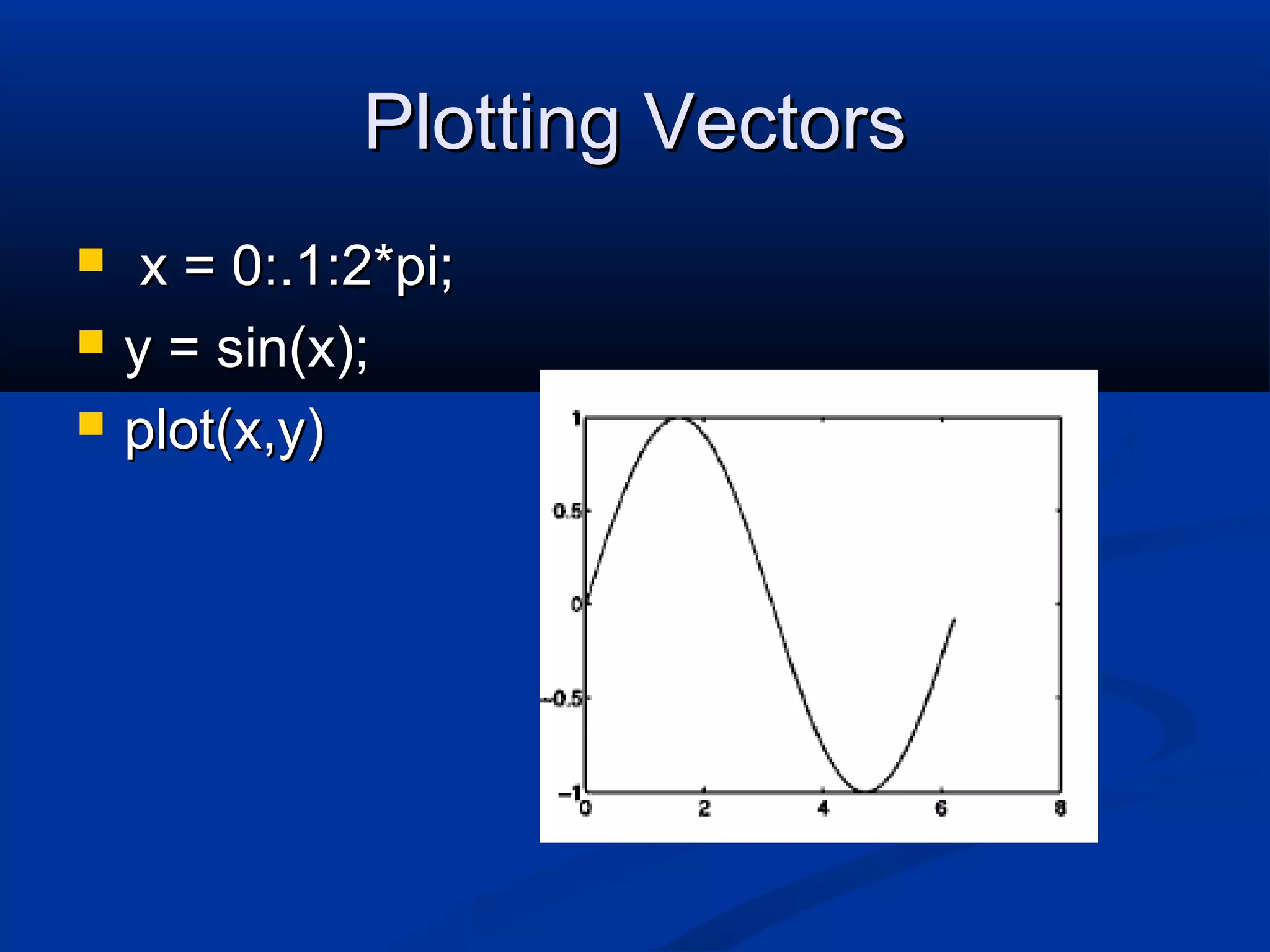
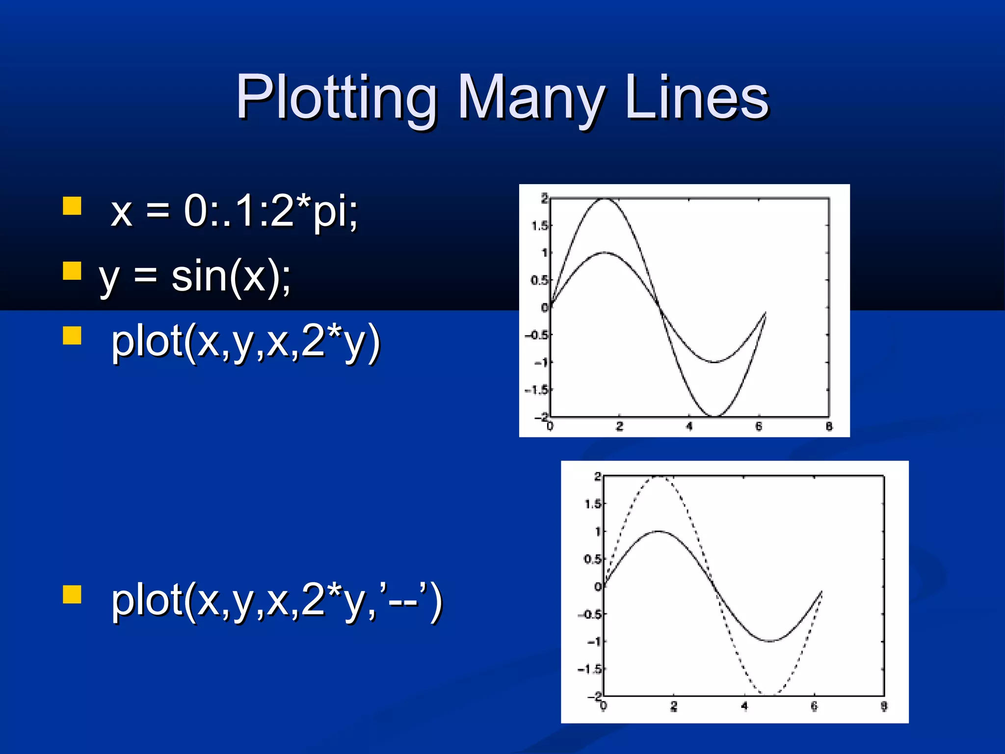
20. The Colon OperatorThe Colon Operator
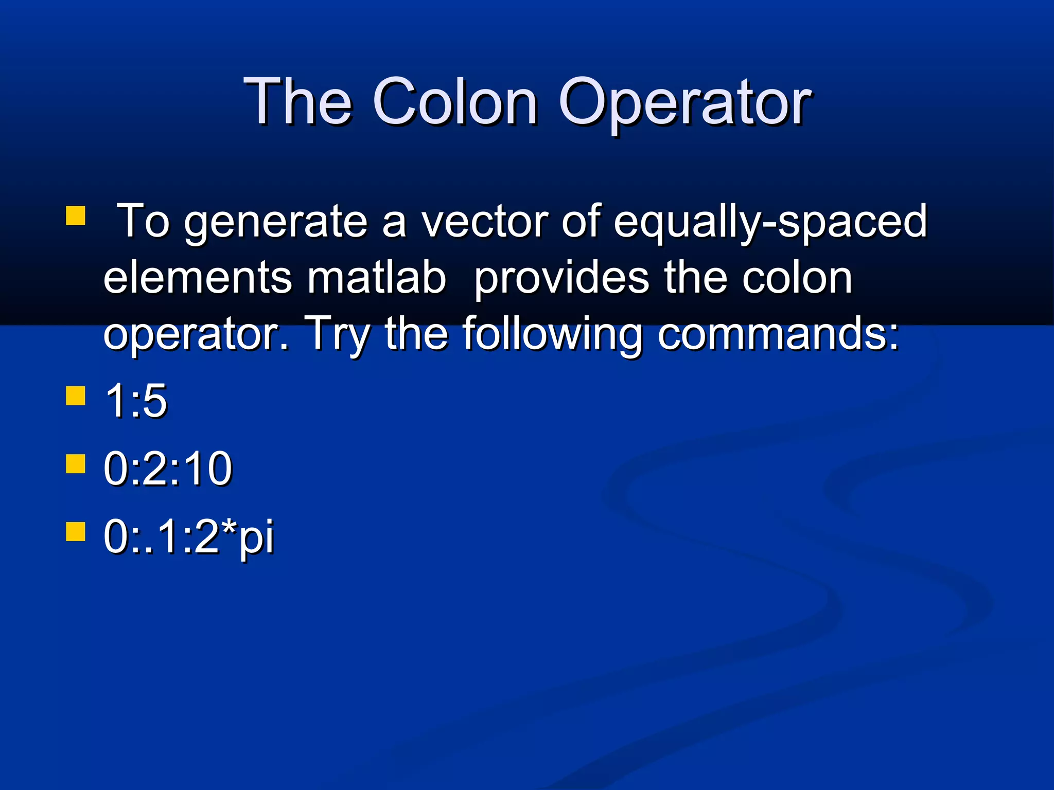
 To generate a vector of equally-spacedTo generate a vector of equally-spaced
elements matlab provides the colonelements matlab provides the colon
operator. Try the following commands:operator. Try the following commands:
 1:51:5
 0:2:100:2:10
 0:.1:2*pi0:.1:2*pi

21. Plotting VectorsPlotting Vectors
 x = 0:.1:2*pi;x = 0:.1:2*pi;
 y = sin(x);y = sin(x);
 plot(x,y)plot(x,y)

22. Plotting Many LinesPlotting Many Lines
 x = 0:.1:2*pi;x = 0:.1:2*pi;
 y = sin(x);y = sin(x);
 plot(x,y,x,2*y)plot(x,y,x,2*y)
 plot(x,y,x,2*y,plot(x,y,x,2*y,’’----’’))

23. Adding PlotsAdding Plots
 plot(x,y)plot(x,y)
 hold onhold on
 plot(5*x,5*y)plot(5*x,5*y)

24. Plotting MatricesPlotting Matrices
 one line per columnone line per column
 >> q = [1 1 1;2 3 4;3 5 7;4 7 10]>> q = [1 1 1;2 3 4;3 5 7;4 7 10]
 q =q =
11 11 11
22 33 44
33 55 77
44 77 1010
 >> plot(q)>> plot(q)
 >> grid>> grid

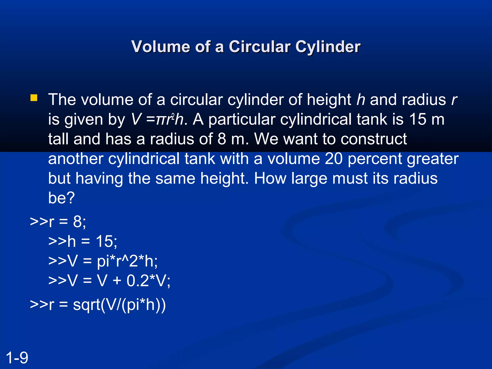
25. Volume of a Circular CylinderVolume of a Circular Cylinder
 The volume of a circular cylinder of height h and radius r
is given by V =πr2
h. A particular cylindrical tank is 15 m
tall and has a radius of 8 m. We want to construct
another cylindrical tank with a volume 20 percent greater
but having the same height. How large must its radius
be?
>>r = 8;
>>h = 15;
>>V = pi*r^2*h;
>>V = V + 0.2*V;
>>r = sqrt(V/(pi*h))
1-9

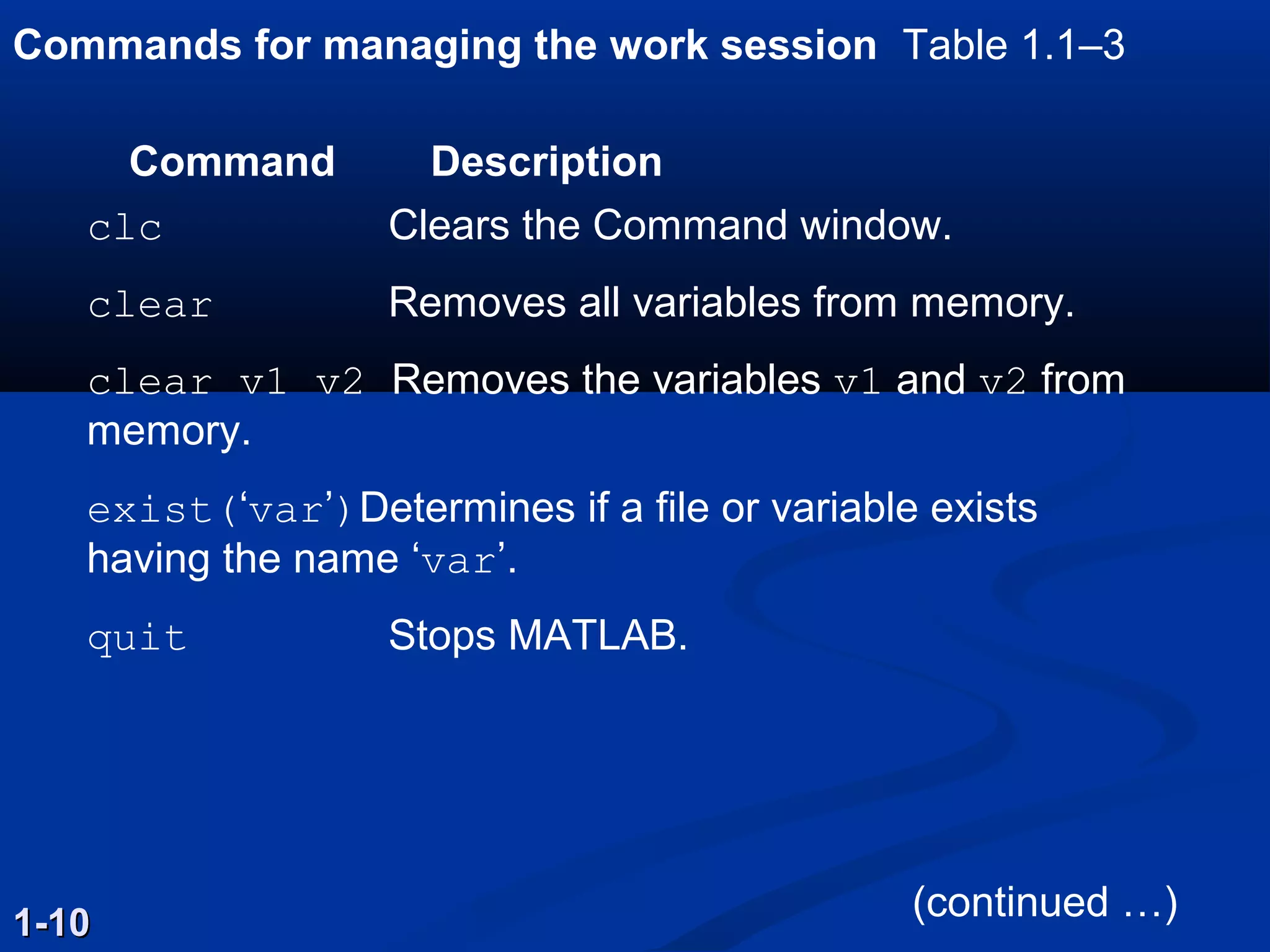
26. Commands for managing the work session Table 1.1–3
1-101-10
Command Description
clc Clears the Command window.
clear Removes all variables from memory.
clear v1 v2 Removes the variables v1 and v2 from
memory.
exist(‘var’)Determines if a file or variable exists
having the name ‘var’.
quit Stops MATLAB.
(continued …)

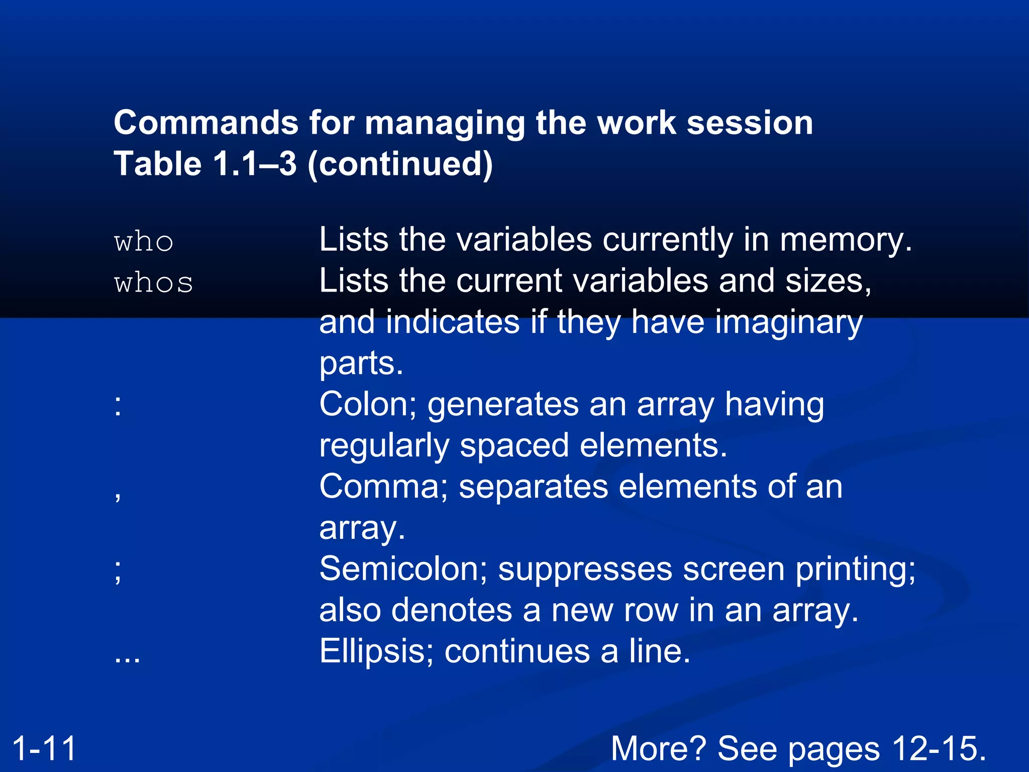
27. Commands for managing the work session
Table 1.1–3 (continued)
who Lists the variables currently in memory.
whos Lists the current variables and sizes,
and indicates if they have imaginary
parts.
: Colon; generates an array having
regularly spaced elements.
, Comma; separates elements of an
array.
; Semicolon; suppresses screen printing;
also denotes a new row in an array.
... Ellipsis; continues a line.
1-11 More? See pages 12-15.

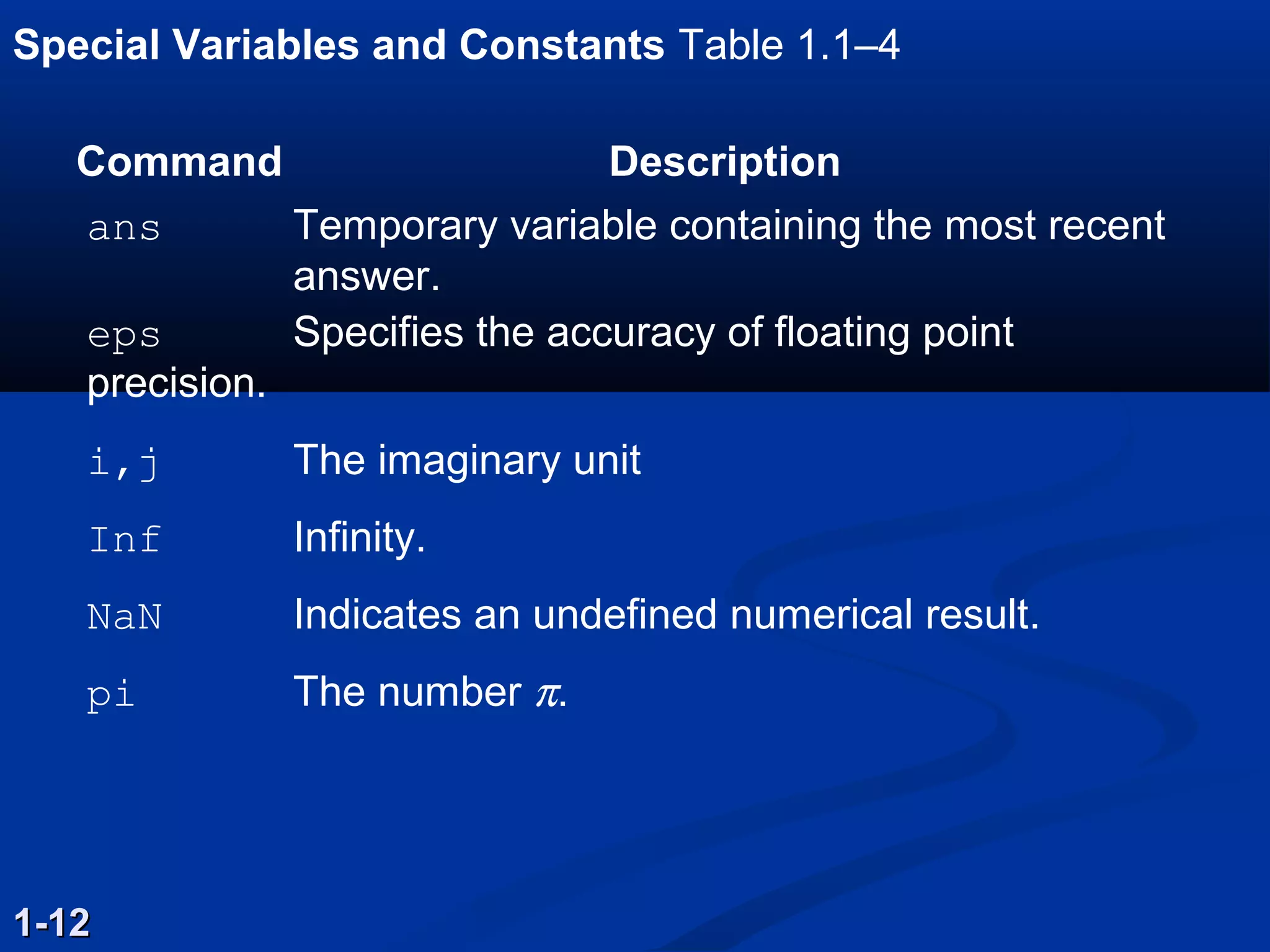
28. Special Variables and Constants Table 1.1–4
1-121-12
Command Description
ans Temporary variable containing the most recent
answer.
eps Specifies the accuracy of floating point
precision.
i,j The imaginary unit
Inf Infinity.
NaN Indicates an undefined numerical result.
pi The number π.

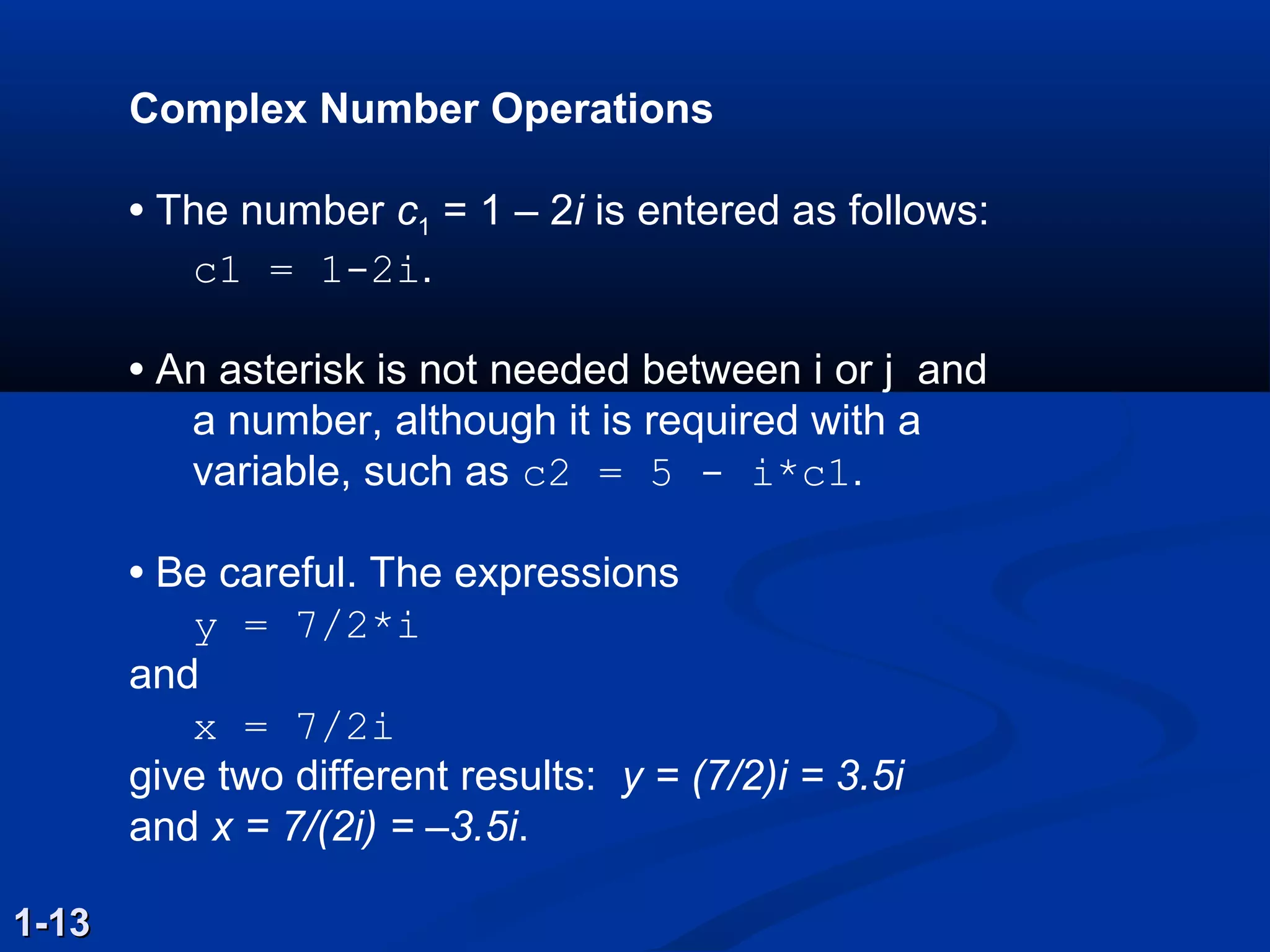
29. Complex Number Operations
• The number c1 = 1 – 2i is entered as follows:
c1 = 1­2i.
• An asterisk is not needed between i or j and
a number, although it is required with a
variable, such as c2 = 5 ­ i*c1.
• Be careful. The expressions
y = 7/2*i
and
x = 7/2i
give two different results: y = (7/2)i = 3.5i
and x = 7/(2i) = –3.5i.
1-131-13

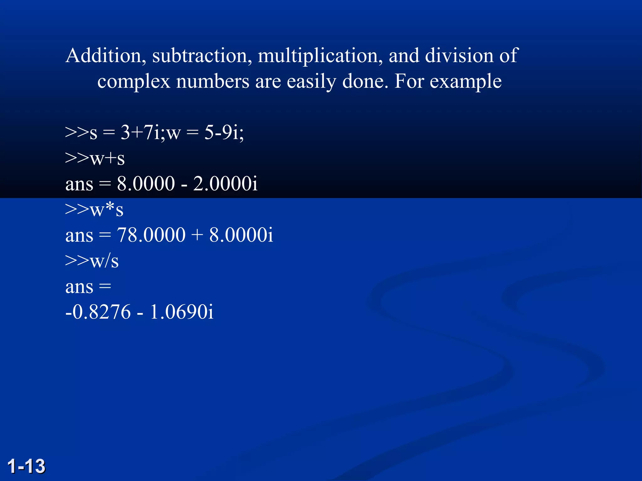
30. Addition, subtraction, multiplication, and division of
complex numbers are easily done. For example
>>s = 3+7i;w = 5-9i;
>>w+s
ans = 8.0000 - 2.0000i
>>w*s
ans = 78.0000 + 8.0000i
>>w/s
ans =
-0.8276 - 1.0690i
1-131-13

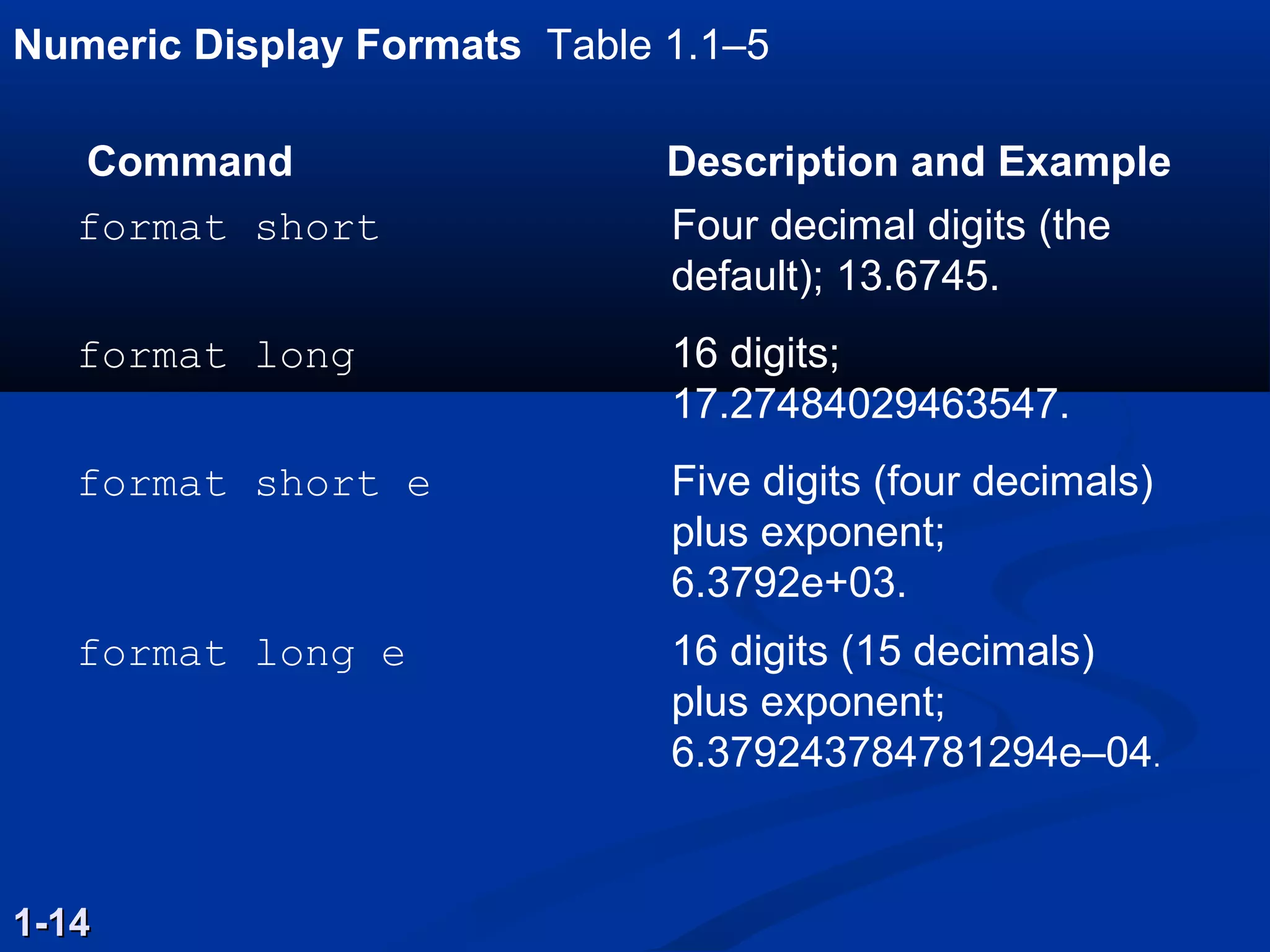
31. Numeric Display Formats Table 1.1–5
1-141-14
Command Description and Example
format short Four decimal digits (the
default); 13.6745.
format long 16 digits;
17.27484029463547.
format short e Five digits (four decimals)
plus exponent;
6.3792e+03.
format long e 16 digits (15 decimals)
plus exponent;
6.379243784781294e–04.

32. Arrays
The basic building blocks in MATLAB
• The numbers 0, 0.1, 0.2, …, 10 can be assigned to the
variable u by typing u = [0:0.1:10].
• To compute w = 5 sin u for u = 0, 0.1, 0.2, …, 10, the
session is;
>>u = [0:0.1:10];
>>w = 5*sin(u);
• The single line, w = 5*sin(u), computed the formula
w = 5 sin u 101 times.
1-151-15

33. Array Index
>>u(7)
ans =
0.6000
>>w(7)
ans =
2.8232
• Use the length function to determine
how many values are in an array.
>>m = length(w)
m =
101
1-161-16

34. Polynomial Roots
To find the roots of x3
– 7x2
+ 40x – 34 = 0, the session
is
>>a = [1,­7,40,­34];
>>roots(a)
ans =
3.0000 + 5.000i
3.0000 ­ 5.000i
1.0000
The roots are x = 1 and x = 3 ± 5i.
1-171-17

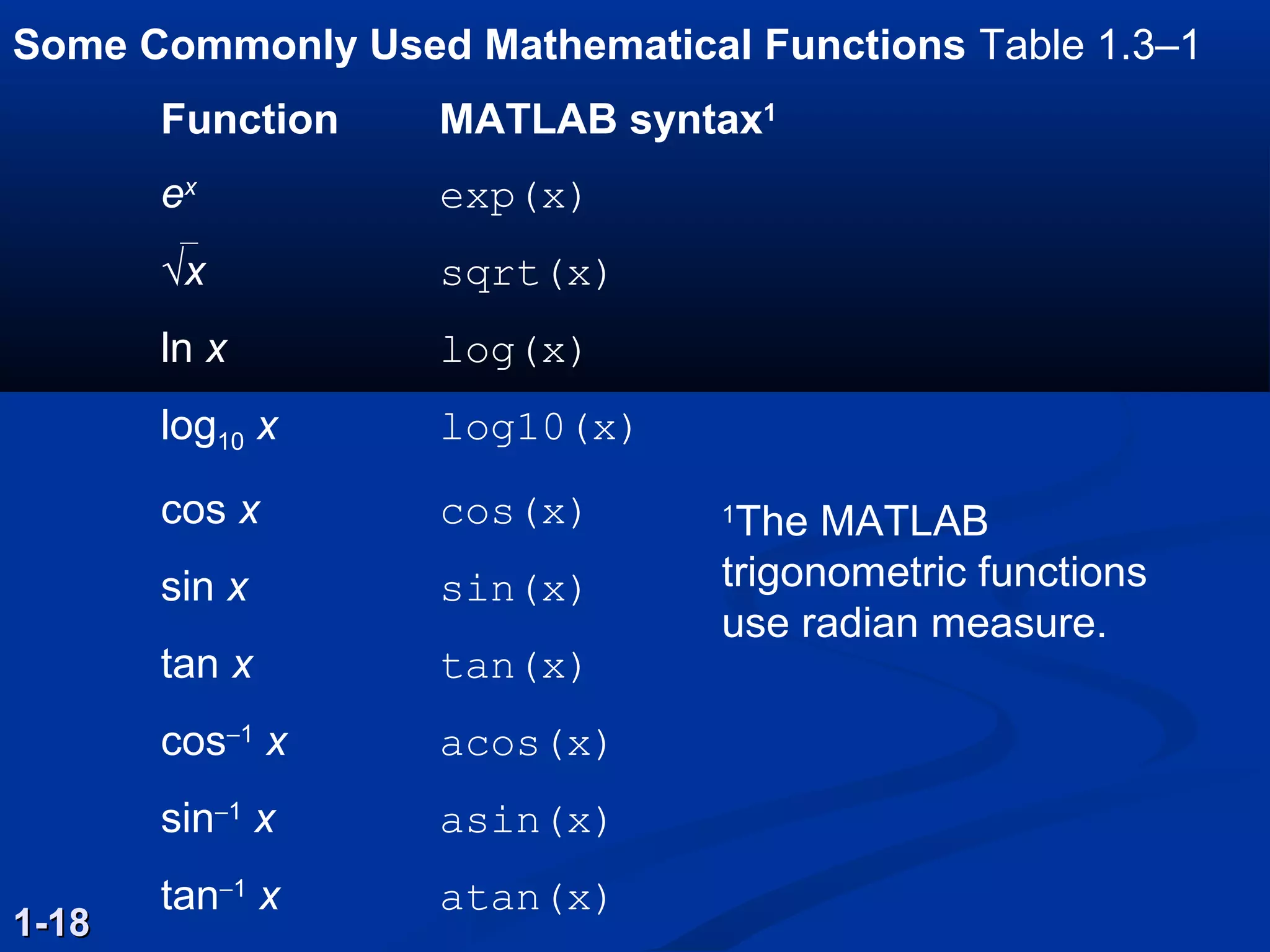
35. Some Commonly Used Mathematical Functions Table 1.3–1
1-181-18
Function MATLAB syntax1
ex
exp(x)
√x sqrt(x)
ln x log(x)
log10 x log10(x)
cos x cos(x)
sin x sin(x)
tan x tan(x)
cos−1
x acos(x)
sin−1
x asin(x)
tan−1
x atan(x)
1
The MATLAB
trigonometric functions
use radian measure.

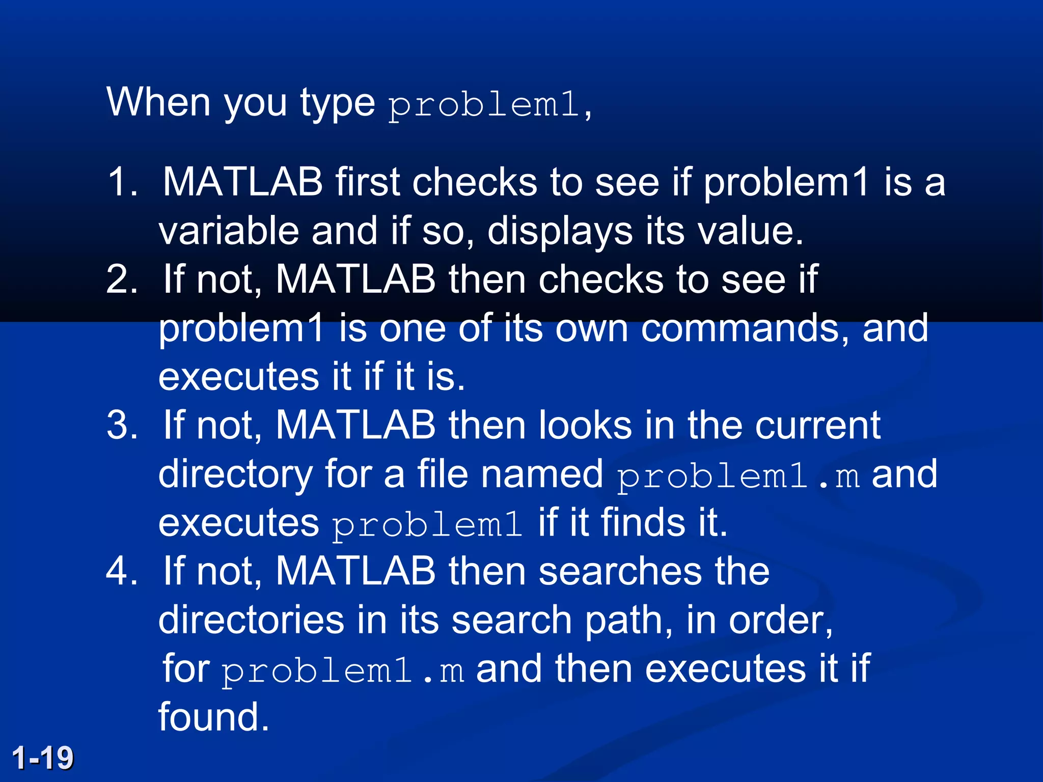
36. When you type problem1,
1. MATLAB first checks to see if problem1 is a
variable and if so, displays its value.
2. If not, MATLAB then checks to see if
problem1 is one of its own commands, and
executes it if it is.
3. If not, MATLAB then looks in the current
directory for a file named problem1.m and
executes problem1 if it finds it.
4. If not, MATLAB then searches the
directories in its search path, in order,
for problem1.m and then executes it if
found.
1-191-19

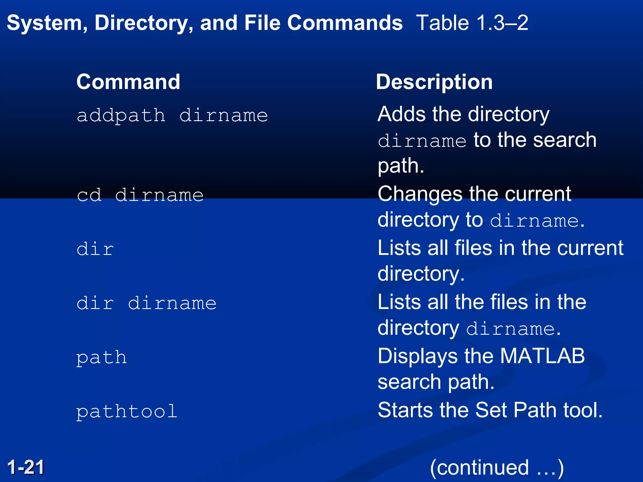
37. System, Directory, and File Commands Table 1.3–2
1-211-21
Command Description
addpath dirname Adds the directory
dirname to the search
path.
cd dirname Changes the current
directory to dirname.
dir Lists all files in the current
directory.
dir dirname Lists all the files in the
directory dirname.
path Displays the MATLAB
search path.
pathtool Starts the Set Path tool.
(continued …)

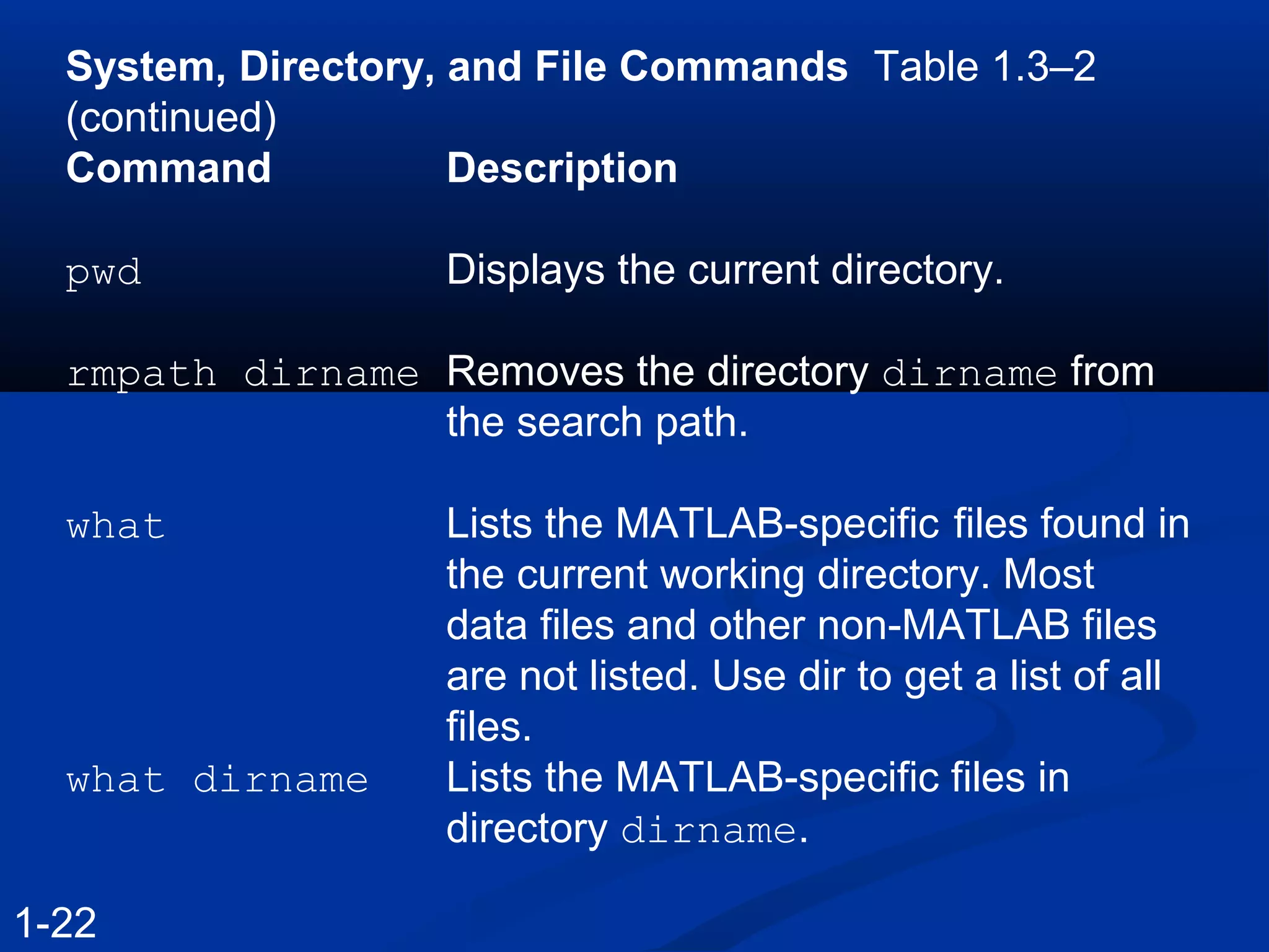
38. System, Directory, and File Commands Table 1.3–2
(continued)
Command Description
pwd Displays the current directory.
rmpath dirname Removes the directory dirname from
the search path.
what Lists the MATLAB-specific files found in
the current working directory. Most
data files and other non-MATLAB files
are not listed. Use dir to get a list of all
files.
what dirname Lists the MATLAB-specific files in
directory dirname.
1-22

39. A graphics window showing a plot. Figure 1.3–1
1-231-23

40. Some MATLAB plotting commands Table 1.3–3
1-241-24
Command Description
[x,y] = ginput(n) Enables the mouse to get n points
from a plot, and returns the x and y
coordinates in the vectors x and y,
which have a length n.
grid Puts grid lines on the plot.
gtext(’text’) Enables placement of text with the
mouse.
(continued …)

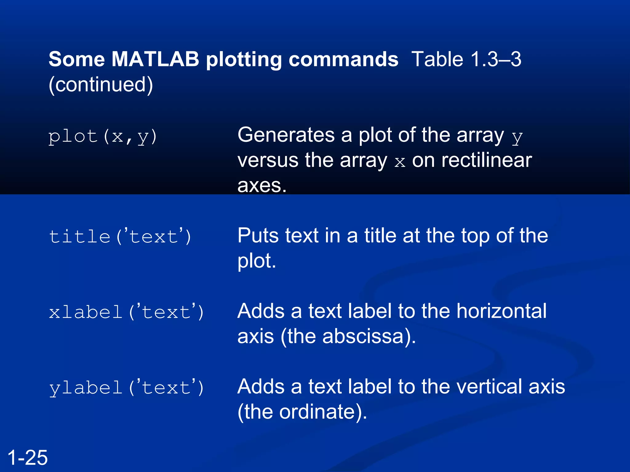
41. Some MATLAB plotting commands Table 1.3–3
(continued)
plot(x,y) Generates a plot of the array y
versus the array x on rectilinear
axes.
title(’text’) Puts text in a title at the top of the
plot.
xlabel(’text’) Adds a text label to the horizontal
axis (the abscissa).
ylabel(’text’) Adds a text label to the vertical axis
(the ordinate).
1-25

42. >> x=[0:0.01:1.5];
>> y=4*sqrt(6*x+1);
>> z=5*exp(0.3*x)-2*x;
>>plot(x,y,x,z,'--'),xlabel('meters’),…
ylabel('newtons'),gtext('y'),gtext('z')

43. Solution of Linear Algebraic Equations
6x + 12y + 4z = 70
7x – 2y + 3z = 5
2x + 8y – 9z = 64
>>A = [6,12,4;7,-2,3;2,8,-9];
>>B = [70;5;64];
>>Solution = AB
Solution =
3
5
-2
The solution is x = 3, y = 5, and z = –2.
1-261-26

44. You can perform operations in MATLAB in two
ways:
1. In the interactive mode, in which all
commands are entered directly in the
Command window, or
2. By running a MATLAB program stored in
script file.
This type of file contains MATLAB
commands, so running it is equivalent to
typing all the commands—one at a time—
at the Command window prompt.
You can run the file by typing its name at
the Command window prompt.
1-271-27

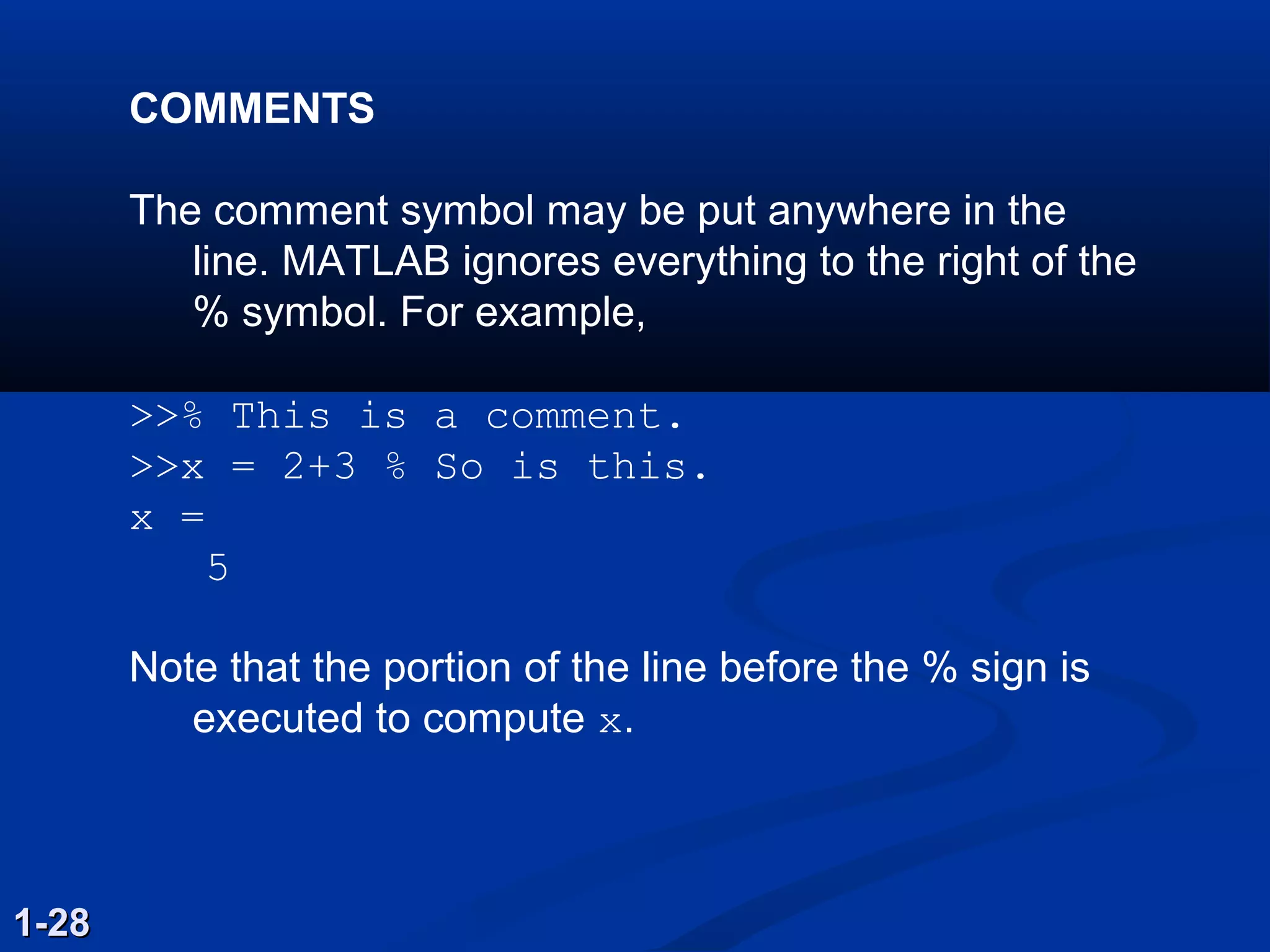
45. COMMENTS
The comment symbol may be put anywhere in the
line. MATLAB ignores everything to the right of the
% symbol. For example,
>>% This is a comment.
>>x = 2+3 % So is this.
x =
5
Note that the portion of the line before the % sign is
executed to compute x.
1-281-28

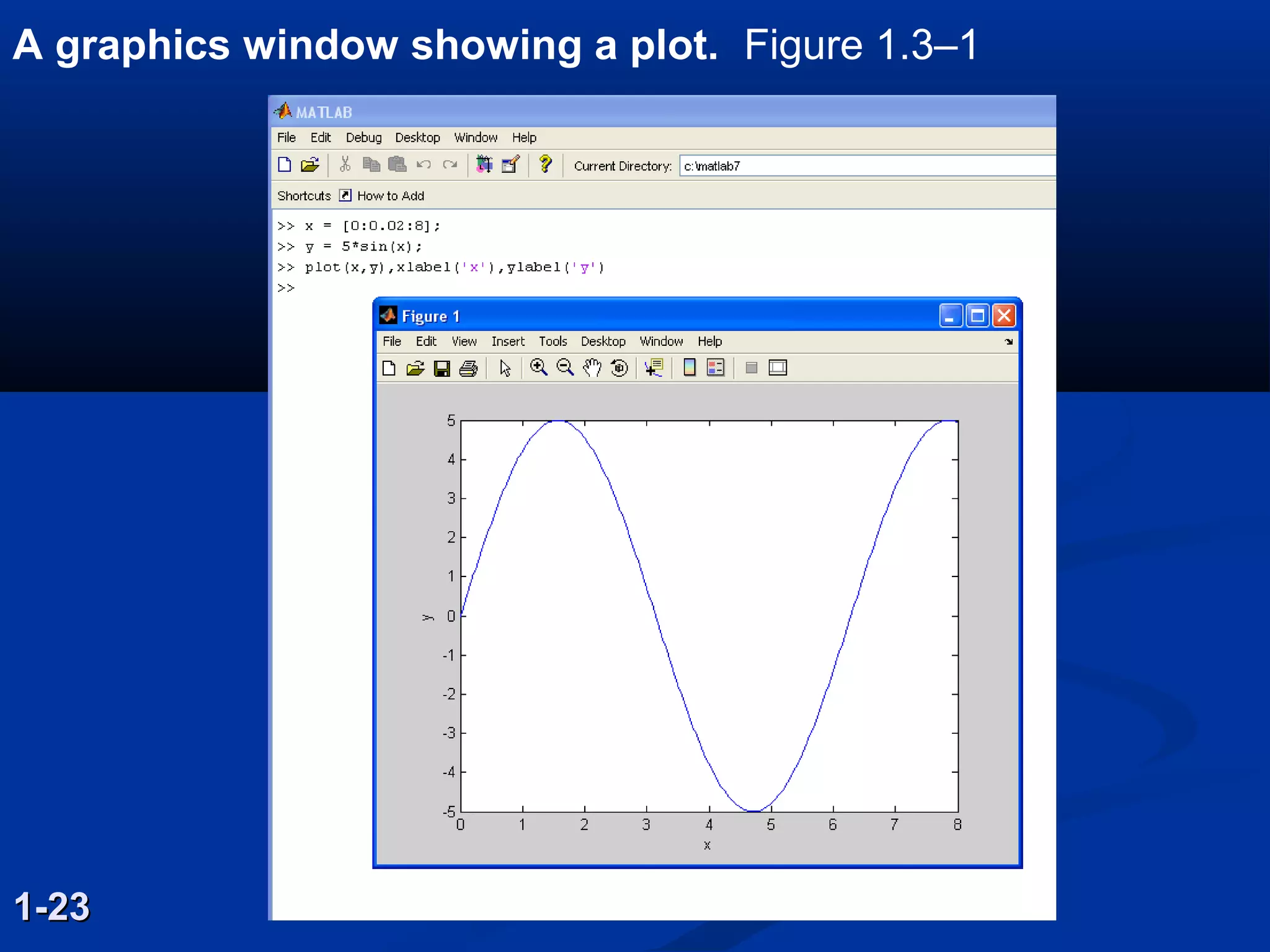
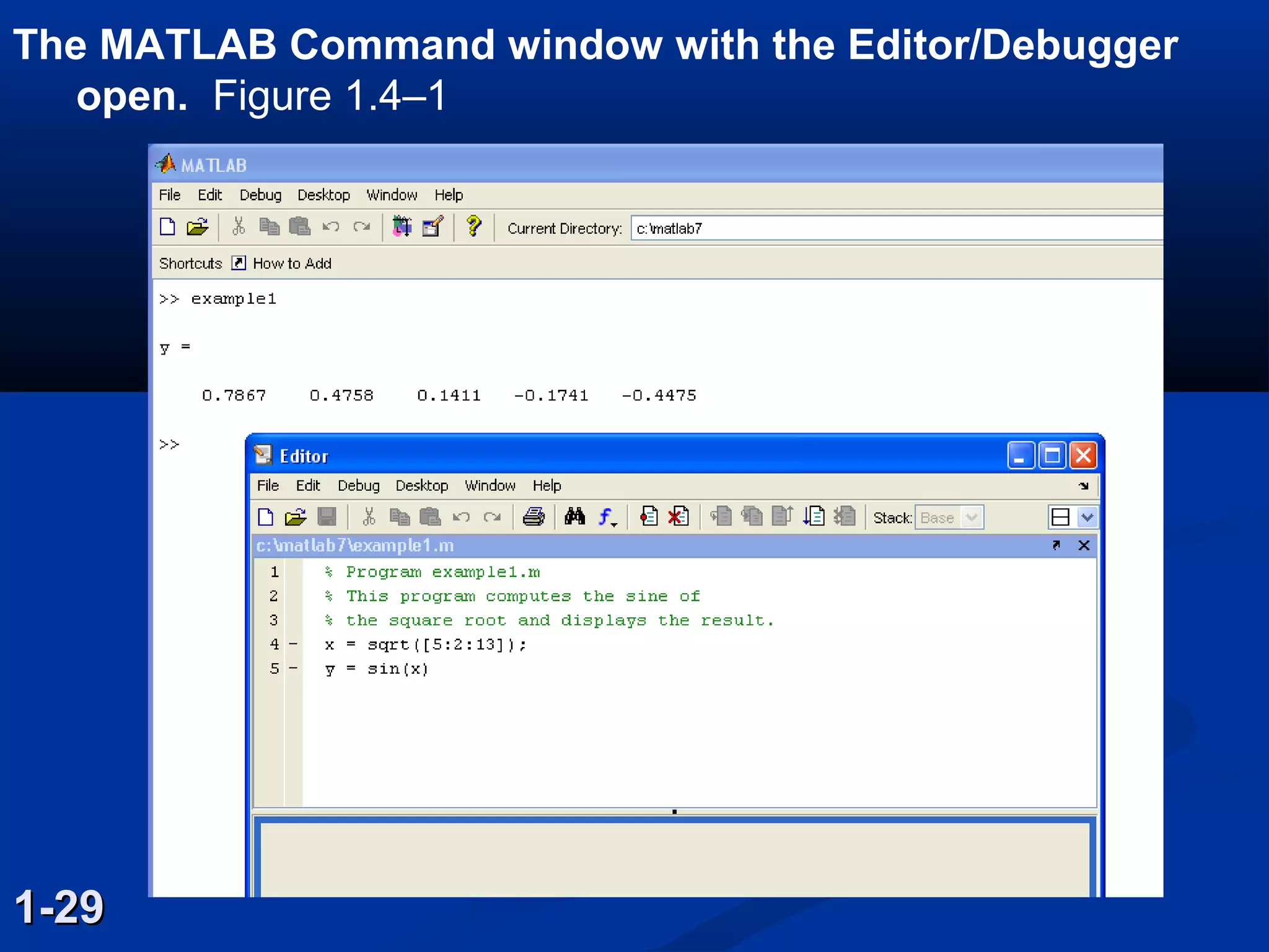
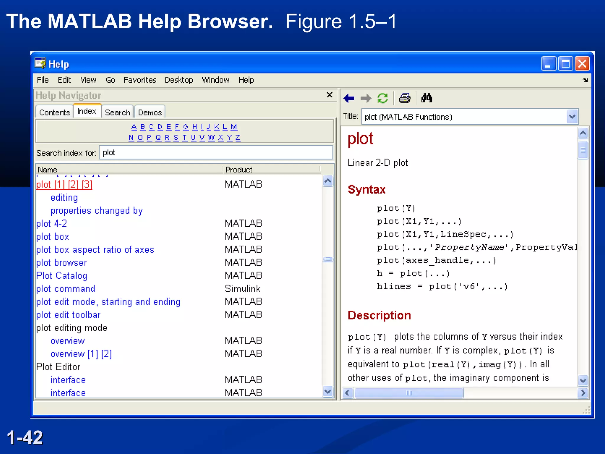
46. The MATLAB Command window with the Editor/Debugger
open. Figure 1.4–1
1-291-29

47. Keep in mind when using script files:
1. The name of a script file must begin with a letter, and
may include digits and the underscore character, up to
31 characters.
2. Do not give a script file the same name as a variable.
3. Do not give a script file the same name as a MATLAB
command or function. You can check to see if a
command, function or file name already exists by using
the exist command.
1-30

48. Debugging Script Files
Program errors usually fall into one of the
following categories.
1. Syntax errors such as omitting a parenthesis
or comma, or spelling a command name
incorrectly. MATLAB usually detects the
more obvious errors and displays a message
describing the error and its location.
2. Errors due to an incorrect mathematical
procedure, called runtime errors. Their
occurrence often depends on the particular
input data. A common example is division by
zero.
1-311-31

49. To locate program errors, try the following:
1. Test your program with a simple version of
the problem which can be checked by hand.
2. Display any intermediate calculations by
removing semicolons at the end of
statements.
3. Use the debugging features of the
Editor/Debugger.
1-321-32

50. Programming Style
1. Comments section
a. The name of the program and any key
words in the first line.
b. The date created, and the creators' names
in the second line.
c. The definitions of the variable names for
every input and output variable. Include
definitions of variables used in the calculations
and units of measurement for all input and all
output variables!
d. The name of every user-defined function
called by the program.
1-331-33 (continued …)

51. 2. Input section Include input data
and/or the input functions and
comments for documentation.
3. Calculation section
4. Output section This section might
contain functions for displaying the
output on the screen.
Programming Style (continued)
1-34

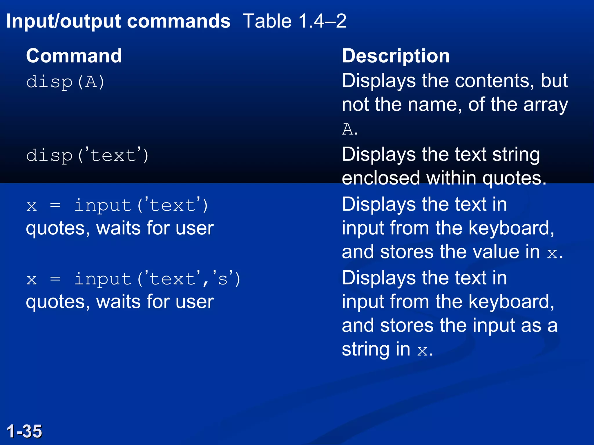
52. Input/output commands Table 1.4–2
1-351-35
Command Description
disp(A) Displays the contents, but
not the name, of the array
A.
disp(’text’) Displays the text string
enclosed within quotes.
x = input(’text’) Displays the text in
quotes, waits for user input from the keyboard,
and stores the value in x.
x = input(’text’,’s’) Displays the text in
quotes, waits for user input from the keyboard,
and stores the input as a
string in x.

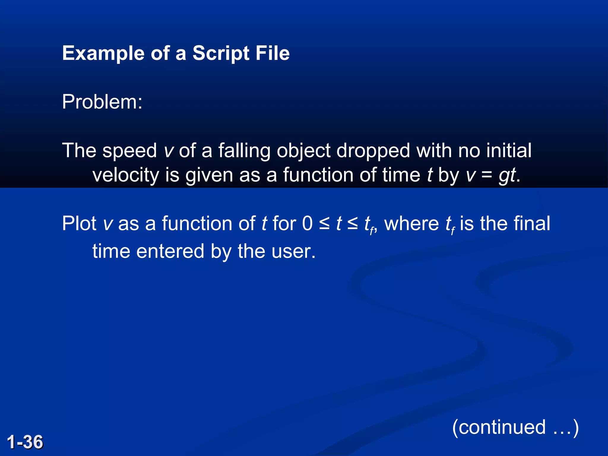
53. Example of a Script File
Problem:
The speed v of a falling object dropped with no initial
velocity is given as a function of time t by v = gt.
Plot v as a function of t for 0 ≤ t ≤ tf, where tf is the final
time entered by the user.
1-361-36
(continued …)

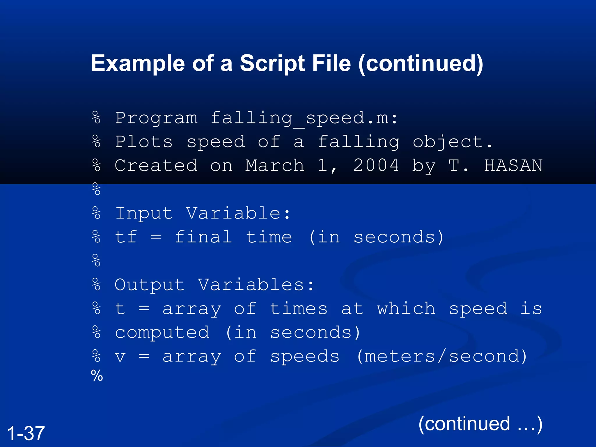
54. Example of a Script File (continued)
% Program falling_speed.m:
% Plots speed of a falling object.
% Created on March 1, 2004 by T. HASAN
%
% Input Variable:
% tf = final time (in seconds)
%
% Output Variables:
% t = array of times at which speed is
% computed (in seconds)
% v = array of speeds (meters/second)
%
(continued …)
1-37

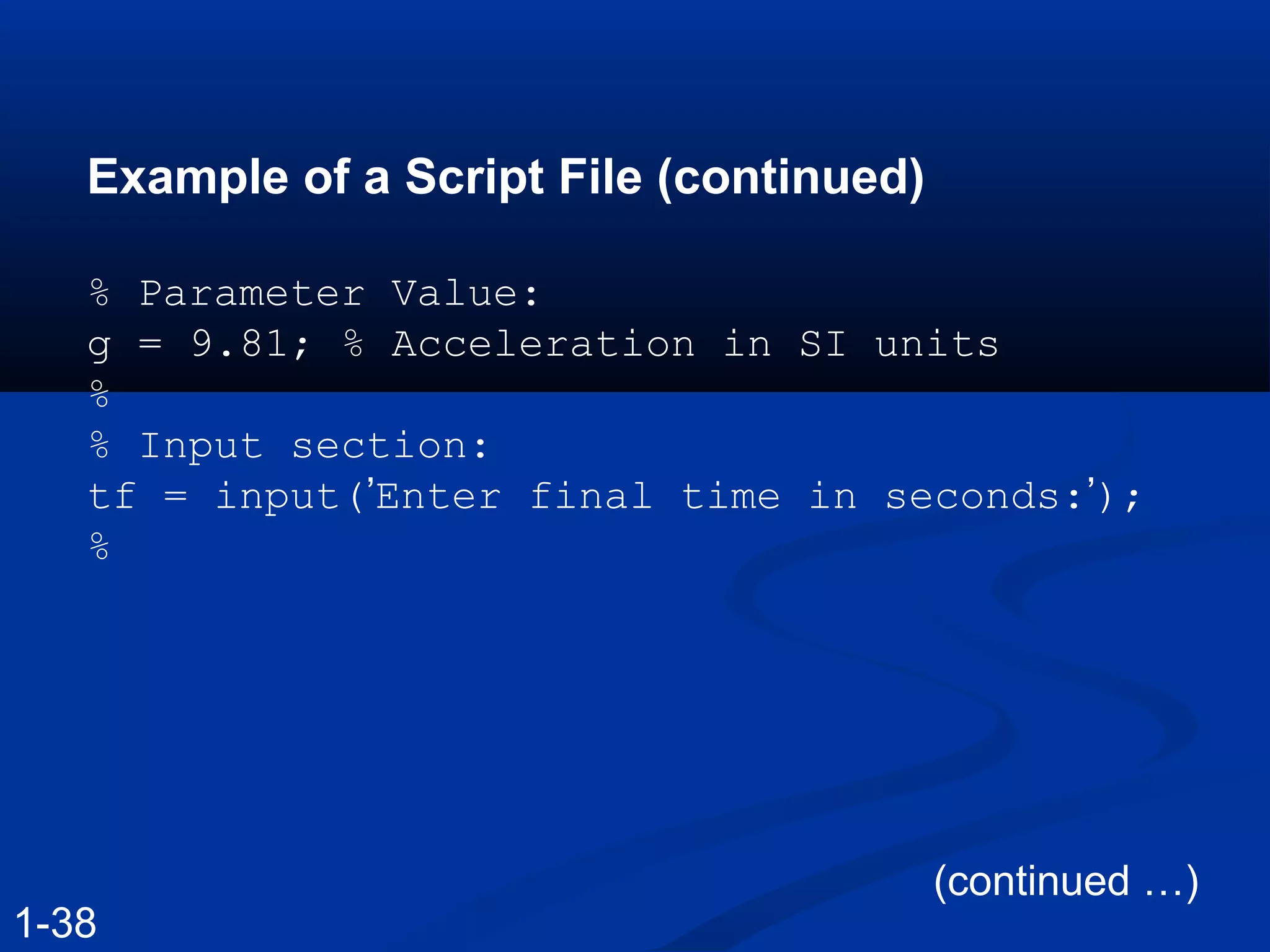
55. Example of a Script File (continued)
% Parameter Value:
g = 9.81; % Acceleration in SI units
%
% Input section:
tf = input(’Enter final time in seconds:’);
%
(continued …)
1-38

56. Example of a Script File (continued)
% Calculation section:
dt = tf/500;
% Create an array of 501 time values.
t = [0:dt:tf];
% Compute speed values.
v = g*t;
%
% Output section:
Plot(t,v),xlabel(’t (s)’),ylabel(’v m/s)’)
1-391-39

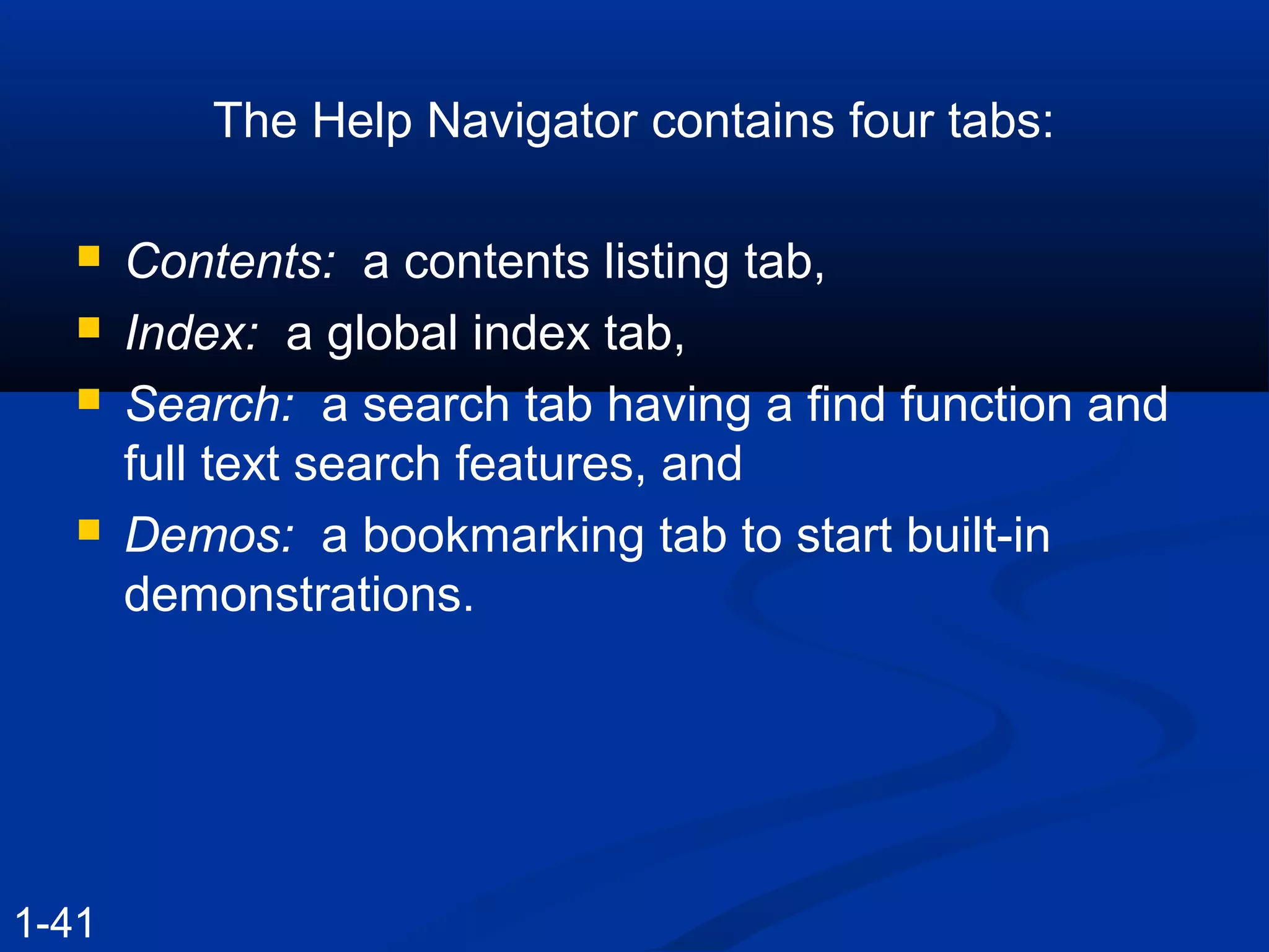
57. The Help Navigator contains four tabs:
 Contents: a contents listing tab,
 Index: a global index tab,
 Search: a search tab having a find function and
full text search features, and
 Demos: a bookmarking tab to start built-in
demonstrations.
1-41

58. The MATLAB Help Browser. Figure 1.5–1
1-421-42

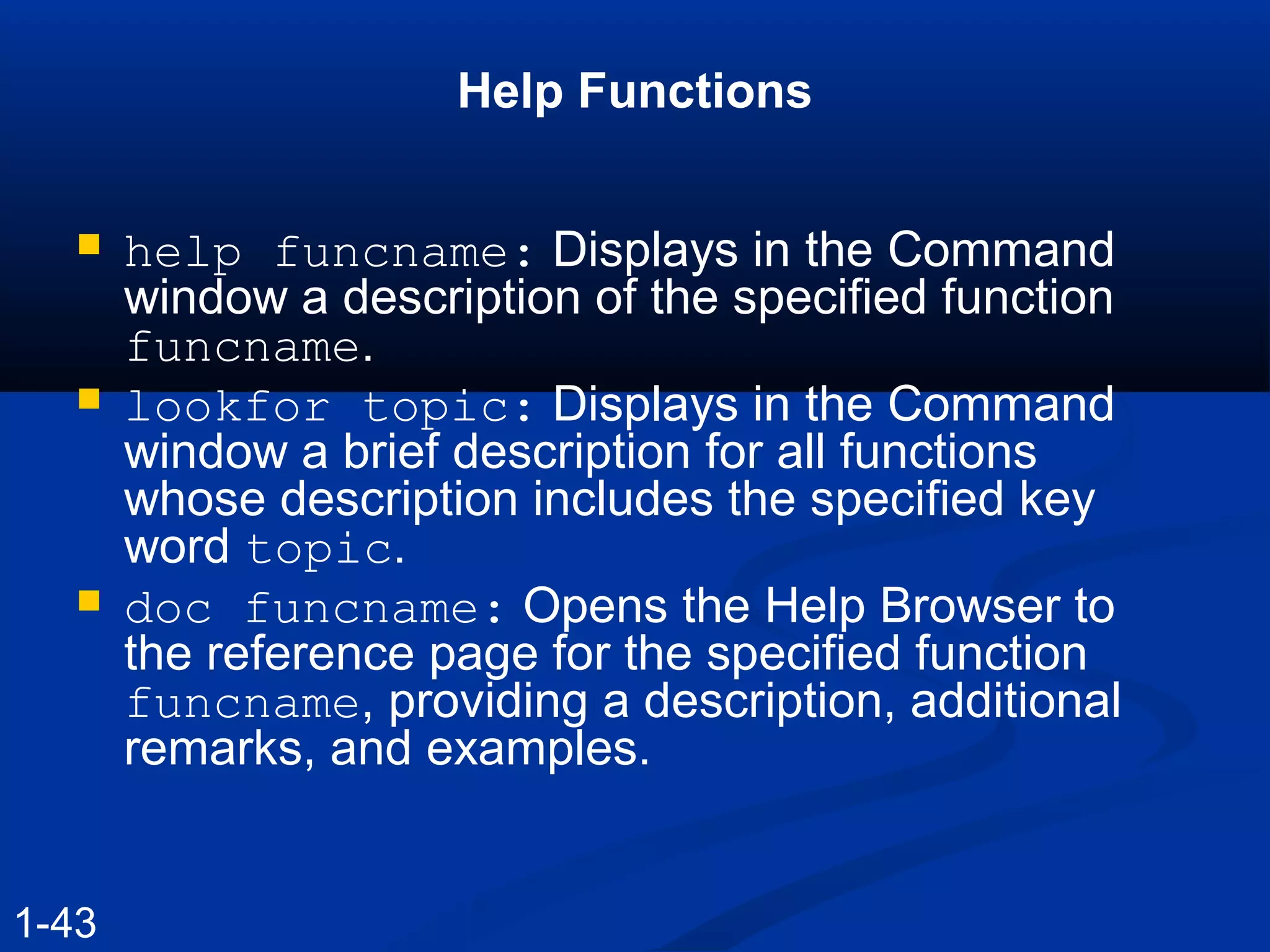
59. Help Functions
 help funcname: Displays in the Command
window a description of the specified function
funcname.
 lookfor topic: Displays in the Command
window a brief description for all functions
whose description includes the specified key
word topic.
 doc funcname: Opens the Help Browser to
the reference page for the specified function
funcname, providing a description, additional
remarks, and examples.
1-43

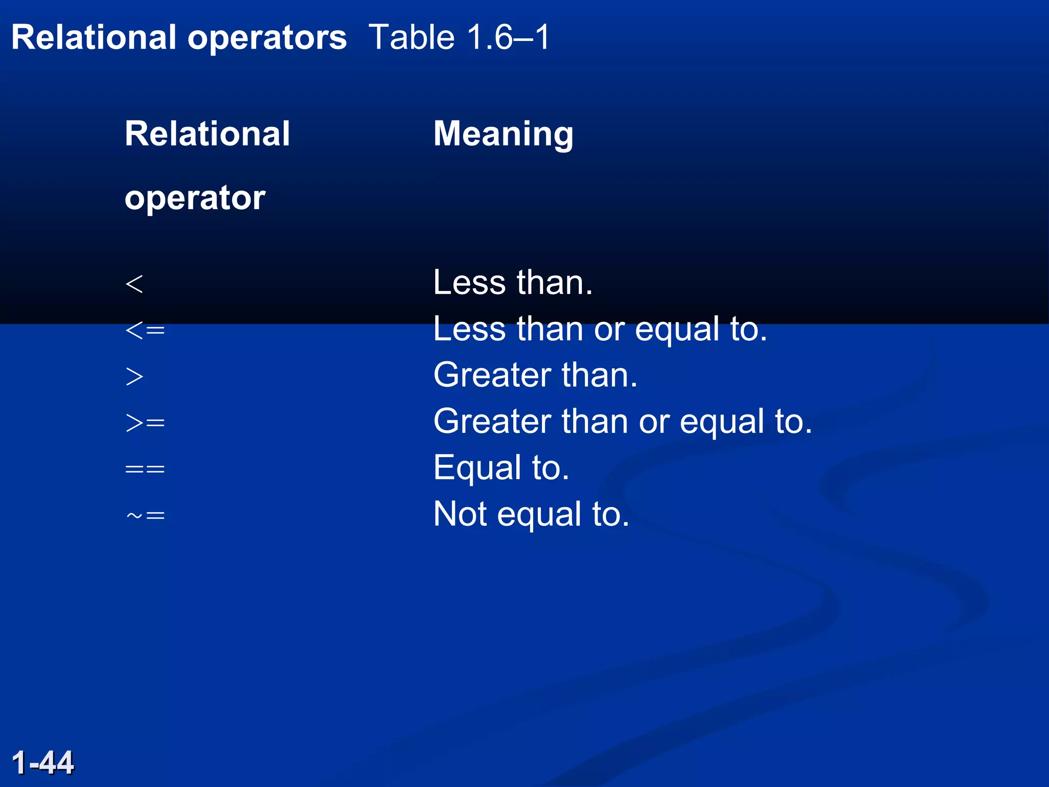
60. Relational operators Table 1.6–1
1-441-44
Relational Meaning
operator
< Less than.
<= Less than or equal to.
> Greater than.
>= Greater than or equal to.
== Equal to.
~= Not equal to.

61. Examples of Relational Operators
>> x = [6,3,9]; y = [14,2,9];
>> z = (x < y)
z =
1 0 0
>>z = ( x > y)
z =
0 1 0
>>z = (x ~= y)
z =
1 1 0
>>z = ( x == y)
z =
0 0 1
>>z = (x > 8)
z =
0 0 11-451-45

62. The find Function
find(x) computes an array containing the indices of the
nonzero elements of the numeric array x. For example
>>x = [-2, 0, 4];
>>y = find(x)
Y =
1 3
The resulting array y = [1, 3] indicates that the first
and third elements of x are nonzero.
1-461-46

63. Note the difference between the result obtained by
x(x<y) and the result obtained by find(x<y).
>>x = [6,3,9,11];y = [14,2,9,13];
>>values = x(x<y)
values =
6 11
>>how_many = length(values)
how_many =
2
>>indices = find(x<y)
indices =
1 4
1-471-47 More? See pages 45-46.

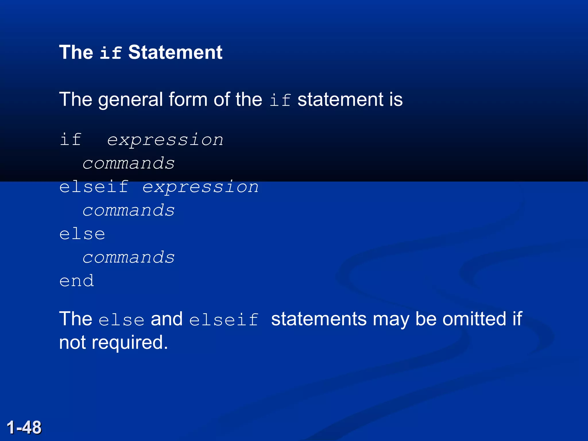
64. The if Statement
The general form of the if statement is
if expression
commands
elseif expression
commands
else
commands
end
The else and elseif statements may be omitted if
not required.
1-481-48

65. 1-491-49
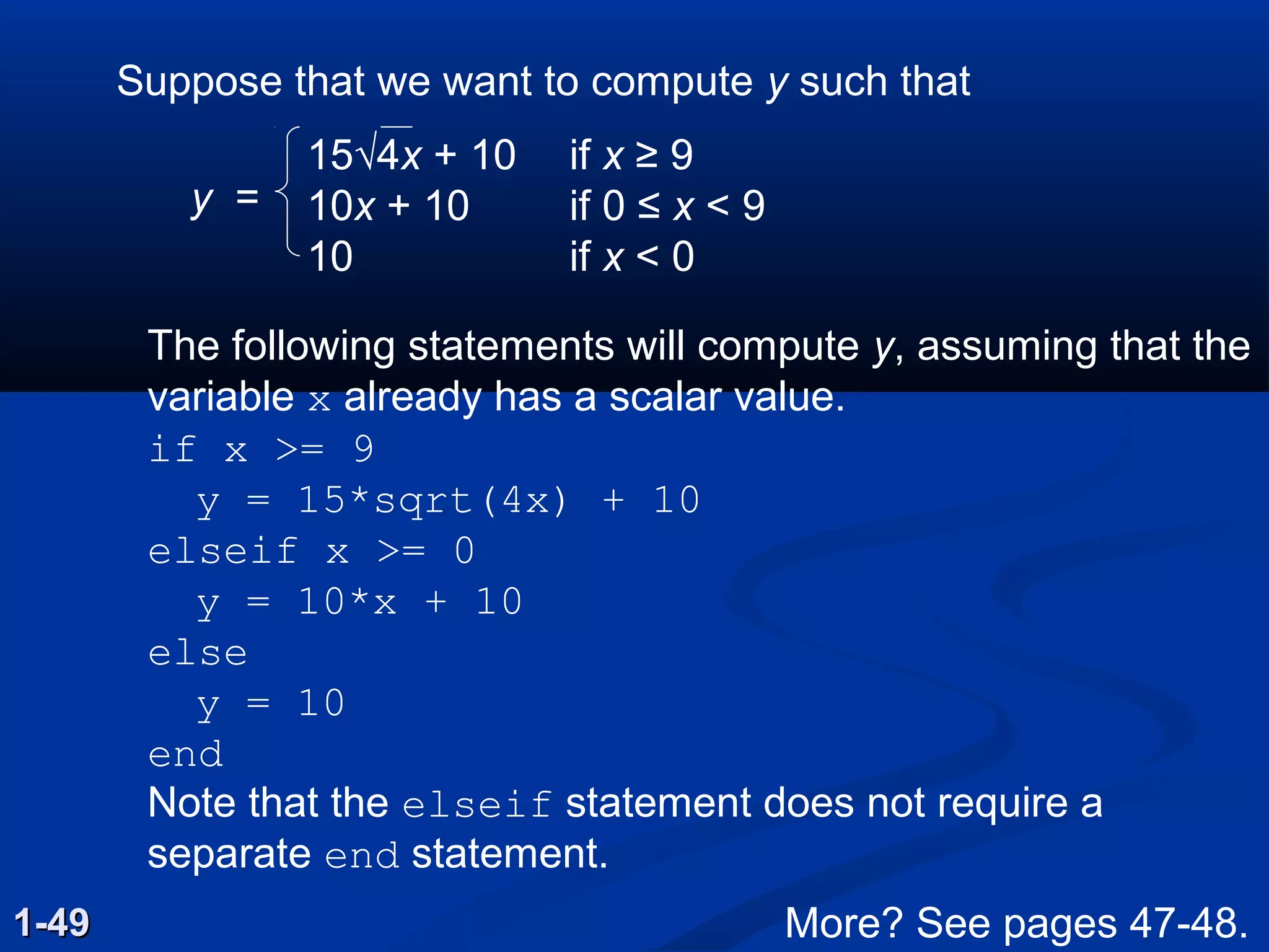
Suppose that we want to compute y such that
15√4x + 10 if x ≥ 9
10x + 10 if 0 ≤ x < 9
10 if x < 0
The following statements will compute y, assuming that the
variable x already has a scalar value.
if x >= 9
y = 15*sqrt(4x) + 10
elseif x >= 0
y = 10*x + 10
else
y = 10
end
Note that the elseif statement does not require a
separate end statement.
y =
More? See pages 47-48.

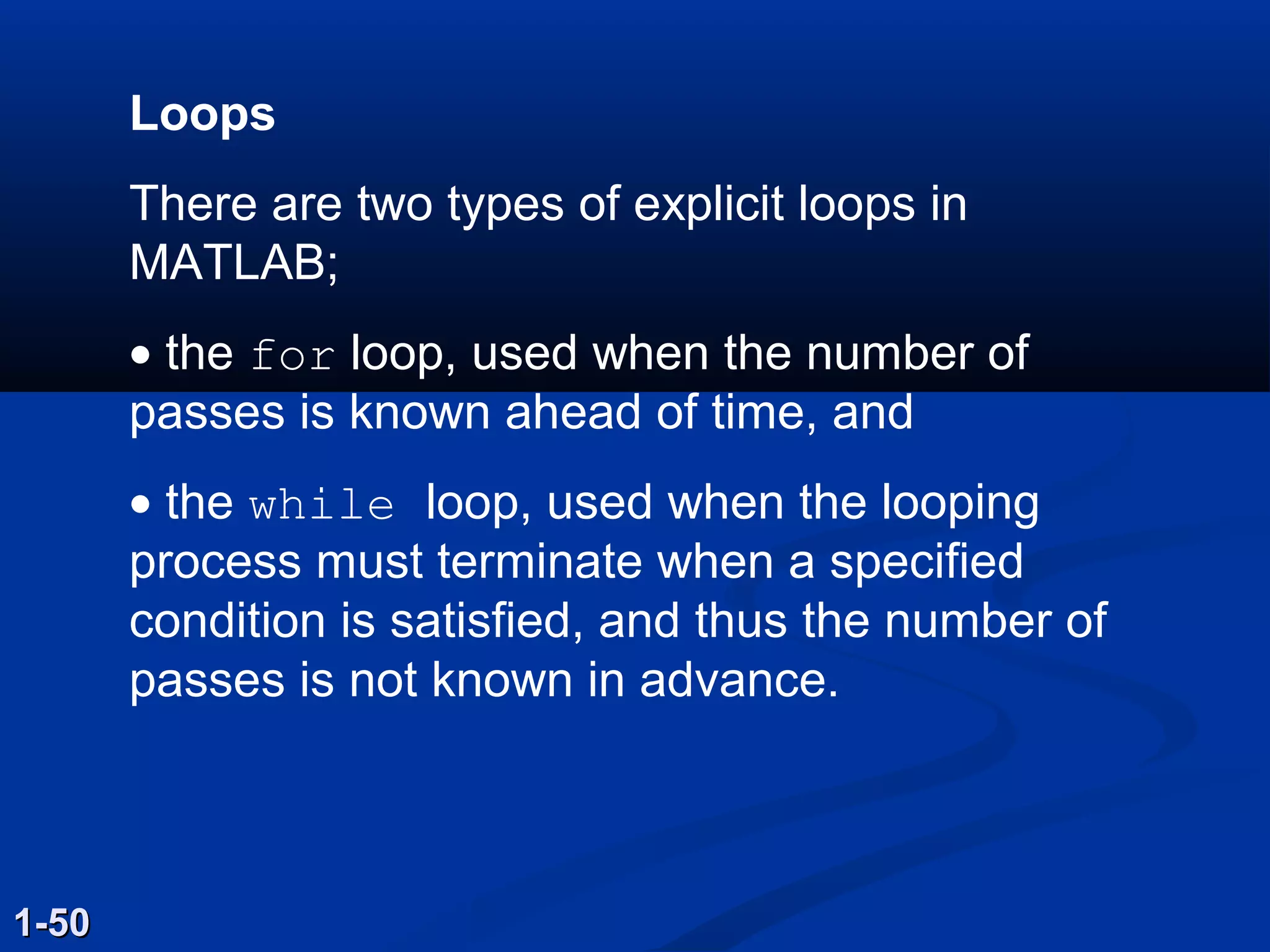
66. Loops
There are two types of explicit loops in
MATLAB;
• the for loop, used when the number of
passes is known ahead of time, and
• the while loop, used when the looping
process must terminate when a specified
condition is satisfied, and thus the number of
passes is not known in advance.
1-501-50

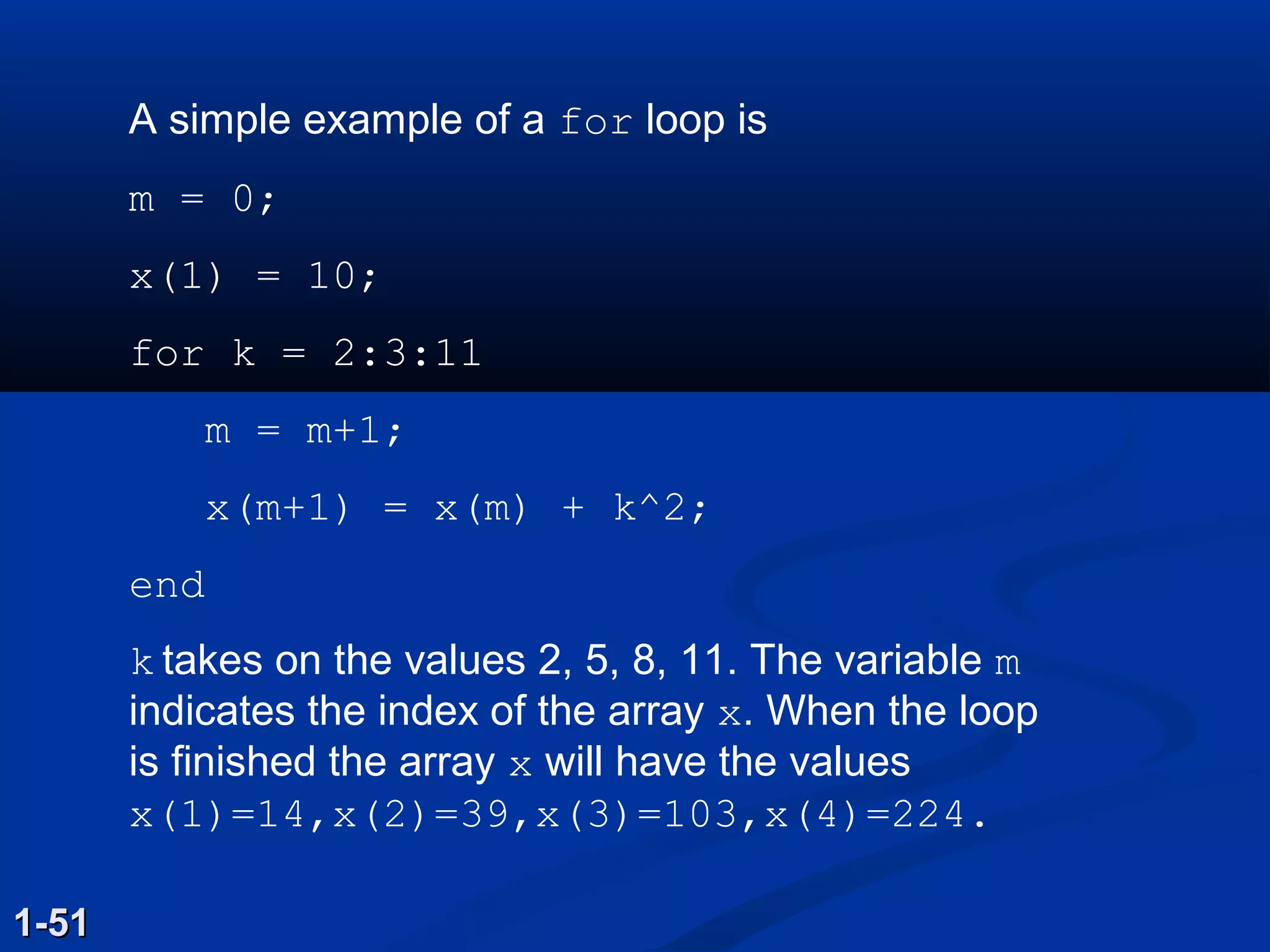
67. A simple example of a for loop is
m = 0;
x(1) = 10;
for k = 2:3:11
m = m+1;
x(m+1) = x(m) + k^2;
end
k takes on the values 2, 5, 8, 11. The variable m
indicates the index of the array x. When the loop
is finished the array x will have the values
x(1)=14,x(2)=39,x(3)=103,x(4)=224.
1-511-51

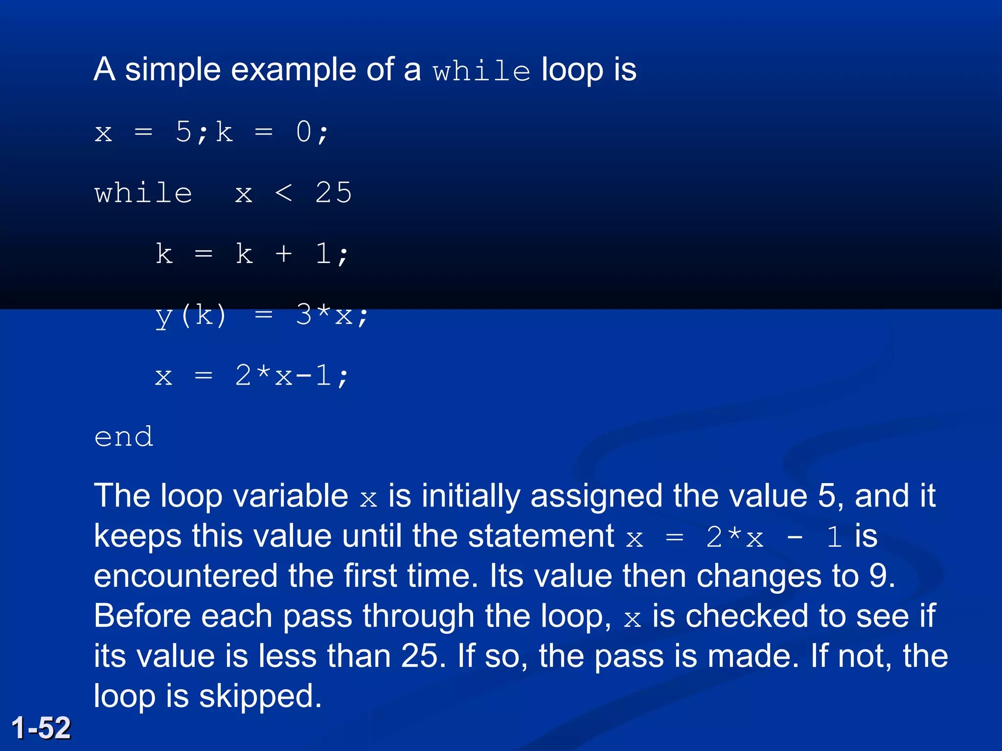
68. A simple example of a while loop is
x = 5;k = 0;
while x < 25
k = k + 1;
y(k) = 3*x;
x = 2*x-1;
end
The loop variable x is initially assigned the value 5, and it
keeps this value until the statement x = 2*x - 1 is
encountered the first time. Its value then changes to 9.
Before each pass through the loop, x is checked to see if
its value is less than 25. If so, the pass is made. If not, the
loop is skipped.
1-521-52

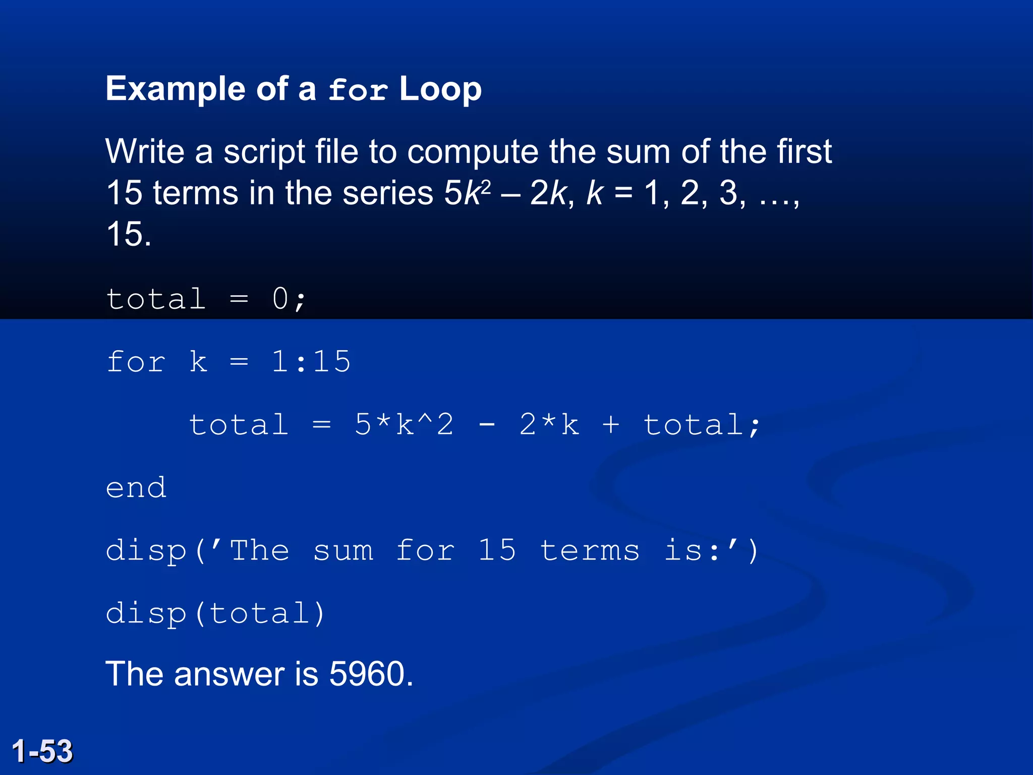
69. Example of a for Loop
Write a script file to compute the sum of the first
15 terms in the series 5k2
– 2k, k = 1, 2, 3, …,
15.
total = 0;
for k = 1:15
total = 5*k^2 - 2*k + total;
end
disp(’The sum for 15 terms is:’)
disp(total)
The answer is 5960.
1-531-53

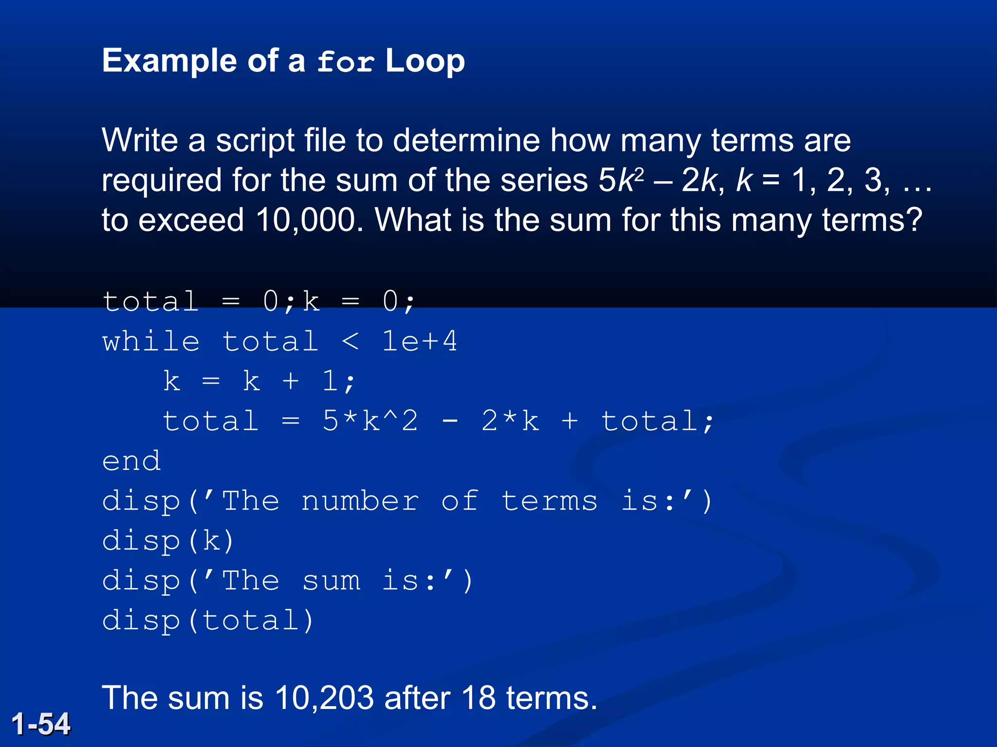
70. Example of a for Loop
Write a script file to determine how many terms are
required for the sum of the series 5k2
– 2k, k = 1, 2, 3, …
to exceed 10,000. What is the sum for this many terms?
total = 0;k = 0;
while total < 1e+4
k = k + 1;
total = 5*k^2 - 2*k + total;
end
disp(’The number of terms is:’)
disp(k)
disp(’The sum is:’)
disp(total)
The sum is 10,203 after 18 terms.
1-541-54

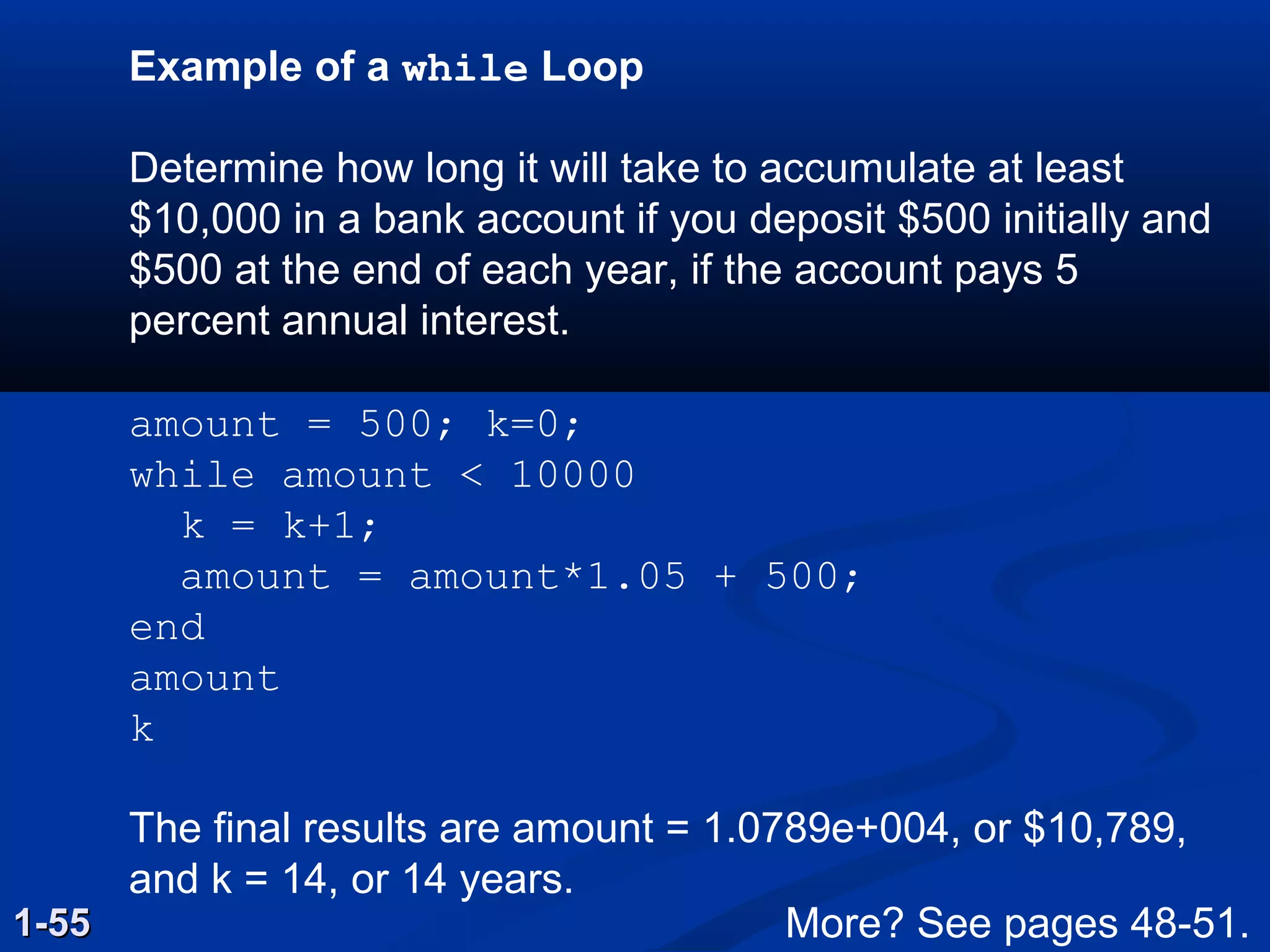
71. Example of a while Loop
Determine how long it will take to accumulate at least
$10,000 in a bank account if you deposit $500 initially and
$500 at the end of each year, if the account pays 5
percent annual interest.
amount = 500; k=0;
while amount < 10000
k = k+1;
amount = amount*1.05 + 500;
end
amount
k
The final results are amount = 1.0789e+004, or $10,789,
and k = 14, or 14 years.
1-551-55 More? See pages 48-51.

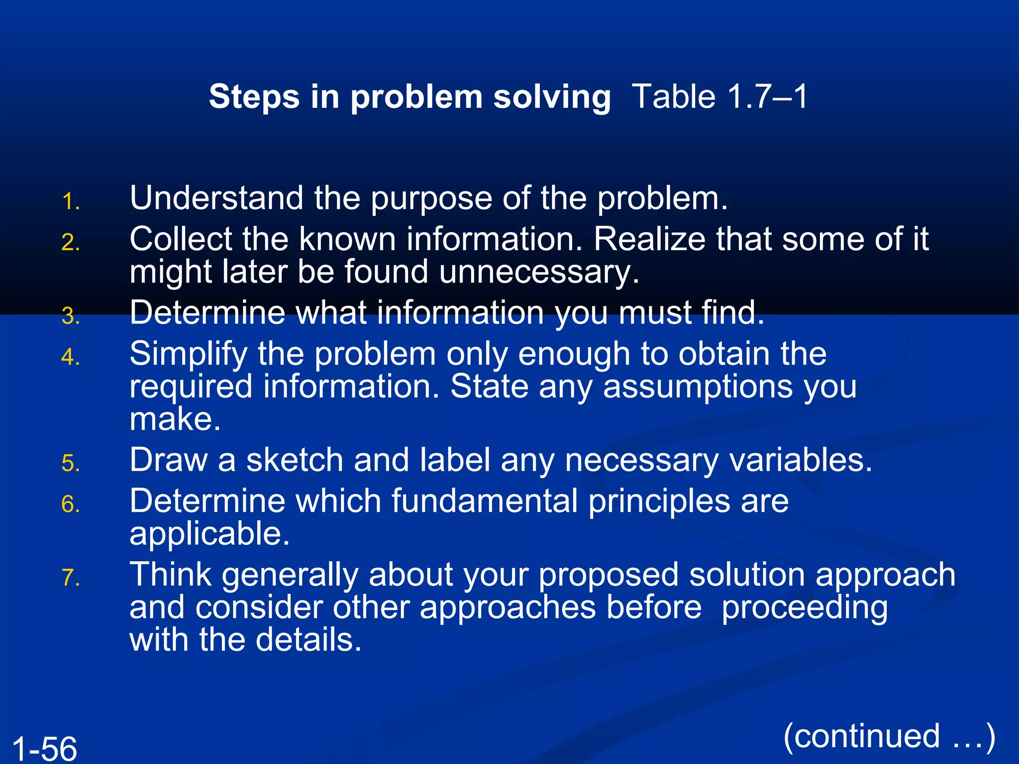
72. Steps in problem solving Table 1.7–1
1. Understand the purpose of the problem.
2. Collect the known information. Realize that some of it
might later be found unnecessary.
3. Determine what information you must find.
4. Simplify the problem only enough to obtain the
required information. State any assumptions you
make.
5. Draw a sketch and label any necessary variables.
6. Determine which fundamental principles are
applicable.
7. Think generally about your proposed solution approach
and consider other approaches before proceeding
with the details.
(continued …)1-56

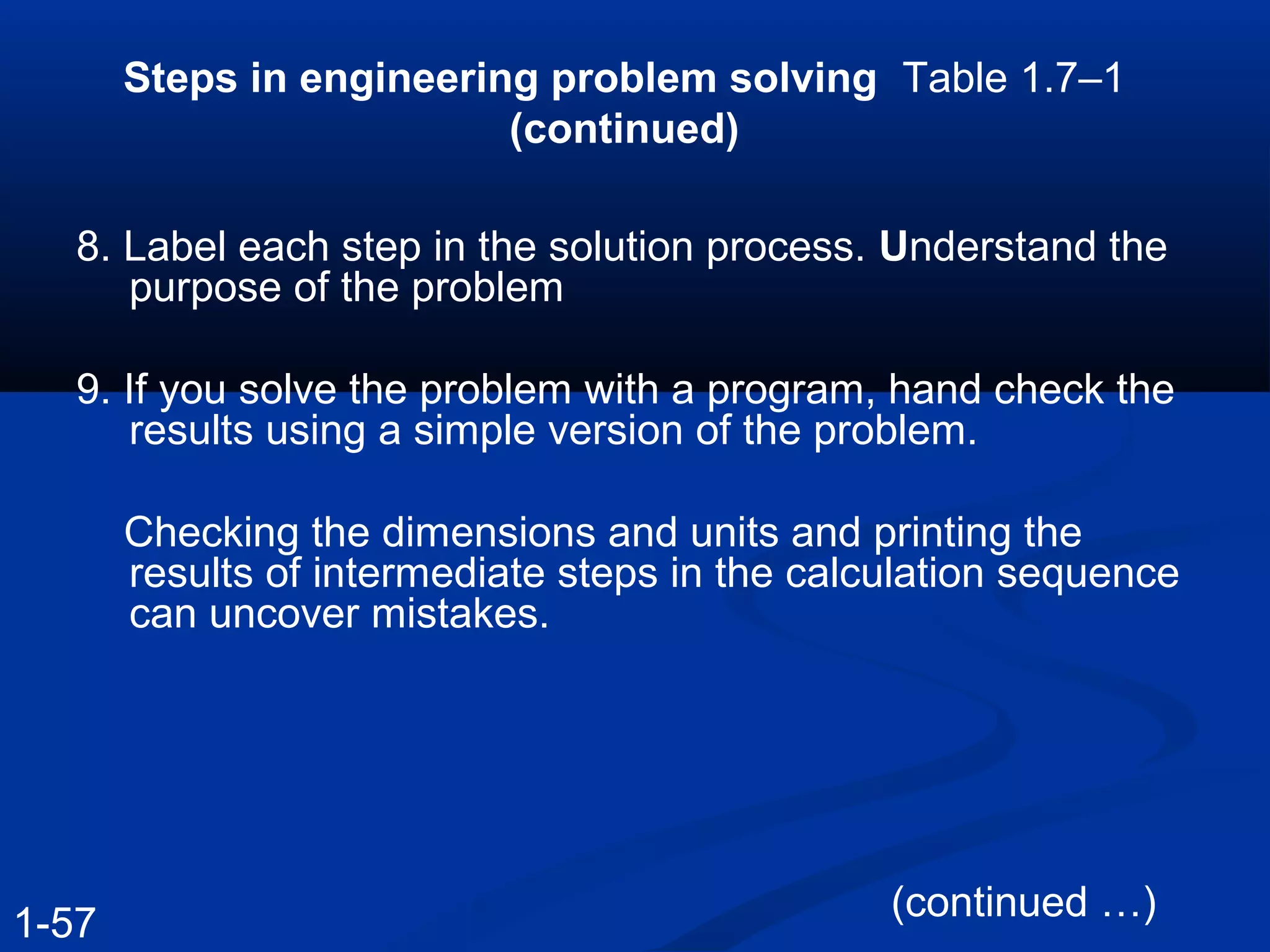
73. Steps in engineering problem solving Table 1.7–1
(continued)
8. Label each step in the solution process. Understand the
purpose of the problem
9. If you solve the problem with a program, hand check the
results using a simple version of the problem.
Checking the dimensions and units and printing the
results of intermediate steps in the calculation sequence
can uncover mistakes.
(continued …)
1-57

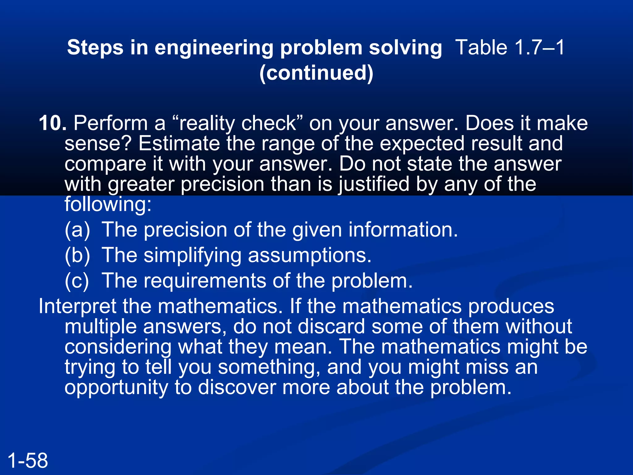
74. Steps in engineering problem solving Table 1.7–1
(continued)
10. Perform a “reality check” on your answer. Does it make
sense? Estimate the range of the expected result and
compare it with your answer. Do not state the answer
with greater precision than is justified by any of the
following:
(a) The precision of the given information.
(b) The simplifying assumptions.
(c) The requirements of the problem.
Interpret the mathematics. If the mathematics produces
multiple answers, do not discard some of them without
considering what they mean. The mathematics might be
trying to tell you something, and you might miss an
opportunity to discover more about the problem.
1-58

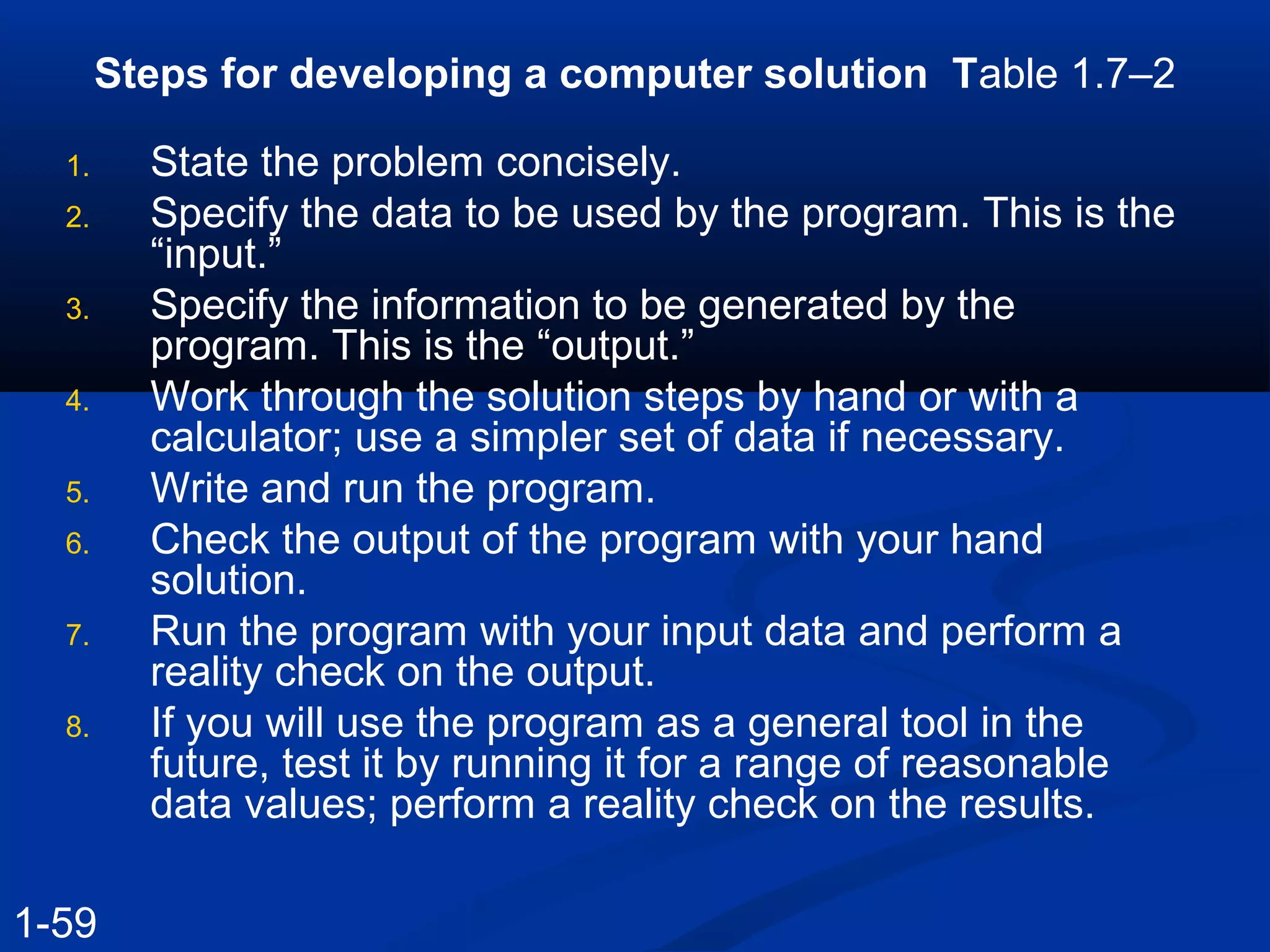
75. Steps for developing a computer solution Table 1.7–2
1. State the problem concisely.
2. Specify the data to be used by the program. This is the
“input.”
3. Specify the information to be generated by the
program. This is the “output.”
4. Work through the solution steps by hand or with a
calculator; use a simpler set of data if necessary.
5. Write and run the program.
6. Check the output of the program with your hand
solution.
7. Run the program with your input data and perform a
reality check on the output.
8. If you will use the program as a general tool in the
future, test it by running it for a range of reasonable
data values; perform a reality check on the results.
1-59

76. Assignment 1Assignment 1
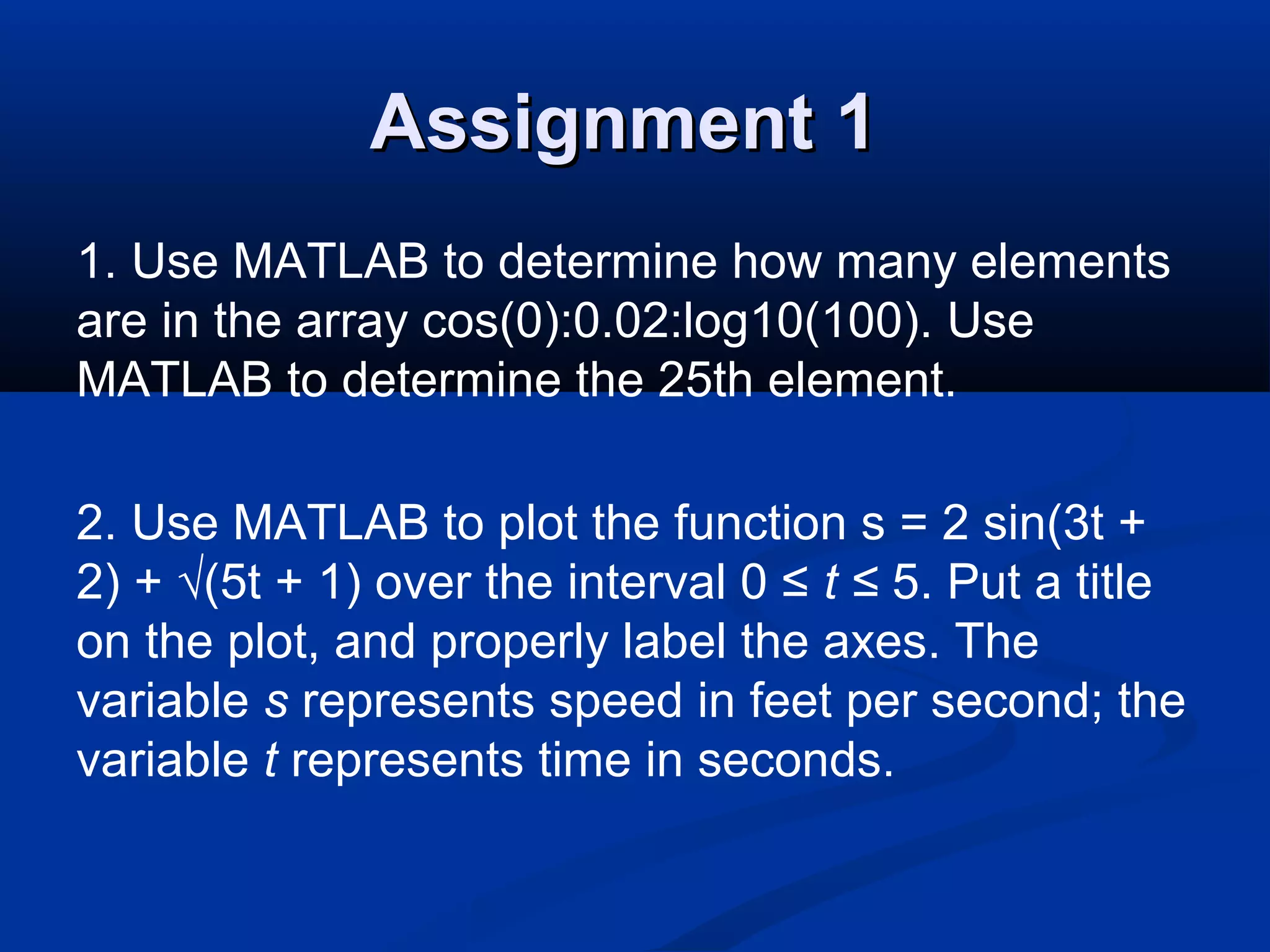
1. Use MATLAB to determine how many elements
are in the array cos(0):0.02:log10(100). Use
MATLAB to determine the 25th element.
2. Use MATLAB to plot the function s = 2 sin(3t +
2) + √(5t + 1) over the interval 0 ≤ t ≤ 5. Put a title
on the plot, and properly label the axes. The
variable s represents speed in feet per second; the
variable t represents time in seconds.

77. Assignment 1Assignment 1
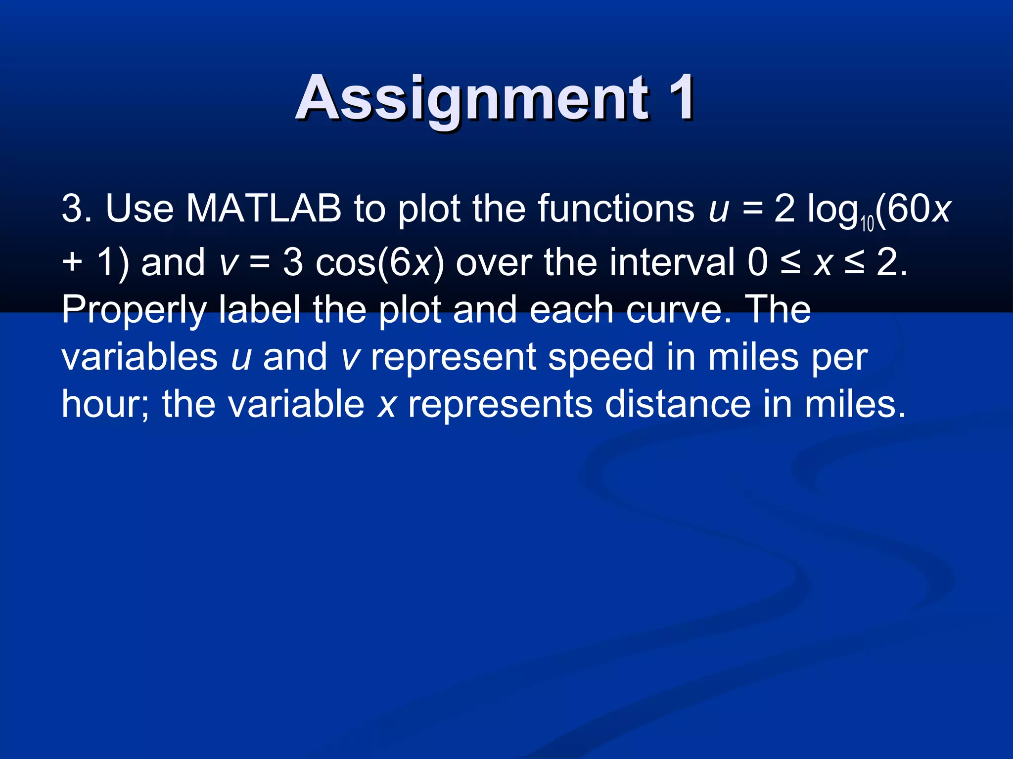
3. Use MATLAB to plot the functions u = 2 log10(60x
+ 1) and v = 3 cos(6x) over the interval 0 ≤ x ≤ 2.
Properly label the plot and each curve. The
variables u and v represent speed in miles per
hour; the variable x represents distance in miles.