Adv math[unit 2]

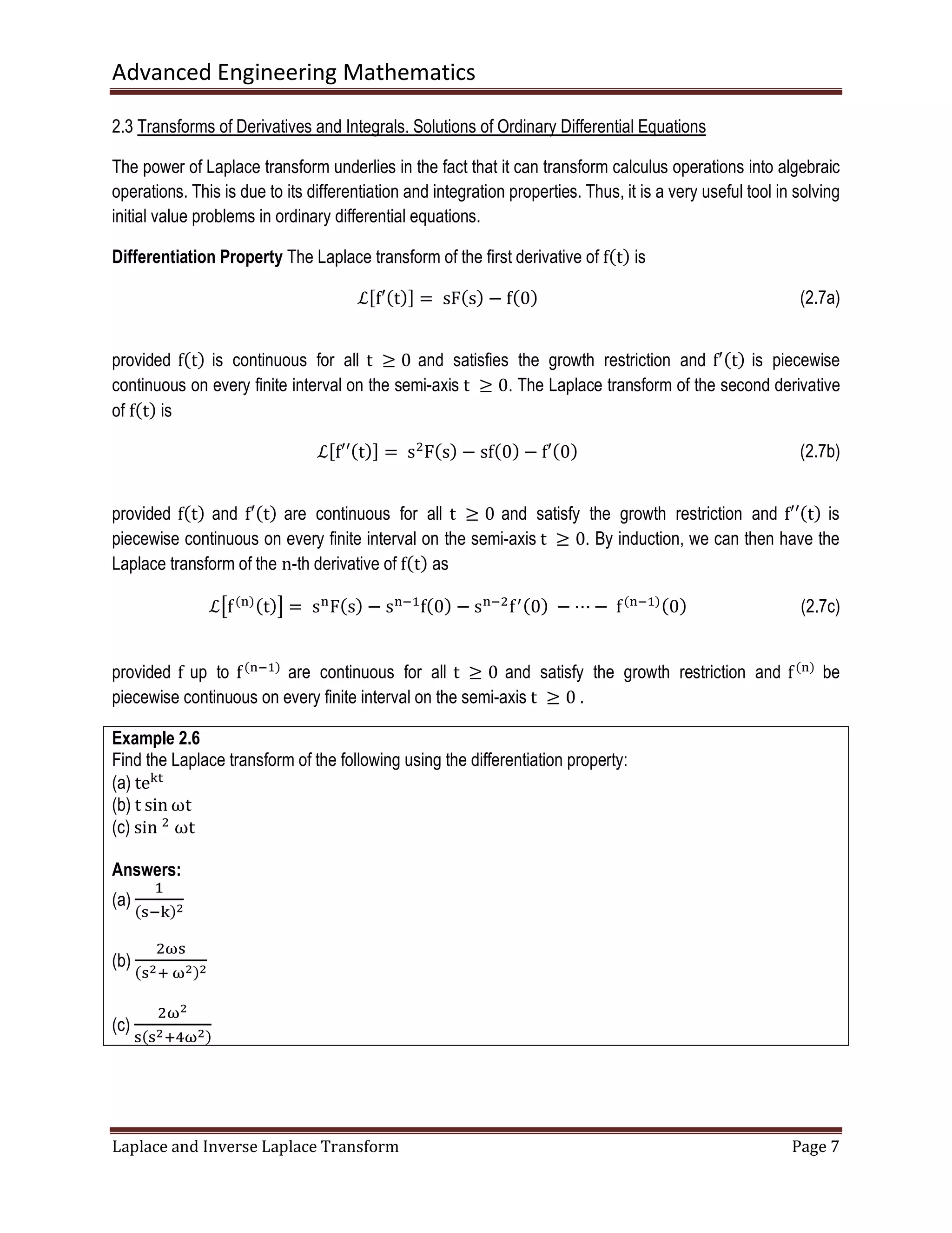
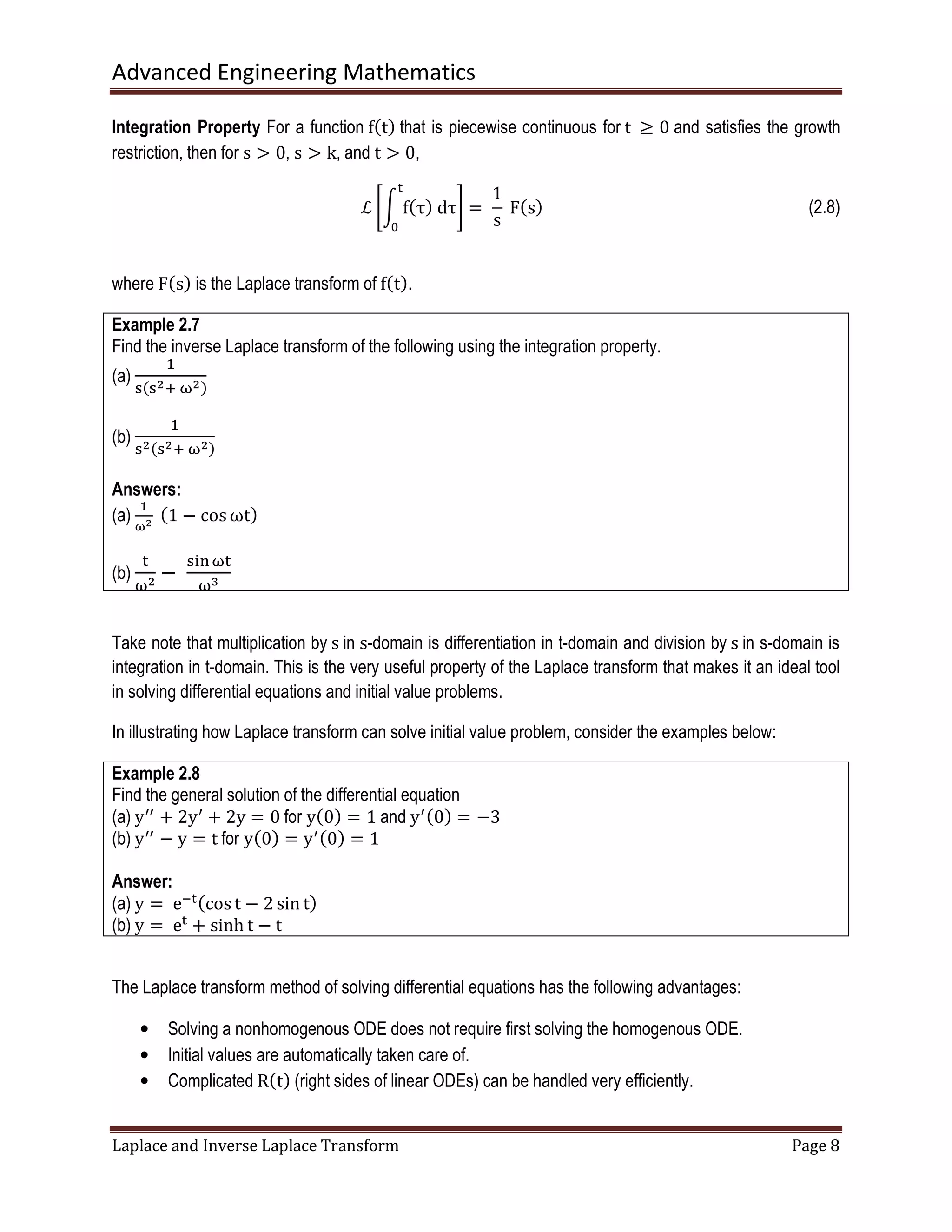
Advanced Engineering Mathematics
Laplace and Inverse Laplace Transform Page 1
LAPLACE AND INVERSE LAPLACE TRANSFORM
The Laplace transforms and its inverse has many important applications in mathematics, physics,
economics, engineering, and probability theory. Pierre Simon Marquis de Laplace originally developed the
integral transform for his work on the probability theory. However, the powerful, practical Laplace transform
techniques were developed only a century later by Oliver Heaviside.
The Laplace transform, because of its properties, makes solving ordinary differential equations much easier
by making operations in calculus algebraic. Moreover, compared to other transform techniques (such as
Fourier transform), the Laplace transform virtually exists to almost all kinds of functions, subject to certain
restrictions. It is then ideal to use Laplace transform to analyze systems modeled by differential equations
and are causal in nature.
2.1 Definition, Existence and Uniqueness of the Laplace Transform
Let fሺtሻ be a causal function, so fሺtሻ = 0 for t < 0. The Laplace transform Fሺsሻ of fሺtሻ is the complex
function defined for s ∈ ℂ by
Fሺsሻ = න eିୱ୲
fሺtሻ dt
ஶ
଴
(2.1)
provided that the integral exists.
The Laplace transform basically maps the function fሺtሻ, which is in t-domain (in applications, time-domain)
into s-domain (which we will call later as the complex frequency domain). We shall use the following
notation
ℒሺfሻ = Fሺsሻ (2.2a)
read as the Laplace transform of the function fሺtሻ is the function Fሺsሻ, and
ℒିଵሺFሻ = fሺtሻ (2.2b)
which denotes the inverse Laplace transform of the function Fሺsሻ is the function fሺtሻ. Also take note that
the original functions fሺtሻ depend on t and their transforms Fሺsሻ depend on s. We shall use lowercase
letter for the original functions and the same letter in upper case to denote their transforms.
In Eq. 2.1 we need to evaluate the integral from zero to infinity; such integrals are called improper integrals.
Improper integrals are evaluated according to the rule
න eିୱ୲
fሺtሻ dt
ஶ
଴
= lim
୘→ஶ
න eିୱ୲
fሺtሻ dt
୘
଴
(2.3)

Note that the function fሺtሻ must be causal, that is its value is fሺtሻ when t ൒ 0 and 0 when t < 0.
Example 2.1
Using the Laplace integral, find the Laplace transform of the following:
(a) fሺtሻ = 1
(b) fሺtሻ = eୟ୲
, a is a constant
(c) fሺtሻ = t
(d) fሺtሻ = cos ωt, ω is a constant
(e) fሺtሻ = sin ωt, ω is a constant
Answers:
(a) Fሺsሻ =
ଵ
ୱ
(b) Fሺsሻ =
ଵ
ୱିୟ
(c) Fሺsሻ =
ଵ
ୱమ
(d) Fሺsሻ =
ୱ
ୱమା னమ
(e) Fሺsሻ =
ன
ୱమା னమ
A function fሺtሻ has a Laplace transform if it does not grow too fast, say, if for all t ≧ 0 and some constants
M and k it satisfies the growth restriction
|fሺtሻ| ≦ Me୩୲ (2.4)
The function fሺtሻ also need not to be continuous in the whole interval, rather it should be piecewise
continuous. A function is piecewise continuous on a finite interval a ൑ t ൑ b where f is defined, if this
interval can be divided into finitely many subintervals in each of which f is continuous and has finite limit as
t approaches either endpoint of such a subinterval from the interior.. Figure 2.1 illustrates a piecewise
continuous function as an example.
Figure 2.1. A Piecewise Continuous Function
We can now state the existence of the Laplace transform in the following manner: if fሺtሻ is defined and
piecewise continuous on every finite interval on the semi-axis t ൒ 0 and satisfies the growth restriction
(Eq. 2.4) for all t ൒ 0 and some constants M and k then the Laplace transform ℒሺfሻ exists for all s ൐ k.

It can also be seen that when the Laplace transform of a given function exists, it is uniquely determined. In
the same manner, the inverse of a given transform is essentially unique.
2.2 General Properties of Laplace Transform: Linearity, s-shifting. Table of Laplace Transform.
Because of some basic properties and the uniqueness of Laplace transform, we can deviate from using the
Laplace integral to all functions. All we need is to derive the Laplace transform of basic functions then apply
the properties. At the end of this section, a table of Laplace transform is presented.
Linearity Just as differentiation and integration are linear, Laplace transform is also a linear operation, that
is for any functions fሺtሻ and gሺtሻ whose transforms exist and any constants a and b, the transform of
afሺtሻ + bgሺtሻ exists and
ℒሾafሺtሻ + bgሺtሻሿ = aℒሾfሺtሻሿ + bℒሾgሺtሻሿ = aFሺsሻ + bGሺsሻ (2.5)
Example 2.2
Using the linearity theorem, and the previously obtained Laplace transform pairs, find the Laplace
transforms of
(a) cosh at
(b) sinh at
(c) cos ωt
(d) sin ωt
First shifting theorem: Shifting in the s-domain The Laplace transform has the very useful property that
if we know the transform of fሺtሻ, we can immediately get that of eୟ୲
fሺtሻ, as follows: If fሺtሻ has the
transform Fሺsሻ (where s ൐ k for some k), then eୟ୲
fሺtሻ has the transform Fሺs − aሻ (where s − a ൐ k for
some k). Thus,
ℒሾeୟ୲
fሺtሻሿ = Fሺs − aሻ
eୟ୲
fሺtሻ = ℒିଵሾ Fሺs − aሻሿ
(2.6a)
(2.6b)
Example 2.3
Apply the shifting theorem and the previously obtained Laplace transform pairs to obtain the Laplace
transform of the following:
(a) eୟ୲
cosωt
(b) eୟ୲
sin ωt

The table below shows the Laplace transform pairs we have obtained in the previous examples.
Figure 2.2 Table of Laplace Transform Pairs
We haven’t proved formulas 3, 4 and 5 yet, however, they can be obtained from formula 2 by induction.
Formulas 1 thru 3 are special cases of formula 4 (note that 0! = 1, which applies for formula 1).
Example 2.4
Find the Laplace transform of the following functions using the table (variables other than t are considered
constants)
(a) tଶ
− 2t
(b) cos 2πt
(c) eଶ୲
cosh t
(d) eଷୟିଶୠ୲
(e) cosሺωt + θሻ

Answers
(a)
ଶ
ୱయ
−
ଶ
ୱమ
(b)
ୱ
ୱమାସ஠మ
(c)
ୱିଶ
ሺୱିଶሻమିଵ
(d)
ୣయ౗
ୱାଶୠ
(e)
ୱ ୡ୭ୱ ஘ି னୱ୧୬஘
ୱమା னమ
Example 2.5
Find the inverse Laplace transform of the following functions using the table (variables other than s are
constants)
(a)
ସୱିଷ஠
ୱమା ஠మ
(b)
ୱరିଷୱమାଵଶ
ୱఱ
(c)
ଵହ
ୱమାସୱାଶଽ
(d)
଼
ୱమାସୱ
(e)
ଵ
൫ୱି √ଷ൯൫ୱା√ହ൯
Answers:
(a) 4 cos πt − 3 sin πt
(b) 1 −
ଷ
ଶ
tଶ
+
ଵ
ଶ
tସ
(c) 3eିଶ୲
sin 5t
(d) 2 − 2eିସ୲
(e)
ୣ౪√యି ୣష౪√ఱ
√ଷା √ହ

Drill Problem 2.1
Find the Laplace transform of the following functions. Variables other than t are constants.
1. ሺtଶ
− 3ሻଶ
2. sinଶ
4t
3. eି୲
sinh 5t
4. sin ቀ3t −
ଵ
ଶ
ቁ
5. −8 sin 0.2t
6. sin t cos t
7. ሺt + 1ሻଷ
8. 3.8teଶ.ସ୲
9. −3tସ
eି଴.ହ୲
10. 5eିୟ୲
sin ωt
Find the inverse Laplace transform of the following functions. Variables other than s are constants.
11.
ଵ
ୱమାହ
−
ଵ
ୱାହ
12.
ଶୱାଵ଺
ୱమିଵ଺
13.
ଵ଴
ଶୱା √ଶ
14.
୬஠୐
୐మୱమା ୬మ஠మ
15.
ଶ଴
ሺୱାଵሻሺୱାଷሻ
16.
ଵ଼ୱିଵଶ
ଽୱమିଵ
17.
ଵ
ሺୱାୟሻሺୱାୠሻ
18.
ସୱିଶ
ୱమି଺ୱାଵ଼
19.
஠
ୱమାଵ଴஠ୱାଶସ஠మ
20.
ଶୱିହ଺
ୱమିସୱିଵଶ

2.3 Transforms of Derivatives and Integrals. Solutions of Ordinary Differential Equations
The power of Laplace transform underlies in the fact that it can transform calculus operations into algebraic
operations. This is due to its differentiation and integration properties. Thus, it is a very useful tool in solving
initial value problems in ordinary differential equations.
Differentiation Property The Laplace transform of the first derivative of fሺtሻ is
ℒሾf′ሺtሻሿ = sFሺsሻ − fሺ0ሻ (2.7a)
provided fሺtሻ is continuous for all t ൒ 0 and satisfies the growth restriction and f′ሺtሻ is piecewise
continuous on every finite interval on the semi-axis t ൒ 0. The Laplace transform of the second derivative
of fሺtሻ is
ℒሾf′′ሺtሻሿ = sଶ
Fሺsሻ − sfሺ0ሻ − f′ሺ0ሻ (2.7b)
provided fሺtሻ and f′ሺtሻ are continuous for all t ൒ 0 and satisfy the growth restriction and f′′ሺtሻ is
piecewise continuous on every finite interval on the semi-axis t ൒ 0. By induction, we can then have the
Laplace transform of the n-th derivative of fሺtሻ as
ℒൣfሺ୬ሻሺtሻ൧ = s୬
Fሺsሻ − s୬ିଵ
fሺ0ሻ − s୬ିଶ
fᇱሺ0ሻ − ⋯ − fሺ୬ିଵሻሺ0ሻ (2.7c)
provided f up to fሺ୬ିଵሻ
are continuous for all t ൒ 0 and satisfy the growth restriction and fሺ୬ሻ
be
piecewise continuous on every finite interval on the semi-axis t ൒ 0 .
Example 2.6
Find the Laplace transform of the following using the differentiation property:
(a) te୩୲
(b) t sin ωt
(c) sin ଶ
ωt
Answers:
(a)
ଵ
ሺୱି୩ሻమ
(b)
ଶனୱ
ሺୱమା னమሻమ
(c)
ଶனమ
ୱሺୱమାସனమሻ

Integration Property For a function fሺtሻ that is piecewise continuous for t ൒ 0 and satisfies the growth
restriction, then for s ൐ 0, s ൐ k, and t ൐ 0,
ℒ ቈන fሺτሻ dτ
୲
଴
቉ =
1
s
Fሺsሻ (2.8)
where Fሺsሻ is the Laplace transform of fሺtሻ.
Example 2.7
Find the inverse Laplace transform of the following using the integration property.
(a)
ଵ
ୱሺୱమା னమሻ
(b)
ଵ
ୱమሺୱమା னమሻ
Answers:
(a)
ଵ
னమ ሺ1 − cos ωtሻ
(b)
୲
னమ
−
ୱ୧୬ன୲
னయ
Take note that multiplication by s in s-domain is differentiation in t-domain and division by s in s-domain is
integration in t-domain. This is the very useful property of the Laplace transform that makes it an ideal tool
in solving differential equations and initial value problems.
In illustrating how Laplace transform can solve initial value problem, consider the examples below:
Example 2.8
Find the general solution of the differential equation
(a) yᇱᇱ
+ 2yᇱ
+ 2y = 0 for yሺ0ሻ = 1 and yᇱሺ0ሻ = −3
(b) yᇱᇱ
− y = t for yሺ0ሻ = yᇱሺ0ሻ = 1
Answer:
(a) y = eି୲ሺcost − 2 sin tሻ
(b) y = e୲
+ sinh t − t
The Laplace transform method of solving differential equations has the following advantages:
• Solving a nonhomogenous ODE does not require first solving the homogenous ODE.
• Initial values are automatically taken care of.
• Complicated Rሺtሻ (right sides of linear ODEs) can be handled very efficiently.

Drill Problems 2.2
A. Use the differentiation property to find the Laplace transform of the following:
1. t cos 5t
2. cosଶ
πt
3. sinhଶ
at
4. coshଶ

ଵ
ଶ
t
5. sinସ
t
B. Use the integration property to find the inverse Laplace transform of the following:
6.
ଵ଴
ୱయି ஠ୱమ
7.
ଵ
ୱరା ୱమ
8.
ହ
ୱయିହୱ
9.
ଵ
ୱరିସୱమ
10.
ଶ
ୱయାଽୱ
C. Solve the following differential equations using Laplace transforms:
11. yᇱ
+ 4y = 0, yሺ0ሻ = 2.8
12. yᇱ
+
ଵ
ଶ
y = 17 sin 2t, yሺ0ሻ = −1
13. yᇱᇱ
− yᇱ
− 6y = 0, yሺ0ሻ = 6, yᇱሺ0ሻ = 13
14. yᇱᇱ
− 4yᇱ
+ 4y = 0, yሺ0ሻ = 2.1, yᇱሺ0ሻ = 3.9
15. yᇱᇱ
+ kyᇱ
− 2kଶ
y = 0, yሺ0ሻ = 2, yᇱሺ0ሻ = 2k
2.4. Unit Step Function. t-shifting.
The unit step function or the Heaviside function uሺt − aሻ is 0 for t < a, has a jump size of 1 at t = a, and
is 1 for t ൐ a or in a formula,
uሺt − aሻ = ቄ
0, t < a
1, t ൐ a
(2.9)
The special case of step function uሺtሻ for which a = 0 and the general case uሺt − aሻ for an arbitrary
positive constant a is shown in the figures below.

Figure 2.3. The unit step function u(t) and its shifted version u(t-a)
The transform of uሺt − aሻ can be found using the Laplace transform integral and is given as
ℒሾuሺt − aሻሿ =
eିୟୱ
s (2.10)
The unit step function is typical engineering functions made to measure for engineering applications which
often involve functions that are either off or on. Multiplying functions fሺtሻ with uሺt − aሻ can produce all
sorts of effects, as in examples illustrated below.
Figure 2.4. Illustration of the effect of multiplication of the unit step function to a given function
The second-shifting theorem: t-shifting If fሺtሻ has the transform Fሺsሻ , then the shifted function
fሺt − aሻ uሺt − aሻ has the transform eିୟୱ
Fሺsሻ, that is
ℒሾfሺt − aሻ uሺt − aሻሿ = eିୟୱ
Fሺsሻ
(2.11)
If the conversion of fሺtሻ to fሺt − aሻ is inconvenient, replace it by
ℒሾfሺtሻ uሺt − aሻሿ = eିୟୱ
ℒሾfሺt + aሻሿ
(2.12)

Example 2.8
Write the following function using unit step functions and find its transform
fሺtሻ =
‫ە‬
ۖ
‫۔‬
ۖ
‫ۓ‬
2 , 0 < t < 1
1
2
tଶ
, 1 < t <
1
2
π
cos t t ൐
1
2
π
Figure 2.5. Graph for the function in Example 2.8
Answer:
ℒሺfሻ =
2
s
−
2eିୱ
s
+ ൬
1
sଷ
+
1
sଶ
+
1
2s
൰ eିୱ
− ቆ
1
sଷ
+
π
2sଶ
+
πଶ
8s
ቇ eି஠ୱ/ଶ
−
1
sଶ + 1
eି஠ୱ/ଶ
Example 2.9
Find the inverse Laplace transform of
Fሺsሻ =
eିୱ
+ eିଶୱ
sଶ + πଶ
+
eିଷୱ
ሺs + 2ሻଶ

Answer
fሺtሻ =
‫ە‬
ۖ
‫۔‬
ۖ
‫ۓ‬
0 0 < t < 1
−
sin πt
π
1 < t < 2
0 1 < t < 2
ሺt − 3ሻeିଶሺ୲ିଷሻ
t ൐ 3
Figure 2.6. Graph of the function of the answer in Example 2.9

Drill Problems 2.3
A. Sketch or graph the given function (assumed to be zero outside the given interval). Represent it using
unit step function. Find its transform
1. t ሺ0 < t < 1ሻ
2. sin 3t ሺ0 < t < πሻ
3. tଶ
ሺt ൐ 3ሻ
4. 1 − eି୲
ሺ0 < t < πሻ
5. sin ωt ሺt ൐ 6π/ωሻ
B. Find and sketch or graph fሺtሻ if Fሺsሻ equals
6.
ୱୣష౩
ୱమାனమ
7. sିଶ
− ሺsିଶ
+ sିଵሻeିୱ
8.
ୣషಘ౩
ୱమାଶୱାଶ
9.
ଵିୣష౩శౡ
ୱି୩
10. 2.5
ୣషయ.ఴ౩ି ୣషమ.ల౩
ୱ
2.5 Short Impulses. Dirac’s Delta Function
Phenomena of an impulsive nature, such as the action of forces or voltages over short intervals of time,
such as the action of forces or voltages over short intervals of time, arise in various applications. Such
impulses can be modeled using the Dirac’s delta function and can be solved very efficiently using Laplace
transform.
Consider the function
f୩ሺt − aሻ = ൝
1
k
, a ൑ t ൑ a + k
0, otherwise
(2.13)
This function represents, for instance, a force of magnitude 1/k acting from t = a to t = a + k, where k
is positive and small. In mechanics, the integral of a force acting over a time interval a ൑ t ൑ a + k is
called the impulse of the force. The area bounded by this function (which is its integral with respect to t) is
unity.

Figure 2.7. The function fk(t-a)
Thus, from Figure 2.7,
I୩ = න f୩ሺt − aሻ dt
ஶ
଴
= න
1
k
dt
ୟା୩
ୟ
= 1 (2.14)
We take the limit of 2.13 as k → 0, denoted by δሺt − aሻ, that is
δሺt − aሻ = lim
୩→଴
f୩ሺt − aሻ = ቄ
∞, t = a
0, otherwise
(2.15)
which is called the Dirac delta function or the unit impulse function. The Laplace transform of δሺt − aሻ is
given as
Lሾδሺt − aሻሿ = eିୟୱ (2.16)
The unit step and unit impulse functions can model several situations in electric and mechanical systems,
thus, knowing its Laplace transform is of great value to us.

Example 2.10
Determine the response of a system described by the differential equation
yᇱᇱ
+ 3yᇱ
+ 2y = rሺtሻ
for yሺ0ሻ = yᇱሺ0ሻ = 0 and inputs rሺtሻ.
(a) rሺtሻ = uሺt − 1ሻ − uሺt − 2ሻ
Figure 2.8. Input and Output Response for Problem (a)
(b) rሺtሻ = δሺt − 1ሻ
Answers:
(a)
yሺtሻ =
‫ە‬
ۖ
‫۔‬
ۖ
‫ۓ‬
0 0 < t < 1
1
2
− eିሺ୲ିଵሻ
+
1
2
eିଶሺ୲ିଶሻ
1 < t < 2
−eିሺ୲ିଵሻ
+ eିሺ୲ିଶሻ
+
1
2
eିଶሺ୲ିଵሻ
−
1
2
eିଶሺ୲ିଶሻ
t ൐ 2
(b)
yሺtሻ = ቄ
0 0 < t < 1
eିሺ୲ିଵሻ
− eିଶሺ୲ିଵሻ
t ൐ 1
Figure 2.9. Output Response for Problem (b)

Drill Problems 2.4
Showing the details, find and graph the solution.
1. yᇱᇱ
+ y = δሺt − 2πሻ yሺ0ሻ = 10, y′ሺ0ሻ = 0
2. yᇱᇱ
+ 2yᇱ
+ 2y = eି୲
+ 5δሺt − 2ሻ, yሺ0ሻ = 0, yᇱሺ0ሻ = 1
3. yᇱᇱ
− y = 10δ ቀt −
ଵ
ଶ
ቁ − 100δሺt − 1ሻ yሺ0ሻ = 10, yᇱሺ0ሻ = 1
4. yᇱᇱ
+ 3yᇱ
+ 2y = 10൫sin t + δሺt − 1ሻ൯ yሺ0ሻ = 1, yᇱሺ0ሻ = −1
5. yᇱᇱ
+ 4yᇱ
+ 5y = ሾ1 − uሺt − 10ሻሿe୲
− eଵ଴
δሺt − 10ሻ yሺ0ሻ = 0, yᇱሺ0ሻ = 1
6. yᇱᇱ
+ 2yᇱ
− 3y = 100δሺt − 2ሻ + 100δሺt − 3ሻ yሺ0ሻ = 1, yᇱሺ0ሻ = 0
7. yᇱᇱ
+ 2yᇱ
+ 10y = 10ሾ1 − uሺt − 4ሻሿ − 10δሺt − 5ሻ yሺ0ሻ = 1, yᇱሺ0ሻ = 1
8. yᇱᇱ
+ 5yᇱ
+ 6y = δ ቀt −
ଵ
ଶ
πቁ + uሺt − πሻ cos t yሺ0ሻ = yᇱሺ0ሻ = 0
9. yᇱᇱ
+ 2yᇱ
+ 5y = 25t − 100δሺt − πሻ yሺ0ሻ = −2, yᇱሺ0ሻ = 5
10. yᇱᇱ
+ 5y = 25t − 100δሺt − πሻ yሺ0ሻ = −2, yᇱሺ0ሻ = 5
2.6 Application: Vibration of Spring
Consider a steel spring attached to a support and hanging downward.
Figure 2.10. Illustration of Mass-Spring System
The spring, within certain elastic limits, will obey the Hooke’s law: If a spring is stretched or compressed, its
change in length will be proportional to the force exerted upon it and when this force is removed, the spring
will return to its original position with its length and other physical properties unchanged. Thus, the force
that will cause the spring to stretch or compress x unit of length will be
Fୗ = kx (2.17)
where k is a spring constant which is related to the ratio of the force applied per unit length of
displacement.

Let a body of weight w be attached at the lower end of the spring, and brought to the point of equilibrium
where it can remain at rest. Once the weight is moved from the point of equilibrium, its motion will be
determined by a differential equation and associated initial conditions.
We have the following assumptions to simplify our analysis of the system. First the motion takes place
entirely in a vertical line, so that this will result in a linear equation. Spring motion taking place in two or
three dimensions results in nonlinear equations. Second, the displacement x of the object is measured
positive downward and negative upward.
In addition to the spring force (Hooke’s law), there will, in general be a retarding force caused by the
resistance of the medium in which the motion takes place or by friction. This retarding force, or drag, will be
assumed to be proportional to the velocity of the object. We assumed it is that way so that we make our
differential equation linear, as a drag force proportional to the square or cube of the velocity leads to
nonlinear equation.
Thus, the motion of the object is determined by four forces:
• The force due to the mass, which is proportional to the acceleration of the object (by Newton’s
second law of motion,
F୑ =
w
g
xᇱᇱሺtሻ (2.18a)
• The retarding force, or the drag force, whether applied or caused by the medium, which opposes
the motion of the object, and is proportional to the velocity of the object (the constant b is the
constant of proportionality characterizing the medium),
Fୖ = bxᇱሺtሻ (2.18b)
• The force applied on the spring by the object when it is moving, determined by Hooke’s law
Fୗ = kxሺtሻ (2.18c)
• A time varying external force which is proportional to the acceleration F୉ሺtሻ that it alone would
impart on the object,
F୅ =
w
g
F୉ሺtሻ (2.18d)
From these, the differential equation that describes the motion of the object can be written as

w
g
xᇱᇱሺtሻ + bxᇱሺtሻ + kxሺtሻ =
w
g
F୉ሺtሻ (2.19)
Multiplying 2.19 by
୥
୵
and letting 2γ =
ୠ୥
୵
and βଶ
=
୩୥
୵
, we have
xᇱᇱሺtሻ + 2γxᇱሺtሻ + βଶ
xሺtሻ = F୉ሺtሻ (2.19)
which is a second-order, nonhomogenous linear differential equation. The initial conditions required for this
problem, xሺ0ሻ and xᇱሺ0ሻ refer to the initial position of the object with respect to the equilibrium point and
the initial velocity of the object respectively. As previously done, equations of this type can be solved using
Laplace transform techniques.
Undamped Motion. When the parameter γ = 0 the differential equation of 2.19 becomes
xᇱᇱሺtሻ + βଶ
Example 2.11
Find the response of a mass-spring system without damping to the following inputs:
(a) hammerblow input βδሺtሻat t = 0, zero initial conditions
(b) no input, but with non-zero initial conditions (xሺ0ሻ = xᇱሺ0ሻ ≠ 0).
(c) sinusoidal driving force A sin ωt with ω ≠ β, xሺ0ሻ = xᇱሺ0ሻ ≠ 0.
(d) sinusoidal driving force A sin ωt with ω = β, xሺ0ሻ = xᇱሺ0ሻ ≠ 0
Answers:
(a) xሺtሻ = sin βt
(b) xሺtሻ = xሺ0ሻ cos βt +
୶ᇲሺ଴ሻ
ஒ
sin βt
(c) xሺtሻ = xሺ0ሻ cos βt +
୶ᇲሺ଴ሻ
ஒ
sin βt −
୅ன
ஒሺஒమିனమሻ
sin βt +
୅
ஒమିனమ sin ωt
(d) xሺtሻ = xሺ0ሻ cosβt +
୶ᇲሺ଴ሻ
ஒ
sin βt +
୅
ଶஒమ
ሺsin βt − βt cos βtሻ

Example 2.12
1. A spring is such that a 5-lb weight stretches it 6 in. The 5-lb weight is attached, the spring reaches
equilibrium, then the weight is pulled down 3 in below the equilibrium point and started off with an upward
velocity of 6 ft/sec. Find an equation giving the position of the weight at all subsequent times.
2. (a) A spring is stretched 1.5 in by a 2-lb weight. Let the weight be pushed up 3 in above the equilibrium
point and then released. Describe the motion. (b) For the same mass-spring system, let the weight be
pulled down 4 in below the equilibrium point and given a downward initial velocity of 8 ft/sec. Describe the
motion.
Answers:
1. xሺtሻ =
ଵ
ସ
ሺcos 8t − 3 sin 8tሻ
2. (a) The equation of motion is xሺtሻ =
ଵ
ସ
cos 8t. That means, the amplitude of vibration is 3 in above and
below the equilibrium point and the frequency of vibration is f =
ସ
஠
Hz.
(b) The equation of motion is xሺtሻ =
ଵ
ଷ
cos 8t +
ଵ
ଶ
sin 8t. The amplitude of vibration is 2√13 in above
and below the equilibrium point and the frequency of vibration is still f =
ସ
஠
Hz.
The parameter γ is a factor related to damping; it represents the energy lost by the object because of
retarding force while moving.
Damped Motion. When the parameter γ is non-zero, the motion that results is a damped one. Thus from
the equation
xᇱᇱሺtሻ + 2γxᇱሺtሻ + βଶ
we can identify three possible scenarios for the motion.
Case 1: Underdamped Motion. This motion is characterized by an oscillation but eventually dies out as a
result of damping. When the parameter β ൐ γ, the quantity βଶ
− γଶ
= ωଶ
is a positive number and in
general, it will have a solution of the form
xሺtሻ = eିஓ୲ሺcଵ cos ωt + cଶ sin ωtሻ + ϕଵሺtሻ (2.20)

Figure 2.11. Underdamped Oscillation
The term ϕଵሺtሻ represents the particular solution for the external input F୉ሺtሻ.
Case 2: Critically Damped Motion. This motion is characterized by decay of motion without oscillation.
This happens when β = γ, and the general solution of this motion is
xሺtሻ = eିஓ୲ሺcଵ + cଶtሻ + ϕଶሺtሻ (2.21)
Figure 2.12. Critically Damped Oscillation
Case 3: Overdamped Motion. This motion is characterized by a slower decay of motion without
oscillating. When β ൐ γ, the quantity βଶ
− γଶ
= σଶ
is a negative number, and the general solution of the
differential equation becomes
xሺtሻ = eିሺஓା஢ሻ୲
+ eିሺஓି஢ሻ୲
+ ϕଷሺtሻ (2.23)
As the equation indicates, this motion decays slower than the critical damped motion case.

Example 2.13
Derive the general solutions of Equation 2.19 for the three cases mentioned above.
Example 2.14
An iron ball whose weight is 98 N stretches a spring 1.09 m. Determine the equation of motion of the object
when it is pulled down 16 cm from its equilibrium and for the following damping parameters:
(a) b = 0
(b) b = 10 kg/sec
(c) b = 60 kg/sec
(d) b = 100 kg/sec
Determine what type of motion the object undergoes.
Answers
(a) xሺtሻ = 0.16 cos 3t; undamped motion
(b) xሺtሻ = eି଴.ହ୲ሺ0.16cos 2.96t + 0.027sin 2.96tሻ; underdamped motion
(c) xሺtሻ = ሺ0.16 + 0.48tሻeିଷ୲
; critically damped motion
(d) xሺtሻ = 0.18eି୲
− 0.02eିଽ୲
; overdamped motion
Drill Problem 2.5
Solve each of the problems completely using Laplace transform.
1. A spring is such that a 4-lb weight stretches it 6 in. An impressed force
ଵ
ଶ
cos 8t is acting on the spring. If
the 4-lb weight is started from the equilibrium point with an imparted upward velocity of 4 ft/sec, determine
the position of the weight as a function of time.
2. A spring is such that it is stretched 6 in by a 12-lb weight. The 12-lb weight is pulled down 3 in below the
equilibrium point and then released. If there is an impressed force of magnitude 9 sin 4t, describe the
motion.
3. A spring is such that a 2-lb weight stretches it
ଵ
ଶ
ft. An impressed force
ଵ
ସ
sin 8t is acting upon the spring.
If the 2-lb weight is released from a point 3 in below the equilibrium point, determine the equation of motion.
4. A spring is such that a 16-lb weight stretches it 1.5 in. The weight is pulled down to a point 4 in below the
equilibrium point and given an initial downward velocity of 4 ft/sec. An impressed force of 360 cos 4t lb is
applied. Find the position and velocity of the weight at time t = π/8 sec.
5. A 20-lb weight stretches a certain spring 10 in. Let the spring first be compressed 4 in, and then the 20-lb
weight and then the 20-lb weight attached and given an initial downward velocity of 8 ft/sec. Find how far
the weight would drop.
6. Consider an underdamped motion of a body of mass m = 2 kg. If the time between two consecutive
maxima is 2 sec and the maximum amplitude decreases to
ଵ
ସ
of its initial value after 15 cycles, what is the

damping constant of the system?
7. A certain straight line motion is determined by the differential equation
dଶ
x
dtଶ
+ 2γ
dx
dt
+ 169x = 0
and the conditions that when t = 0, x = 0 and xᇱ
= 8 ft/sec. (a) Find the value of γ that leads to critical
damping and determine x in terms of t. (b) Use γ = 12. Find x in terms of t. (c) Use γ = 14. Find x in
terms of t.
8. A spring is such that a 2-lb weight stretches it
ଵ
ଶ
ft. An impressed force
ଵ
ସ
sin 8t and a damping force of
magnitude |Fୈ| = |v| (v is the velocity of the object) are both acting on the spring. The weight starts
ଵ
ସ
ft
below the equilibrium point with an imparted upward velocity of 3 ft/sec. Find a formula for the position of
the weight at time t.
9. A spring is such that a 4-lb weight stretches the spring 0.4 ft. The 4-lb weight is attached to the spring
(suspended from a fixed support) and the system is allowed to reach equilibrium. Then the weight is started
from the equilibrium position with an imparted upward velocity of 2 ft/sec. Assume that the motion takes
place in a medium that furnishes a retarding force of magnitude numerically equal to the speed in feet per
second of the moving weight. Determine the position of the weight as a function of time.
10. A particle is moving along the x-axis according to the law
dଶ
x
dtଶ
+ 6
dx
dt
+ 25x = 0
If the particle started at x = 0 with an initial velocity of 12 ft/sec to the left, determine (a) x in terms of t, (b)
times at which stops occur, and (c) the ratio between the numerical values of x at successive stops.
2.7 Application: Electric Circuits
An inductor is a passive electrical component that can store energy in a magnetic field created by the
electric current passing through it. An inductor’s ability to store magnetic energy is measured by its
inductance, in units of henries (henry in singular).
The effect of an inductor in a circuit is to oppose changes in current through it by developing a voltage
across it proportional to the rate of change of current. Thus, the time-varying voltage across the inductor is
v୐ = L
di
dt (2.24)
A capacitor is a passive electrical component consisting of a pair of conductors separated by a dielectric.
When there is a potential difference (voltage) across the conductors a static electric field develops in the
dielectric that stores energy. An ideal capacitor is characterized by a single constant value, capacitance,
measured in farad.

The time-varying voltage across the capacitor is given as
vେ =
qሺtሻ
C
=
1
C
න iሺτሻ dτ
୲
୲బ
+ vሺt଴ሻ
(2.25)
Series RLC circuit. Consider a series RLC circuit as shown below
Figure 2.13. Series RLC circuit
By Kirchhoff’s voltage law (KVL), we can derive an expression for current at any time t. We first consider
the case when the input voltage is a dc source (a battery).
Example 2.14
Find an expression for the current at any time t for the series RLC circuit shown in Figure 2.13 when the
input voltage is E volts dc if
ଵ
୐େ
−
ୖమ
ସ୐మ
(a) is positive.
(b) is zero.
(c) is negative.
Let
ଵ
୐େ
−
ୖమ
ସ୐మ = βଶ
and
ୖ
୐
= 2γ.
Answers:
(a) iሺtሻ =
୉
ஒ୐
eିஓ୲
sin βt
(b) iሺtሻ =
୉
୐
teିஓ୲
(c) iሺtሻ =
୉
ଶஒ୐
൫eሺஒିஓሻ୲
− eିሺஒାஓሻ୲൯

In this example, notice that the answers are also consistent with the results of the damped mass-spring
system with constant input force. The first case is an underdamped system, the second one is a critically
damped system, and the last one is an overdamped case.
Note that for a series RLC circuit with a constant voltage source, the steady-state output (or response)
current, that is the output as time approaches infinity, is zero. This is due to the fact the capacitor becomes
open as time increases.
In the second example, a sinusoidal source is used as an input.
Example 2.15
Find the current iሺtሻ in a series RLC circuit with R = 11 Ω, L = 0.1 H, C = 10ିଶ
F which is connected
to a source voltage Eሺtሻ = 100 sin 400t. Assume that current and charge are zero when t = 0.
Answer:
iሺtሻ = −0.2776eିଵ଴୲
+ 2.6144eିଵ଴଴୲
− 2.3368cos 400t + 0.6467sin 400t
The transient response is the output that tapers off as time goes to infinity. In the example above, the first
two terms represent the transient response, while the last two terms represent the steady-state response.
Note that the steady state response of the circuit is a harmonic oscillation. The last two terms can be
written as
iୱୱሺtሻ = 2.4246sinሺ400t − 1.3008ሻ
Thus, the oscillation has an amplitude of 2.4246 A and frequency of
ଶ଴଴
஠
Hz.
The Laplace transform is very useful in the analysis of various circuits including filters, transistor networks,
operational amplifiers, etc.
One of the interesting properties of the models for the mass-spring system and the electric circuits is their
similarity. In fact, if one will observe, the mass-spring model
w
g
xᇱᇱሺtሻ + bxᇱሺtሻ + kxሺtሻ =
w
g
F୉ሺtሻ (2.19)
and the series RLC equation
Liᇱᇱሺtሻ + Riᇱሺtሻ +
1
C
iሺtሻ = E′ሺtሻ (2.26)
has the same form, and a quantitative analogy can be deduced from such similarity. The following table
summarizes that analogy.

Figure 2.14. Analogy of Electrical and Mechanical Quantities
Drill Problems 2.6
1. Find the current of a series LC circuit when L = 0.2 H, C = 0.05 F and E = sin t ܸ, assuming zero
initial current and charge.
2. What are the conditions for an RLC circuit to be overdamped, critically damped and underdamped?
3. Find the steady-state current in the RLC circuit for the given data:
a. R = 8 Ω, L = 0.5 H, C = 0.1 F, E = 100 sin 2t
b. R = 1 Ω, L = 0.25 H, C = 5 ൈ 10ିହ
F, E = 110
c. R = 2 Ω, L = 1 H, C = 0.05 F, E =
ଵହ଻
ଽ
sin 3t
4. Find the transient current in the RLC circuit for the given data:
a. R = 6 Ω, L = 0.2 H, C = 0.025 F, E = 110sin 10t
b. R = 0.2 Ω, L = 0.1 H, C = 2 F, E = 754 sin 0.5t
c. R = 1/10 Ω, L = 1/2 H, C = 100/13 F, E = eିସ୲
ቀ1.932cos
ଵ
ଶ
t + 0.246sin
ଵ
ଶ
tቁ
4. Find an expression for the current at any time t in the RLC circuit for the given data:
a. R = 4 Ω, L = 0.1 H, C = 0.025 F, E = 10sin 10t
b. R = 6 Ω, L = 1 H, C = 0.04 F, E = 600ሺcost + 4 sin tሻ
c. R = 3.6 Ω, L = 0.2 H, C = 0.0625 F, E = 164cos 10t

Adv math[unit 2]

More Related Content

What's hot

Similar to Adv math[unit 2]

Recently uploaded

Adv math[unit 2]