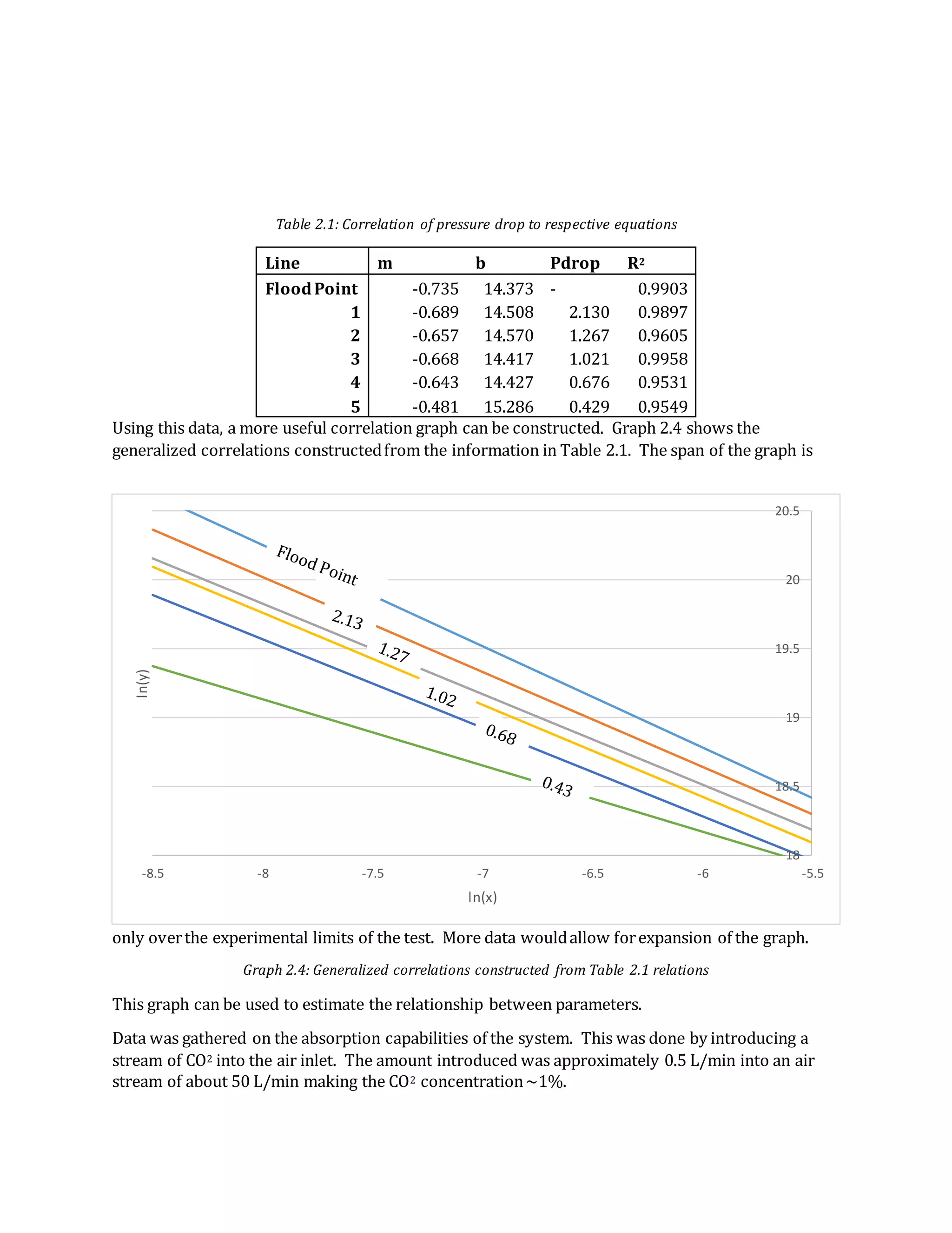
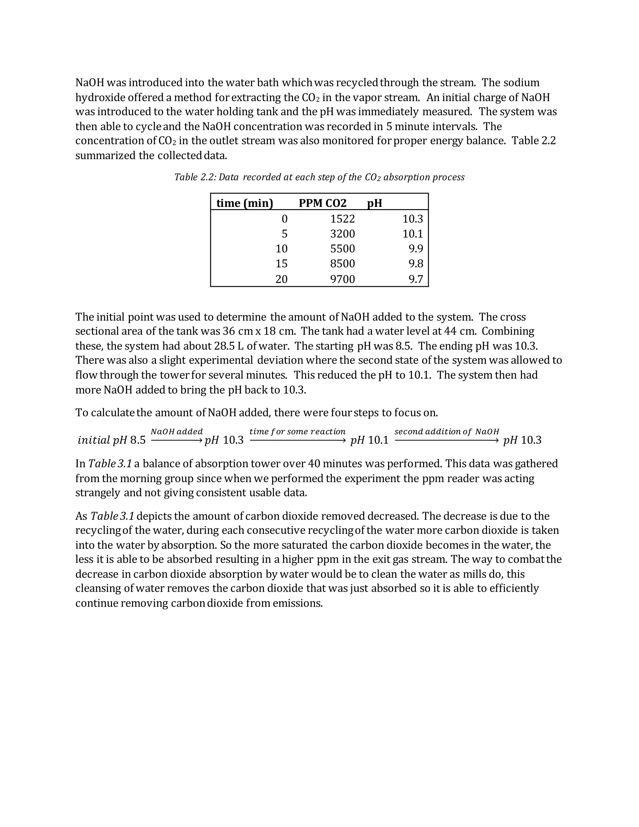
- The document summarizes an experiment on absorption processes using a countercurrent gas-liquid absorption tower. - Key findings include developing relationships between liquid flow rate, vapor flow rate, and pressure drop. Generalized correlations were constructed from these relationships. - Absorption of CO2 from air into water was also studied. Data showed decreasing CO2 removal over time as the water became saturated.

1. Joseph W. Lehmann
On Absorption Practice, Methods and Theory: An Empirical Example
2015
Oxford, Ohio-Miami University Engineering Laboratories

2. Introduction
Absorption offersa way to transfer material from one fluid stream to another. This has many
important and useful applications. For example, in the petroleum industry, a mixture of two
petrochemical compounds may exist with a desire to separate these components. If a solvent is
introduced which is immiscible to one component, and the other is able to dissolve into it, this
provides a method of removing one component or components from the primary stream. This
specific type of process is seen in many other industries and one of the most common applications
of this principle is in a packed absorption tower.
There are normally twoprimary fluid streams in an absorption process. The stream containing the
component of interest whichis to be removed, and a stream which the component of interest is
transferred to. Any twoimmiscible fluids may participate in this. For the case of this experiment, it
is a countercurrent flow of gas and liquid fluids. This provides additional assistance due to the
drastic difference in density of the streams, aiding in the countercurrent interaction.
Absorption processes utilize a packing material whichis included in the absorption tower. This
packing material disturbs the flow of the fluids and increases the surface area exposure between
the fluids. In this experiment, rasching rings were used as the packing material. The surface area
per volumeof these rings is about 440 m2/m3.
This experiment’s goal is to study the effectsof absorption in a countercurrent gas-liquid phase
process. There will also be development to analyze and understand the characteristics of the
absorption tower.
Experimental Development
The first step in the experimental procedure was to develop an understanding of the toweritself.
The two fluids utilized were water and ambient air. The absorption towerhad a water inlet at the
top of the tower and an air inlet at the bottom of the towerwith gravity being the driving force for
the tower. There were twolocations where pressure within the tower was measured, one location
was 17 inches below the surface of the packing material, the second 50 inches. These two
measurements would be used to determine the pressure drop over the span between the pressure
readings.
An important measurement in absorption towermechanics is the floodpoint. The floodpoint is
defined as the point at which there is no consistent pressure drop reading. This is commonly
observed as a foaming within the absorption tower (and a rising liquid level in a vapor-liquid
absorption process). This is an unstable state in the system and should be avoided in industry.
To develop an understanding of the absorption tower, a relationship between liquid flowrate,vapor
flowrate,and pressure drop was developed. These relationships offereda way to graphically
interpret the effects of varying the flowrate of water with the flowrateof the vapor and how the
pressure change responds.
The common graphical representation relates the log of pressure drop to the air flowrate per flow
area. The units of the air flowrateare in lbm/s ft2. The air flowratein L/min is given. To convert
this to a useful value, the air density and cross sectional area must be used. At room temperature,

3. air density is approximately 1.184 kg/m3 or 0.001184 kg/L. The diameter of the circulartube is 80
mm or 0.2625 ft. This results in a cross sectional area of 0.0541 ft2.The equation used:
𝐺𝑦 = (
𝐴𝑖𝑟 𝐹𝑙𝑜𝑤𝑟𝑎𝑡𝑒 𝐿
𝑠
) (
0.001184 𝑘𝑔
𝐿
) (
2.205 𝑙𝑏
𝑘𝑔
) (
1
0.0514 𝑓𝑡2
) = 𝑀𝑎𝑠𝑠 𝐹𝑙𝑜𝑤𝑟𝑎𝑡𝑒 [
𝑙𝑏
𝑠 𝑓𝑡2
]
This is the same method to calculate the mass flow rate of water which has a density of 1 kg/L.
𝐺𝑥 = (
𝑊𝑎𝑡𝑒𝑟 𝐹𝑙𝑜𝑤𝑟𝑎𝑡𝑒 𝐿
𝑠
) (
1 𝑘𝑔
𝐿
) (
2.205 𝑙𝑏
𝑘𝑔
)(
1
0.0514 𝑓𝑡2
) = 𝑀𝑎𝑠𝑠 𝐹𝑙𝑜𝑤𝑟𝑎𝑡𝑒 [
𝑙𝑏
𝑠 𝑓𝑡2
]
Forming the first relationship, ln(Gy) willrepresent the x-axis of the graphical relationship. The y-
axis is the pressure drop on a logarithmic scale. This is calculated by:
𝑙𝑛 (
𝑃ℎ𝑖𝑔ℎ − 𝑃𝑙𝑜𝑤
∆𝐻
)
This is the difference in pressures divided by the distance between the reading points in the tower.
Creating a generalized correlation would require many data points relating the flow topressure
drop. From the worksheet, there were twoequations identified to represent the x and y axes for
constructing the generalized correlations. They are as follows.
𝑥 − 𝑎𝑥𝑖𝑠:
𝐺𝑥
𝐺𝑦
√
𝜌𝑦
𝜌𝑥
𝑦 − 𝑎𝑥𝑖𝑠:
𝐺𝑦
2 𝐹𝑝 (
62.3
𝜌𝑥
) 𝜇 𝑥
0.2
𝑔 𝑐 𝜌𝑥 𝜌𝑦
Where
𝐹𝑝 − 𝐹𝑙𝑜𝑜𝑑 𝑃𝑜𝑖𝑛𝑡 (= 1024 𝑓𝑡−1)
𝑔 𝑐 − 𝑝𝑟𝑜𝑝𝑜𝑟𝑡𝑖𝑜𝑛𝑎𝑙𝑖𝑡𝑦 𝑓𝑎𝑐𝑡𝑜𝑟 (= 32.174
𝑓𝑡 𝑙𝑏
𝑙𝑏𝑓 𝑠2
)
𝜇 𝑥 − 𝐿𝑖𝑞𝑢𝑖𝑥 𝑣𝑖𝑠𝑐𝑜𝑠𝑖𝑡𝑦 (8.90𝐸 − 4
𝑘𝑔
𝑠 𝑚
)
The relationship between these twoparameters wouldform the generalized correlation.

4. Results and Discussion
Graph 2.1 shows the relationship between the gas flowrateand pressure drop.
Graph 2.1: Pressure drop per length vs. air mass flowrate on a logarithmic scale
Graph 2.1 shows a rough correlation between the twovariables forall tests. The expectations were
for a roughly linear plot foreach data set whichis observed. Some lines do intersect whichis not as
expected, howeverthis is possibly due to measurement errors in the graph.
The flood point line seems to be almost linear. It may prove to be completely straight, howevernot
enough data was collectedto determine if this is true or not. The line resides at approximately -2.6
on the y-axis whichtranslates to a pressure drop of about 0.00243 Paper meter of packing
material. This couldbe used to predict a flood point during future analysis.
Graph 2.2: Basis for generalized correlation
-4.8
-4.3
-3.8
-3.3
-2.8
-2.3
5 5.2 5.4 5.6 5.8 6
log((pa-pb)/L)
log(Gy)
Water 0L/min
Water 1L/min
Water 2L/min
Water 3L/min
Water 4L/min
Linear (Flood Point)
17.5
18
18.5
19
19.5
20
20.5
-8.5 -8 -7.5 -7 -6.5 -6 -5.5
ln(y)
ln(X)
Water 1L/min
Water 2L/min
Water 3L/min
Water 4L/min

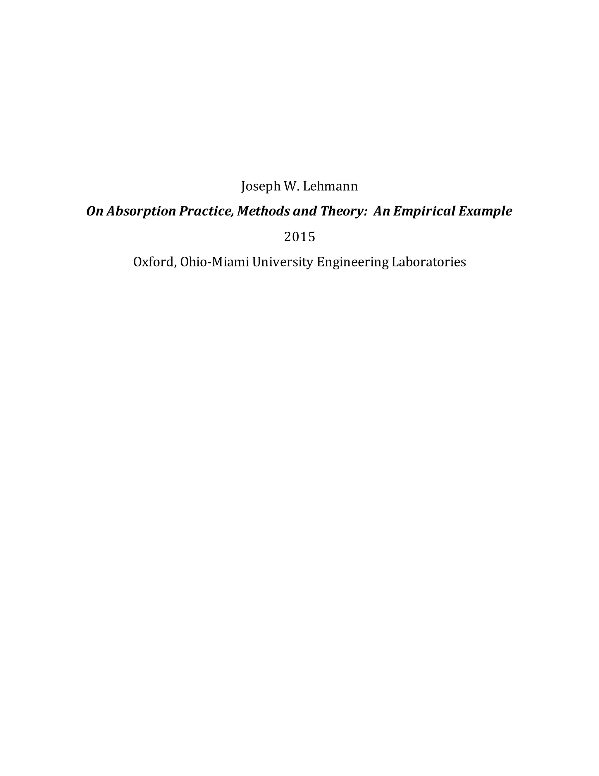
5. To constructthe generalized correlation, a graph of the data points was generated at first. This is
shown as Graph 2.2 with each data set corresponding to a different water flowrate. The axes are
described in the experimental development section and willbe restated.
𝑥 − 𝑎𝑥𝑖𝑠:
𝐺𝑥
𝐺𝑦
√
𝜌𝑦
𝜌𝑥
𝑦 − 𝑎𝑥𝑖𝑠:
𝐺𝑦
2 𝐹𝑝 (
62.3
𝜌𝑥
) 𝜇 𝑥
0.2
𝑔 𝑐 𝜌𝑥 𝜌𝑦
Eachpoint represents a different pressure drop relation. Again, the pressure drop is calculated
with respect to the total height difference. The units are also important as well.
𝑃𝑟𝑒𝑠𝑠𝑢𝑟𝑒 𝐷𝑟𝑜𝑝 =
𝑃ℎ𝑖𝑔ℎ − 𝑃𝑙𝑜𝑤
ℎ𝑒𝑖𝑔ℎ𝑡
[
𝑖𝑛 𝐻2 𝑂
𝑓𝑡
]
To constructthe correlation, points with similar pressure drops werefocused on and assessed for
the accuracy of the regression. This is shown in Graph 2.3.
Graph 2.3: Linear regression of pressure drops. See Table 2.1 for the parameters of each line moving from the
top line downward.
These regressions were significantly accurate and provided a basis forthe graphical construction.
The R2 values were all above 0.95 confirming the accuracy of the measurements. The linear
regression was accurateenough to remain the desired correlation method (as opposed to
exponential or other). The results are shown in Table 2.1 withthe slope of each line, the intercept,
the pressure drop value corresponding to the line, and the R2 value. The table is ordered so that
each column position relates to the position of each line in the graph, highest being first, lowest
being last. For example, the “floodpoint” line is the uppermost line on the graph. “Line 5” is the
lowermost line on the graph.
17.5
18
18.5
19
19.5
20
20.5
-9 -8.5 -8 -7.5 -7 -6.5 -6 -5.5
ln(y)
ln(x)

6. Table 2.1: Correlation of pressure drop to respective equations
Line m b Pdrop R2
FloodPoint -0.735 14.373 - 0.9903
1 -0.689 14.508 2.130 0.9897
2 -0.657 14.570 1.267 0.9605
3 -0.668 14.417 1.021 0.9958
4 -0.643 14.427 0.676 0.9531
5 -0.481 15.286 0.429 0.9549
Using this data, a more useful correlation graph can be constructed. Graph 2.4 shows the
generalized correlations constructedfrom the information in Table 2.1. The span of the graph is
only overthe experimental limits of the test. More data wouldallow forexpansion of the graph.
Graph 2.4: Generalized correlations constructed from Table 2.1 relations
This graph can be used to estimate the relationship between parameters.
Data was gathered on the absorption capabilities of the system. This was done by introducing a
stream of CO2 into the air inlet. The amount introduced was approximately 0.5 L/min into an air
stream of about 50 L/min making the CO2 concentration~1%.
18
18.5
19
19.5
20
20.5
-8.5 -8 -7.5 -7 -6.5 -6 -5.5
ln(y)
ln(x)

7. NaOH was introduced into the water bath whichwas recycledthrough the stream. The sodium
hydroxide offered a method forextracting the CO2 in the vapor stream. An initial charge of NaOH
was introduced to the water holding tank and the pH was immediately measured. The system was
then able to cycleand the NaOH concentration was recorded in 5 minute intervals. The
concentration of CO2 in the outlet stream was also monitored forproper energy balance. Table 2.2
summarized the collecteddata.
Table 2.2: Data recorded at each step of the CO2 absorption process
time (min) PPM CO2 pH
0 1522 10.3
5 3200 10.1
10 5500 9.9
15 8500 9.8
20 9700 9.7
The initial point was used to determine the amount of NaOH added to the system. The cross
sectional area of the tank was 36 cm x 18 cm. The tank had a water level at 44 cm. Combining
these, the system had about 28.5 L of water. The starting pH was 8.5. The ending pH was 10.3.
There was also a slight experimental deviation where the second state of the system was allowed to
flow through the towerfor several minutes. This reduced the pH to 10.1. The system then had
more NaOH added to bring the pH back to 10.3.
To calculatethe amount of NaOH added, there were foursteps to focus on.
𝑖𝑛𝑖𝑡𝑖𝑎𝑙 𝑝𝐻 8.5
𝑁𝑎𝑂𝐻 𝑎𝑑𝑑𝑒𝑑
→ 𝑝𝐻 10.3
𝑡𝑖𝑚𝑒 𝑓𝑜𝑟 𝑠𝑜𝑚𝑒 𝑟𝑒𝑎𝑐𝑡𝑖 𝑜 𝑛
→ 𝑝𝐻 10.1
𝑠𝑒𝑐𝑜𝑛𝑑 𝑎𝑑𝑑𝑖𝑡𝑖 𝑜 𝑛 𝑜𝑓 𝑁𝑎𝑂𝐻
→ 𝑝𝐻 10.3
In Table3.1 a balance of absorption tower over 40 minutes was performed. This data was gathered
from the morning group since when we performed the experiment the ppm reader was acting
strangely and not giving consistent usable data.
As Table3.1 depicts the amount of carbon dioxide removed decreased. The decrease is due to the
recyclingof the water, during each consecutive recyclingof the water more carbon dioxide is taken
into the water by absorption. So the more saturated the carbon dioxide becomes in the water, the
less it is able to be absorbed resulting in a higher ppm in the exit gas stream. The way to combatthe
decrease in carbon dioxide absorption by water would be to clean the water as mills do, this
cleansing of water removes the carbon dioxide that was just absorbed so it is able to efficiently
continue removing carbondioxide from emissions.

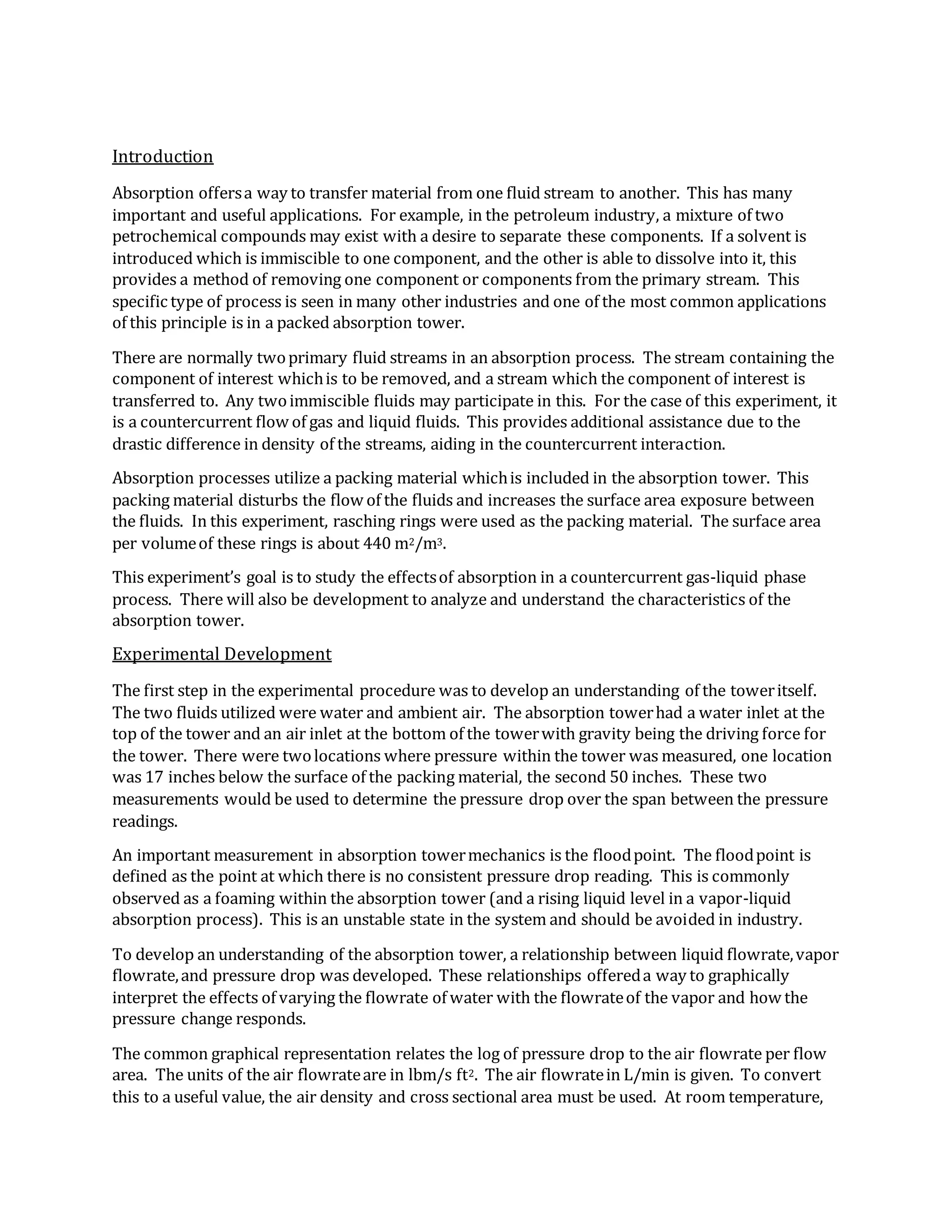
8. Table 3.1: ppm Balance of the absorption tower
In Table3.2 a very similar balance is done but instead of ppm the numbers have been converted
into moles of carbon dioxide in water.Similar explanations and ideas revolvearound this table as
they do for the discussion of Table3.1. Using this table we can determine that roughly 0.035 moles
of carbon dioxide are now in the water.
Table 3.2: mole balance of the Absorption Tower
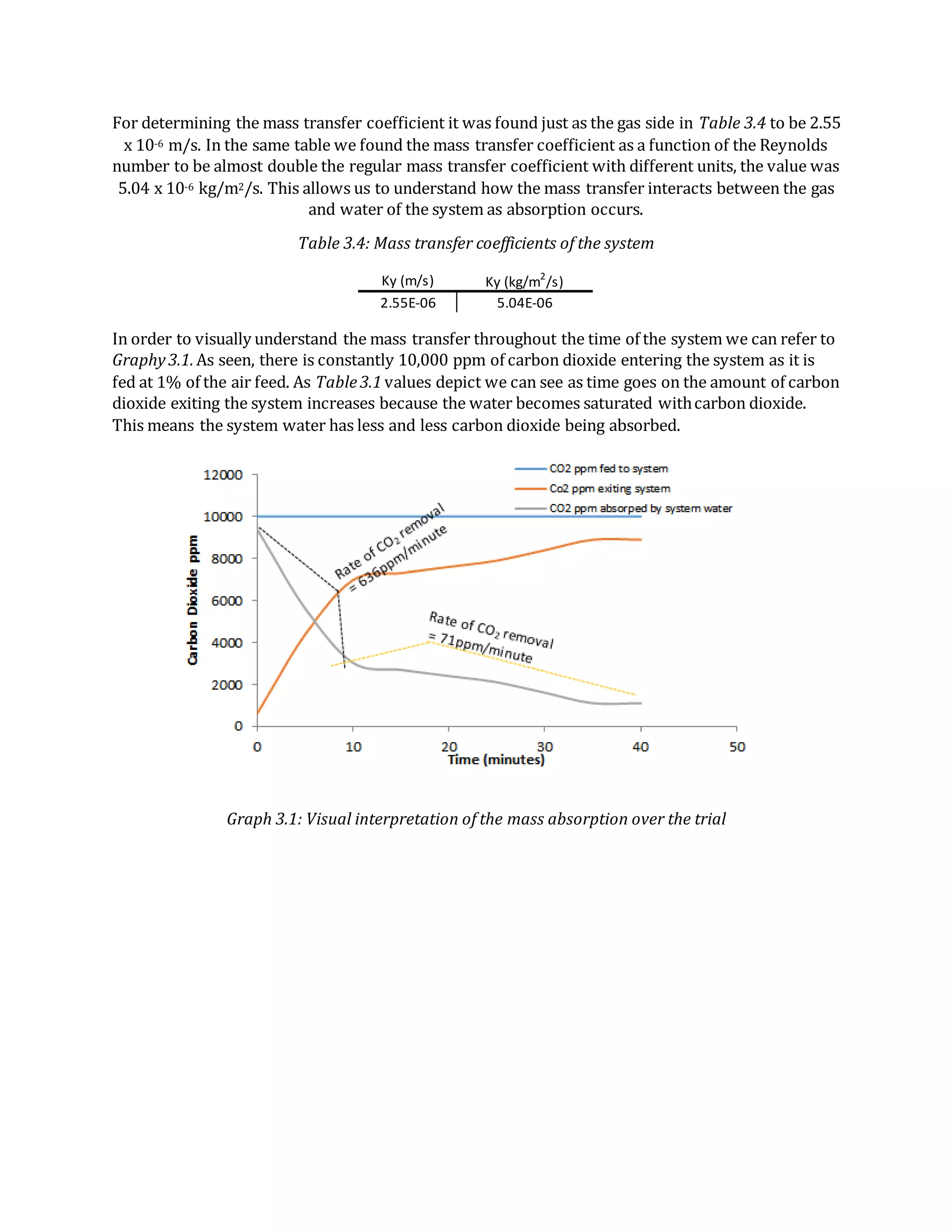
Here in Table3.3 we can observe how the rate of carbon dioxide removal from the gas phase by
absorption in water changes throughout the experiment. For the first ten minutes the rate of
removal was very high and efficientat around 640 ppm/min of carbonremoved fromgas phase.
After ten minutes the water became toosaturated and the rate of removal dropped to 71 ppm/min.
The last removal rate that we lookedat is the bold number whichdetermines the rate over the
entire forty minute period, we found that the overall rate of carbon dioxide removal from the gas
phase by absorption by water was 207 ppm/min.
Table 3.3: Rate of Removal of Carbon Dioxide
Time (min) pH (z)
CO2 ppm fed to
system
Co2 ppm exiting
system
CO2 ppm
absorped by
system water
0 10.5 10000 617 9383
5 10.5 10000 4381 5619
10 10.1 10000 6980 3020
15 10.1 10000 7310 2690
20 9.9 10000 7600 2400
25 9.8 10000 7900 2100
30 9.7 10000 8400 1600
35 9.7 10000 8900 1100
40 9.5 10000 8900 1100
Time (min) pH (z) Exit CO2 mol frac Exit CO2 moles/min [H+] ions Ct (moles/L)
Moles
CO2 in
water
CO2
Moles
leaving
0 10.5 0.0006 0.0013 3.16E-11 -1.14E-06 0.0000 0.0000
5 10.5 0.0044 0.0090 3.16E-11 -1.14E-06 0.0000 0.0448
10 10.1 0.0070 0.0143 7.94E-11 1.10E-04 0.0031 0.1429
15 10.1 0.0073 0.0150 7.94E-11 1.10E-04 0.0031 0.2244
20 9.9 0.0076 0.0156 1.26E-10 1.62E-04 0.0046 0.3111
25 9.8 0.0079 0.0162 1.58E-10 1.85E-04 0.0053 0.4043
30 9.7 0.0084 0.0172 2.00E-10 2.05E-04 0.0059 0.5158
35 9.7 0.0089 0.0182 2.00E-10 2.05E-04 0.0059 0.6376
40 9.5 0.0089 0.0182 3.16E-10 2.39E-04 0.0068 0.7287
Time
Range
(min)
Rate of
Removal
(ppm/min)
0 - 10 636
10 - 40 71
0 - 40 207

9. For determining the mass transfer coefficient it was found just as the gas side in Table 3.4 to be 2.55
x 10-6 m/s. In the same table we found the mass transfer coefficient as a function of the Reynolds
number to be almost double the regular mass transfer coefficient with different units, the value was
5.04 x 10-6 kg/m2/s. This allows us to understand how the mass transfer interacts between the gas
and water of the system as absorption occurs.
Table 3.4: Mass transfer coefficients of the system
In order to visually understand the mass transfer throughout the time of the system we can refer to
Graphy3.1.As seen, there is constantly 10,000 ppm of carbon dioxide entering the system as it is
fed at 1% of the air feed. As Table3.1 values depict we can see as time goes on the amount of carbon
dioxide exiting the system increases because the water becomes saturated withcarbon dioxide.
This means the system water has less and less carbon dioxide being absorbed.
Graph 3.1: Visual interpretation of the mass absorption over the trial
Ky (m/s) Ky (kg/m2
/s)
2.55E-06 5.04E-06

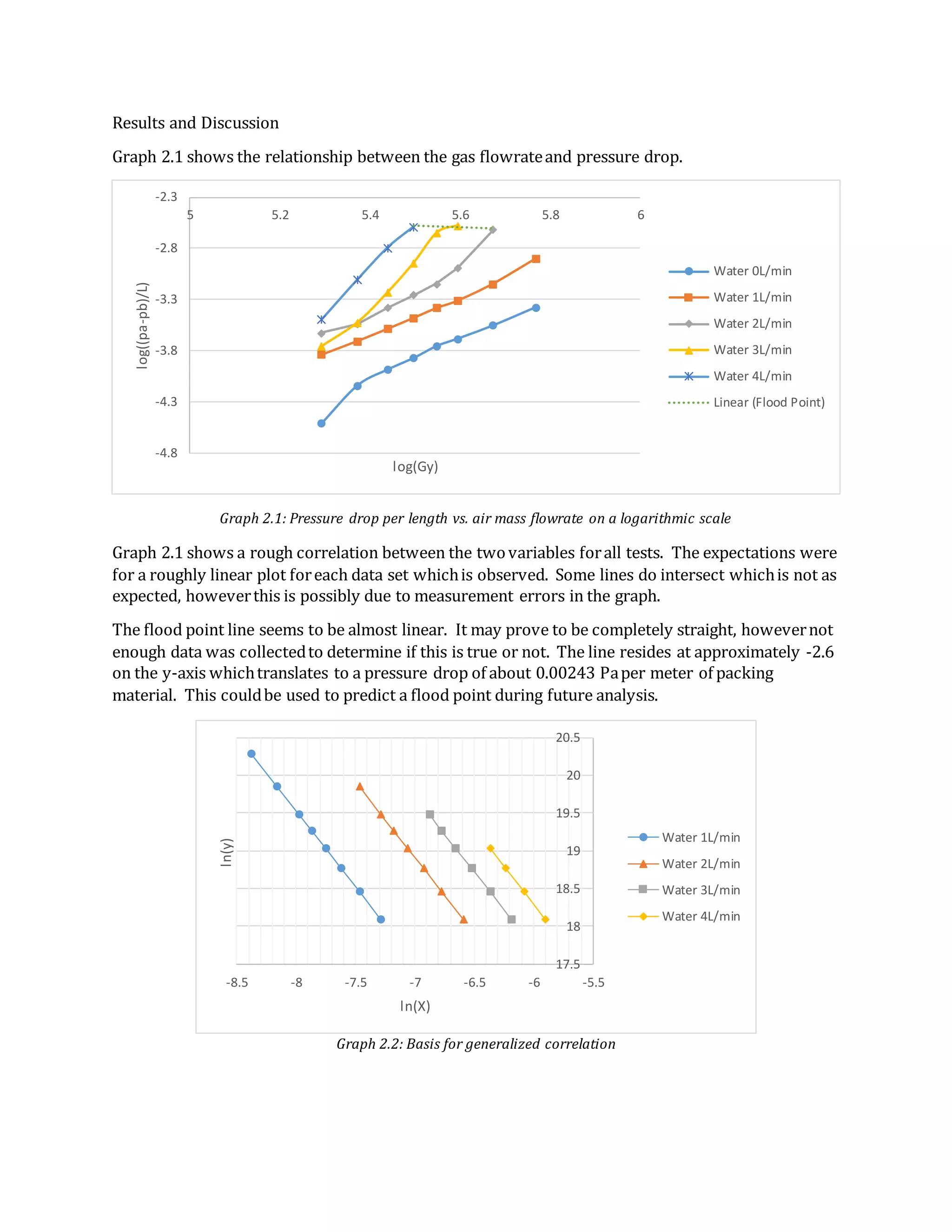
10. Table 4: Tabulation of back calculated values for the addition on NaOH to raise pH from 8.3
to 10.3
Additional Notes and Further Inquiry:
The back calculationof the mass of NaOH needed to be added to our system to raise the pH
by three points was rather straightforward. It also yielded results that were pretty close to the
actual, known value of NaOH added to the system. The principal behind this calculation was that pH
is based off of molarity, whichis a concentration measurement. The pH gave us a moles/liter value.
As shown above,we calculated these values. From there, we knew that there was about 28.5 liters
of water solution in out system. This allowed us to multiply the difference in molarities by the
amount of liters of solution. The stoichiometry of NaOH and H2O is one to one, so a direct molar
correlation could be achieved. This yielded a molar value forNaOH. From there, the molecular
weight was used to yield a final mass value, of about 4.4 grams of NaOH. As noted before, we knew
the amount of NaOH that we added, because we weighed it before the addition. Our measured
weight was about 4.1 grams. This value is very closeto the theoretically calculated value. Some
reasons why it coulddiffer slightly are that while the waterwas flowing,residual acidic media may
have been left overon the walls and parts of the system. Also, human error in calculation probably
played a role in the discrepancy. Overall,we were not very surprised by this calculation and
expected a small error involved.
Please Inquire at lehmanjw@miamioh.edu
Back Calculated Parameters Calculated Value
Molarity of Solution at pH of 8.3 [H+] 5.013 x 10-9 moles/liter
Molarity of Solution at pH of 10.3 [H+] 5.001 x 10-11 moles/liter
Moles of NaOH needed to be added 0.110 moles NaOH
Weight of NaOH to be added (39.9 g/mol) 4.412 grams NaOH