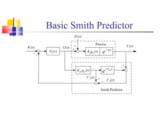
This document discusses dead-time compensation techniques for processes with time delays. It introduces the Smith predictor method for dead-time compensation and compares its performance to a conventional PID controller. An improved Smith predictor is also presented which incorporates a prediction error filter to better handle models that are not completely accurate. Simulation examples are provided comparing the different control techniques on processes with varying time delays.

1. Dead-Time Compensation
(纯滞后补偿)
Lei Xie
Institute of Industrial Control,
Zhejiang University, Hangzhou, P. R.
China

2. Contents
 Introduction
 Smith Predictor for Dead-Time
Compensation
 Improved Smith Predictor
 Simulation Examples
 Summary

3. Problem Discussion
(1) For the controlled processes, configure your
Simulink model & compare their results.
(2) Can you provide some compensation approaches
for processes with variable & notable dead-time ?
Process
G ( s ) 2.0 e
-
2s
Models: ;
p ( ) 2.0 8s
p e
G s -
= .
s
+
4 1
s
+
4 1
=

4. Conventional PID Control Systems
Process
G ( s ) 2.0 e
-
2s
Models: ;
p ( ) 2.0 8s
p e
G s -
= .
s
+
4 1
s
+
4 1
=
Question：Use Ziegler-Nichols or Lambda tuning method to obtain
PID parameters and compare their values.
Please see the SimuLink model …SISODelayPlant / PIDLoop.mdl

5. Simulation Example #1
0 20 40 60 80 100 120 140 160 180 200
78
76
74
72
70
68
66
64
62
60
58
Output of Transmitter
Time, min
%
setpoint
Ziegler-Nichols Tuning
Lambda Tuning
;
( ) 2.0 2s
p e
G s -
s
+
4 1
=
For PID Controller,
Z-N tuning: Kc = 1.2,
Ti = 4 min, Td = 1 min
Lambda tuning:
Kc = 0.83, Ti = 4 min ,
Td = 1 min

6. Simulation Example #2
0 20 40 60 80 100 120 140 160 180 200
80
78
76
74
72
70
68
66
64
62
60
58
Time, min
%
Output of Transmitter
set point
Z-N tuning
Lambda tuning, Td = 1 min
Lambda tuning, Td = 4 min
( ) = 2.0 -
8 ;
p G s e
s
+
4 1
s
For PID Controller,
Z-N tuning: Kc = 0.3,
Ti = 16 min, Td = 4 min
Lambda tuning:
Kc = 0.2, Ti = 4 min ,
Td = 1 min

7. Smith’s Idea (1957)
D (s)
+
Process
R (s) Y (s)
Gc(s) +
Kpgp (s) + _
e-t s
D (s)
+
Process
R (s) Y (s)
Gc(s) +
Kpgp (s) + _
e-t s

8. Basic Smith Predictor
D (s)
Process
R (s) +
Y (s)
Gc(s) +
Kpgp (s) + _
e-t s
U(s)
Km gm (s) s e-t m
+ _
Y 2(s)
Smith Predictor
Y 1(s) +
+

9. Smith Predictor #2
+ _
+
Gc(s) +
D (s)
R (s) Y (s)
+
_
U (s) s
K g s e p -t ( )
p p
K g (s) m m
+
+
s
K g (s)e-t m
m m
Please see the SimuLink model …SISODelayPlant / PID_Smith.mdl

10. Results of Basic Smith Predictor
with an Accurate Model
0 20 40 60 80 100 120 140 160 180 200
80
78
76
74
72
70
68
66
64
62
60
58
Time, min
%
Output of Transmitter
set point
PID with Smith compensator
Simple PID
G s G s
=
=
m p
2.0 -
8
;
4 1
( ) ( )
s
e
s
+
Simple PID:
Kc = 0.2, Ti = 4 min ,
Td = 1 min
PID + Smith:
Kc = 2, Ti = 4 min ,
Td = 1 min

11. Results of Basic Smith Predictor
with an Inaccurate Model
0 20 40 60 80 100 120 140 160 180 200
85
80
75
70
65
60
55
Time, min
%
Output of Transmitter
set point
PID + Smith
Simple PID
( ) 2.0 -
8
;
-
6
G s e
s
+
4 1
=
( ) 2.0
G s e
s
+
4 1
s
m
s
p
=
Simple PID:
Kc = 0.2, Ti = 4 min ,
Td = 1 min
PID + Smith:
Kc = 2, Ti = 4 min ,
Td = 1 min

12. Improved Smith Predictor
+ _
+
Gc(s) +
D (s)
R (s) Y (s)
+
_
U (s) s
K g s e p -t ( )
p p
K g (s) m m
+
+
s
K g (s)e-t m
m m
Gf(s)
1
( ) 1
+
=
T s
G s
f
Prediction Error Filter ： f

13. Results of Improved Smith
Predictor with an Inaccurate Model
0 20 40 60 80 100 120 140 160 180 200
80
78
76
74
72
70
68
66
64
62
60
58
Time, min
%
Output of Transmitter
set point
PID + Smith with Gm =Gp
PID + Smith with Gm <> Gp
Simple PID
( ) 2.0 -
8
s
;
G s e
s
=
+
( ) 2.0 -
6
;
4 1
G s e
s
+
4 1
=
( ) 1
s
+
4 1
m
s
p
G s
f
=
PID + Smith:
Kc = 2, Ti = 4 min ,
Td = 1 min

14. Summary
 The principle of Smith predictor for dead-time
compensation
 Improved Smith predictor for a controlled
process with an inaccurate model
 Comparison of the Simple PID and the PID
with a Smith predictor

15. Next Topic: Coupling of Multivariable
Systems and Decoupling
 Concept of Relative Gains
 Calculation of Relative Gain Matrix
 Rule of CVs and MVs Pairing
 Linear Decoupler from Block Diagrams
 Nonlinear Decoupler from Basic Principles
 Application Examples

16. Problem Discussion
for Next Topic
For the two-input-two-input
controlled system, design
your control schemes.
Suppose that
F = F + F C = C F +
C F
, 1 1 2 2
;
1 2 F +
F
1 2
;
F 0.5 5
s
m m
2 1
,
C
, 1
1
4 1
+
=
+
=
+
=
-
s
e
A
C
C s
F s
Initial states:
F 0
= F 0
= C = C =
1 2
75, 25, 60%, 40%. 1 2