This document discusses arrays of radiating elements and how to shape their radiation patterns. It begins by explaining that arrays can provide more directive characteristics than single elements by combining the fields from multiple elements constructively in desired directions and destructively elsewhere. The key controls for shaping an array's pattern are its geometry, element spacing, excitation amplitudes, excitation phases, and individual element patterns. It then provides examples of calculating the radiation pattern for a two-element array and a uniform linear array with any number of elements. Important concepts covered include the array factor, nulls and maxima, and how to configure arrays for broadside or end-fire maximum radiation.
![Arrays
Ranga Rodrigo
August 19, 2010
Lecture notes are fully based on Balanis [?]. Some diagrams and text are directly
from the books.
Contents
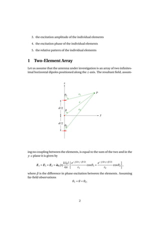
1 Two-Element Array 2
2 N-Element Linear Array: Uniform Amplitude and Spacing 6
Usually the radiation pattern of a single element is relatively wide, and each
element provides low values of directivity. In many applications it is necessary
to design antennas with very directive characteristics to meet the demands of
long distance communication. This can only be accomplished by increasing
the electrical size of the antenna. Enlarging the dimensions of single elements
often leads to more directive characteristics. Another way to enlarge the di-
mensions of the antenna, without necessarily increasing the size of the indi-
vidual elements, is to form an assembly of radiating elements in an electrical
and geometrical configuration. This new antenna, formed by multi-elements,
is referred to as an array. To provide very directive patterns, it is necessary that
the fields from the elements of the array interfere constructively (add) in the de-
sired directions and interfere destructively (cancel each other) in the remaining
space.
Shaping the Pattern of the Array
In an array of identical elements, there are usually five controls that can be
used to shape the overall pattern of the antenna. These are:
1. the geometrical configuration of the overall array (linear, circular, rectan-
gular, spherical, etc.)
2. the relative displacement between the elements
1](https://image.slidesharecdn.com/l06-230211162429-5f8d103c/85/Antenna-arrays-1-320.jpg)
![Arrays
Ranga Rodrigo
August 19, 2010
Lecture notes are fully based on Balanis [?]. Some diagrams and text are directly
from the books.
Contents
1 Two-Element Array 2
2 N-Element Linear Array: Uniform Amplitude and Spacing 6
Usually the radiation pattern of a single element is relatively wide, and each
element provides low values of directivity. In many applications it is necessary
to design antennas with very directive characteristics to meet the demands of
long distance communication. This can only be accomplished by increasing
the electrical size of the antenna. Enlarging the dimensions of single elements
often leads to more directive characteristics. Another way to enlarge the di-
mensions of the antenna, without necessarily increasing the size of the indi-
vidual elements, is to form an assembly of radiating elements in an electrical
and geometrical configuration. This new antenna, formed by multi-elements,
is referred to as an array. To provide very directive patterns, it is necessary that
the fields from the elements of the array interfere constructively (add) in the de-
sired directions and interfere destructively (cancel each other) in the remaining
space.
Shaping the Pattern of the Array
In an array of identical elements, there are usually five controls that can be
used to shape the overall pattern of the antenna. These are:
1. the geometrical configuration of the overall array (linear, circular, rectan-
gular, spherical, etc.)
2. the relative displacement between the elements
1](https://image.slidesharecdn.com/l06-230211162429-5f8d103c/75/Antenna-arrays-1-2048.jpg)
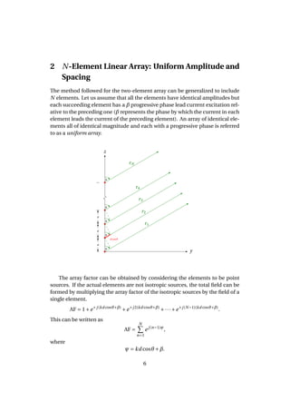
![Normalized,
AFn = cos
·
1
2
(kd cosθ +β)
¸
.
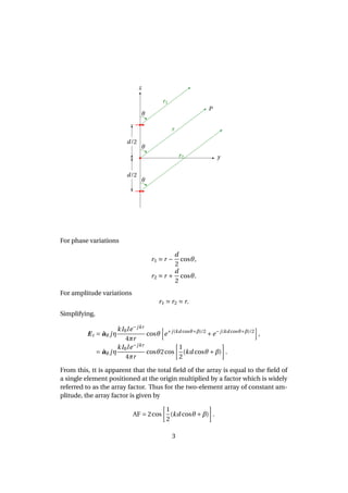
The array factor is a function of the geometry of the array and the excitation
phase. By varying the separation d and/or the phase β between the elements,
the characteristics of the array factor and of the total field of the array can be
controlled.
The far-zone field of a uniform two-element array of identical elements is
equal to the product of the field of a single element, at a selected reference point
(usually the origin), and the array factor of that array.
E(total) = [E(single element at reference point)]×[array factor].
This is valid for arrays with any number of identical elements which do not
necessarily have identical magnitudes, phases, and/or spacings between them.
The array factor, in general, is a function of the number of elements, their
geometrical arrangement, their relative magnitudes, their relative phases, and
their spacings. The array factor will be of simpler form if the elements have
identical amplitudes, phases, and spacings. Since the array factor does not de-
pend on the directional characteristics of the radiating elements themselves,
it can be formulated by replacing the actual elements with isotropic (point)
sources. Once the array factor has been derived using the point-source array,
the total field of the actual array is obtained by the use of the aforementioned
formula.
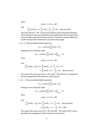
Example 1. Consider the two-element array of infinitesimal dipoles. Find the
nulls of the total field when d = λ/4 and
1. β = 0.
2. β = +π
2
.
3. β = −π
2 .
Solution:
1. β = 0 The normalized field is given by
Etn = cosθcos
³π
4
cosθ
´
Setting to zero to find the nulls,
Etn = cosθcos
³π
4
cosθ
´¯
¯
¯
θ=θn
= 0
4](https://image.slidesharecdn.com/l06-230211162429-5f8d103c/85/Antenna-arrays-4-320.jpg)
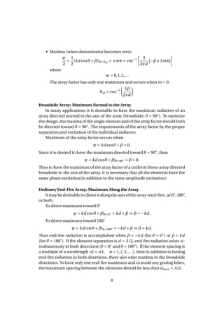
![AF = 1+e+jψ
+e+j2ψ
+···+e+j(N−1)ψ
,
AFe jψ
= e+jψ
+e+j2ψ
+e+j3ψ
+···+e+j Nψ
,
AF(e jψ
−1) = −1+e+j Nψ
.
AF =
·
e j Nψ
−1
e jψ −1
¸
,
= e j[(N−1)/2]ψ
·
e+j(N/2)ψ
−e−j(N/2)ψ
e+j(1/2)ψ −e−j(1/2)ψ
¸
,
= e j[(N−1)/2]ψ
"
sin
¡N
2
ψ
¢
sin
¡1
2ψ
¢
#
If the reference point is the physical center of the array
AF =
"
sin
¡N
2 ψ
¢
sin
¡1
2
ψ
¢
#
.
For small values of ψ,
AF '
"
sin
¡N
2 ψ
¢
1
2
ψ
#
.
As the maximum value is N, when normalized,
AFn =
1
N
"
sin
¡N
2
ψ
¢
sin
¡1
2ψ
¢
#
.
and
AFn '
1
N
"
sin
¡N
2 ψ
¢
N
2
ψ
#
.
Nulls and Maxima
• Nulls:
sin
µ
N
2
ψ
= 0 ⇒
N
2
ψ
¯
¯
¯
¯
θ=90◦
= ±nπ ⇒ θn = cos−1
·
λ
2πd
µ
−β±
2n
N
π
¶¸
,
where
n = 1,2,3,...
n 6= N,2N,3N,....
For n = N,2N,3N,..., correspond to maxima (sin(0)/0 form).
7](https://image.slidesharecdn.com/l06-230211162429-5f8d103c/85/Antenna-arrays-7-320.jpg)
![3_Antenna Array [Modlue 4] (1).pdf](https://cdn.slidesharecdn.com/ss_thumbnails/3antennaarraymodlue41-220419112111-thumbnail.jpg?width=640&height=640&fit=bounds)