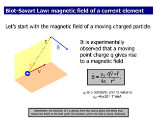
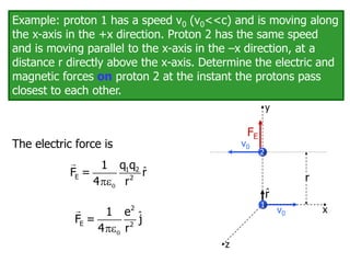
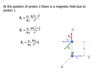
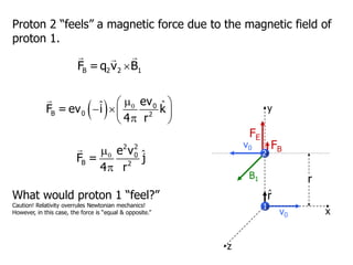
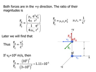
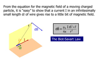
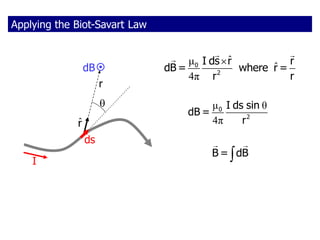
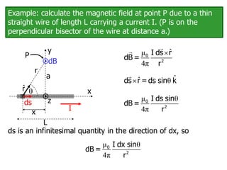
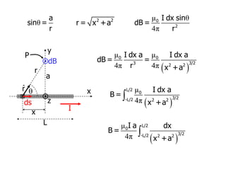
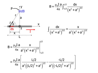
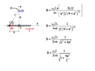
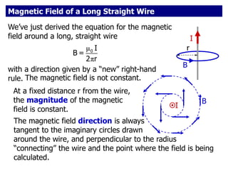
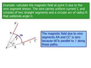
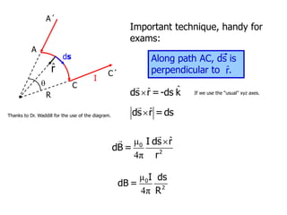
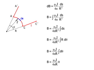
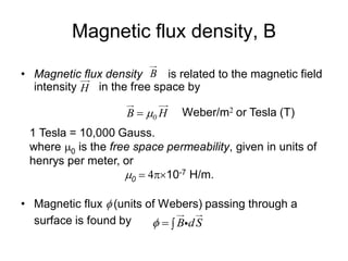
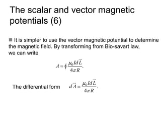
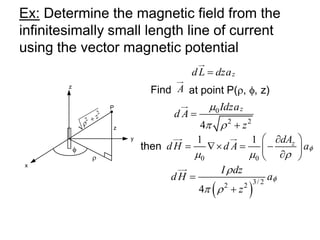
- The document discusses magnetic fields created by electric currents. It covers the magnetic field of a moving point charge, the Biot-Savart law for calculating the magnetic field from a current-carrying wire, and an example calculation of the magnetic field from a long straight wire.
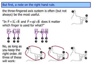
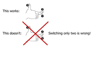
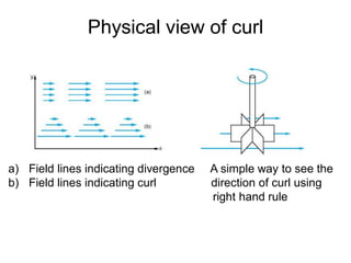
- The right hand rule is introduced for determining the direction of magnetic fields.
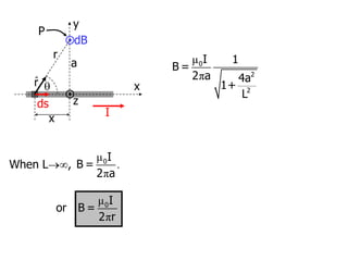
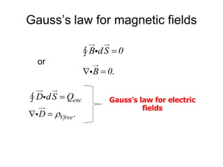
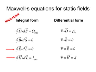
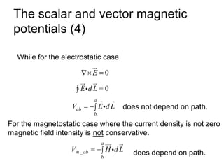
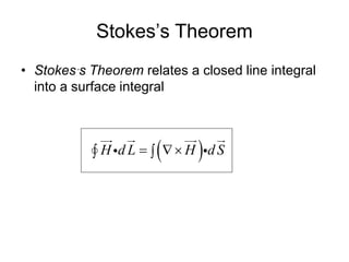
- Maxwell's equations for static magnetic fields in integral and differential form are presented.