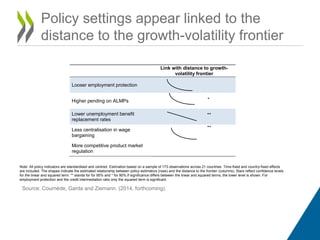
Download to read offline


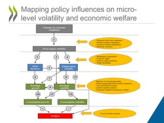
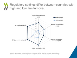
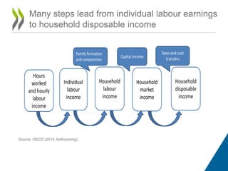
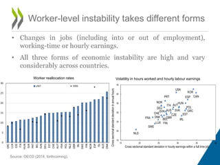
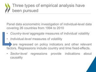
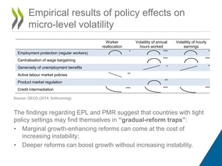
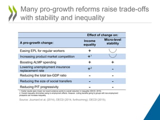
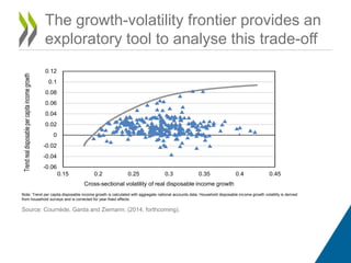

This document summarizes a seminar discussing the effects of growth-enhancing policies on microeconomic stability. It finds that while some pro-growth reforms can increase instability at the individual level, deeper reforms may boost growth without increasing volatility. Reforms like reducing employment protections and unemployment benefits can increase worker reallocation and earnings volatility, while well-designed social programs and competitive markets can attenuate these impacts. Policy settings are linked to a country's distance from the growth-volatility frontier, showing the importance of balancing economic goals.