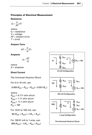
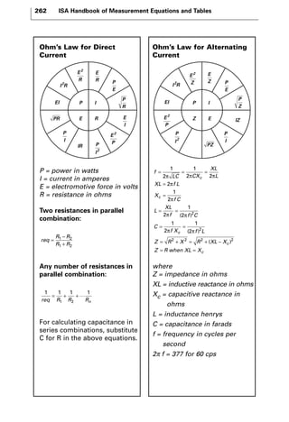
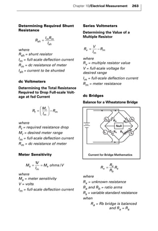
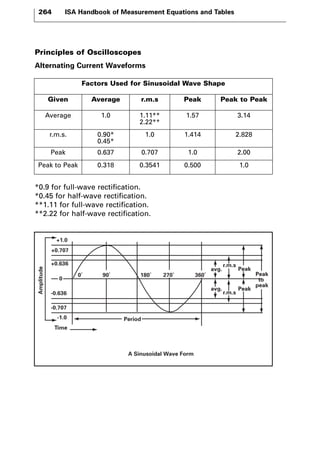
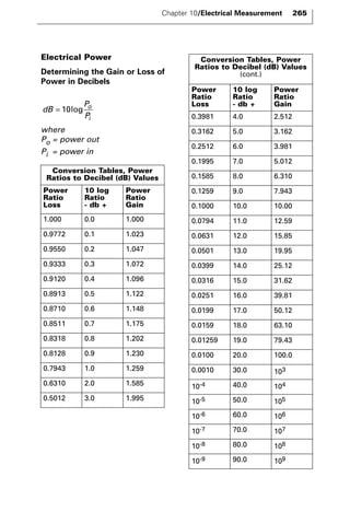
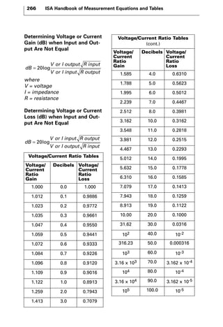
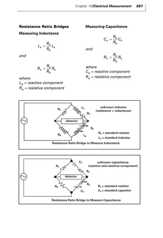
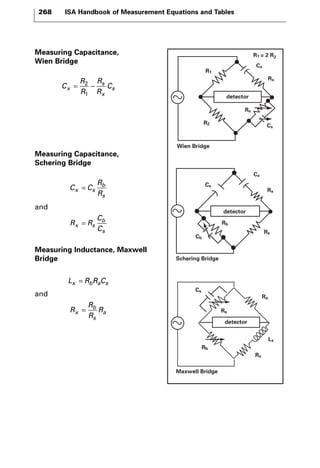
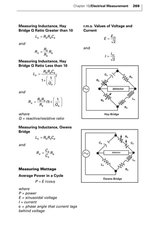
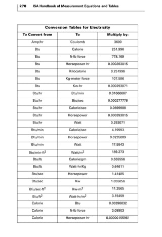
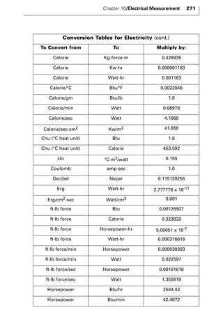
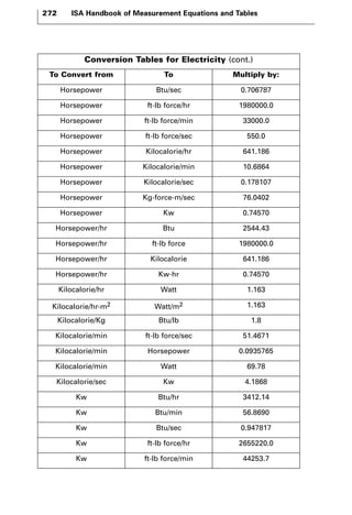
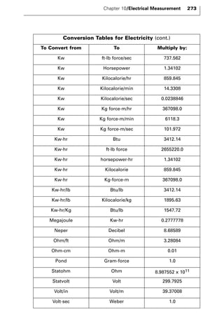
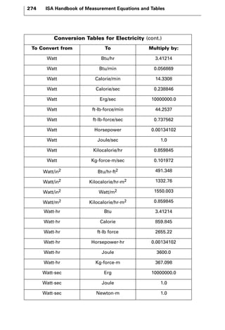
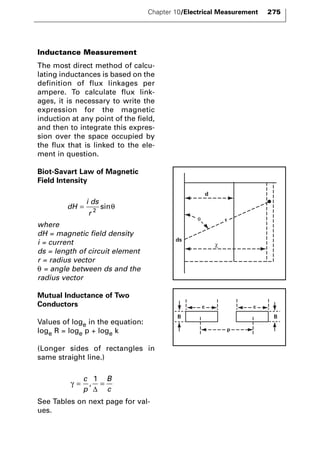
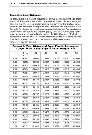
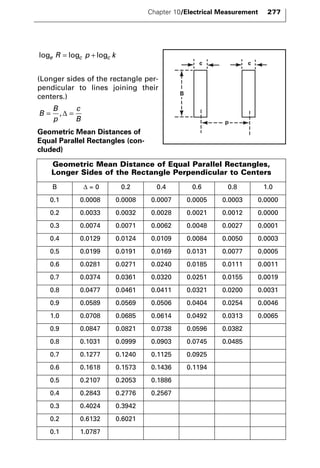
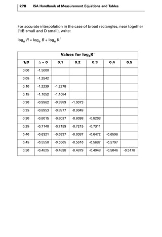
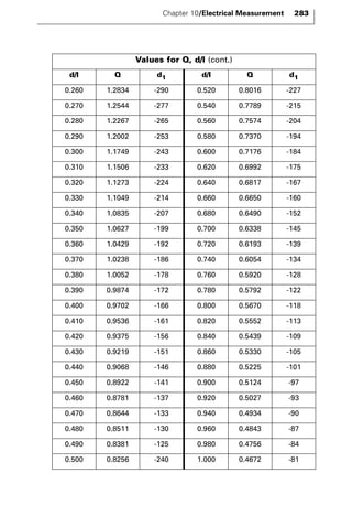
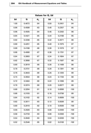
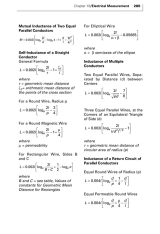
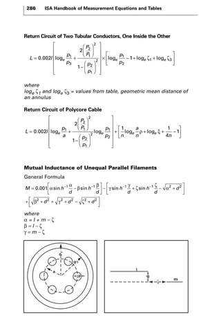
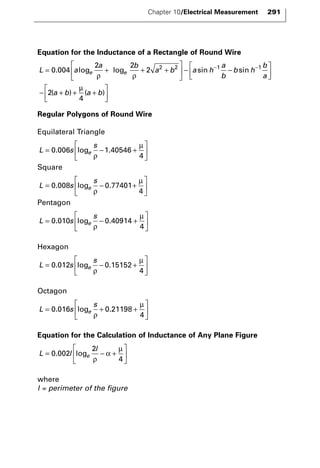
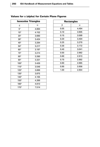
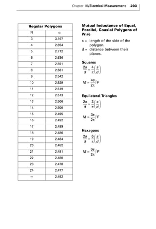
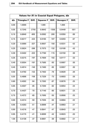
10 
Electrical Measurement 
Principles of Electrical Measurement. . . . . . . . . . . . . . . . . . . . . . . . 261 
Principles of Oscilloscopes . . . . . . . . . . . . . . . . . . . . . . . . . . . . . . . . 264 
Electrical Power . . . . . . . . . . . . . . . . . . . . . . . . . . . . . . . . . . . . . . . . . 265 
Voltage Ratios. . . . . . . . . . . . . . . . . . . . . . . . . . . . . . . . . . . . . . . . . . . 266 
Resistance Ratio Bridges. . . . . . . . . . . . . . . . . . . . . . . . . . . . . . . . . . 267 
Electricity Conversions . . . . . . . . . . . . . . . . . . . . . . . . . . . . . . . . . . . 270 
Inductance Measurement.. . . . . . . . . . . . . . . . . . . . . . . . . . . . . . . . . 275 
Geometric Mean Distances . . . . . . . . . . . . . . . . . . . . . . . . . . . . . . . . 276 
Values for Q . . . . . . . . . . . . . . . . . . . . . . . . . . . . . . . . . . . . . . . . . . . . 281 
Mutual Inductance . . . . . . . . . . . . . . . . . . . . . . . . . . . . . . . . . . . . . . . 285 
Self Inductance. . . . . . . . . . . . . . . . . . . . . . . . . . . . . . . . . . . . . . 285, 298
Principles of Electrical Measurement 
Resistance 
Ω = V 
AT 
T( ) 
where 
Ω = resistance 
V = voltage 
AT = ampere turns 
T = turns 
Ampere Turns 
Amperes 
AT 
A 
where 
A = amperes 
V 
= T 
Ω 
( ) 
AT = 
Ω 
Direct Current 
The Universal (Arytron) Shunt 
For 0 to 10 mA, use: 
0.009 (Rsh1 +Rsh2 +Rsh3) = 0.001(Rm) 
where 
Rsh1 = 0.111 ohm shunt 
Rsh2 = 1.11 ohm shunt 
Rsh3 = 11.1 ohm shunt 
Rm = 100 
For 10.01 to 100 mA, use: 
99 (Rsh2 +Rsh3) = 1(Rm +Rsh1) 
For 100.01 mA to 1 amp, use: 
999 (Rsh3) = 1(Rm +Rsh1 +Rsh2) 
Chapter 10/Electrical Measurement 261 
Rm = 100 
Rsh3 
M 
10 mA Configuration 
Rsh2 Rsh1 
Rm = 100 
Rsh2 
Rsh1 
Rm = 100 
9/ 
1/ 
Rsh1 
Rsh2 
99/ 1/ 
999/ 
Rsh3 
M 
100 mA Configuration 
1/ 
Rsh3 
M 
1 amp Configuration 
The Universal (Arytron) Shunt
262 ISA Handbook of Measurement Equations and Tables 
Ohm’s Law for Direct 
Current 
2 
EI EI 
2 
P = power in watts 
I = current in amperes 
E = electromotive force in volts 
R = resistance in ohms 
Two resistances in parallel 
combination: 
= − 
1 2 
1 2 
Any number of resistances in 
parallel combination: 
For calculating capacitance in 
series combinations, substitute 
C for R in the above equations. 
Ohm’s Law for Alternating 
Current 
f 
2 
1 
2 
1 
= = = 
= 
= 
π LC 2 π CX 
2 
π 
π 
XL 
L 
2 
2 
1 
2 
XL f L 
X 
f C 
L 
1 
2 
π 
XL 
f f C 
C 
= = 
π π 
1 
f X 
c 
c 
= 
2 
π 
2 
2 
( ) 
c 
1 
2 2 
( ) 
f L 
2 2 2 2 
Z R X R XL X 
Z RwhenXL X 
where 
Z = impedance in ohms 
XL = inductive reactance in ohms 
Xc = capacitive reactance in 
ohms 
L = inductance henrys 
C = capacitance in farads 
f = frequency in cycles per 
second 
2π f = 377 for 60 cps 
c 
c 
= 
= + = + − 
= = 
( ) 
π 
1 = 1 + 1 +1 
req R1 R2  
Rn 
req 
R R 
R R 
+ 
P 
E 
I 
R 
P 
Z 
I 
E 
IR 
IZ 
E 
R 
E 
P 
E 
P 
E 
Z 
E 
I 
E 
R 
E 
Z 
I R 2 I R 2 P 
E 
P 
E 
P 
I 2 
P 
I 2 
P 
I 
P 
I 
PR 
P 
R 
PZ 
P 
Z
Determining Required Shunt 
Resistance 
m m 
sh 
= 
where 
Rsh = shunt resistor 
Im = full-scale deflection current 
Rm = dc resistance of meter 
Ish = current to be shunted 
dc Voltmeters 
Determining the Total Resistance 
Required to Drop Full-scale Volt-age 
at fsd Current 
r 
m 
 
= m 
where 
Rt = required resistance drop 
Mr = desired meter range 
Im = full-scale deflection current 
Rm = dc resistance of meter 
Meter Sensitivity 
= = s 1 
where 
Ms = meter sensitivity 
V = volts 
Im = full-scale deflection current 
Series Voltmeters 
Determining the Value of a 
Multiple Resistor 
= − m 
where 
Rv = multiple resistor value 
V = full-scale voltage for 
desired range 
Im = full-scale deflection current 
Rm = meter resistance 
dc Bridges 
Balance for a Wheatstone Bridge 
Rb Ra 
lb 
lx ls 
a 
b 
Rx Rs 
la 
= s 
where 
Rx = unknown resistance 
Ra and Rb = ratio arms 
Rs = variable standard resistance 
when 
Ra = Rb bridge is balanced 
and Rx = Rs 
R 
R 
R 
x R 
R 
V 
I 
v R 
m 
M 
V 
I 
s M ohms V 
m 
/ 
R 
M 
I 
t R 
  
 
  
− 
R 
I R 
sh I 
Chapter 10/Electrical Measurement 263 
Null 
Current for Bridge Mathematics
264 ISA Handbook of Measurement Equations and Tables 
Principles of Oscilloscopes 
Alternating Current Waveforms 
Factors Used for Sinusoidal Wave Shape 
Given Average r.m.s Peak Peak to Peak 
Average 1.0 1.11** 
2.22** 
*0.9 for full-wave rectification. 
*0.45 for half-wave rectification. 
**1.11 for full-wave rectification. 
**2.22 for half-wave rectification. 
1.57 3.14 
r.m.s. 0.90* 
0.45* 
1.0 1.414 2.828 
Peak 0.637 0.707 1.0 2.00 
Peak to Peak 0.318 0.3541 0.500 1.0 
+1.0 
+0.707 
+0.636 
0 
-0.636 
-0.707 
-1.0 
Time 
Amplitude 
0° 90° 180° 270° 360° 
Period 
avg. 
avg. 
r.m.s 
r.m.s 
Peak 
Peak 
Peak 
to 
peak 
A Sinusoidal Wave Form
Electrical Power 
Determining the Gain or Loss of 
Power in Decibels 
dB 
P 
P 
o 
i 
= 10log 
where 
Po = power out 
Pi = power in 
Conversion Tables, Power 
Ratios to Decibel (dB) Values 
(cont.) 
Power 
Ratio 
Loss 
10 log 
Ratio 
- db + 
Power 
Ratio 
Gain 
0.3981 4.0 2.512 
0.3162 5.0 3.162 
0.2512 6.0 3.981 
0.1995 7.0 5.012 
0.1585 8.0 6.310 
0.1259 9.0 7.943 
0.1000 10.0 10.00 
0.0794 11.0 12.59 
0.0631 12.0 15.85 
0.0501 13.0 19.95 
0.0399 14.0 25.12 
0.0316 15.0 31.62 
0.0251 16.0 39.81 
0.0199 17.0 50.12 
0.0159 18.0 63.10 
0.01259 19.0 79.43 
0.0100 20.0 100.0 
0.0010 30.0 103 
10-4 40.0 104 
10-5 50.0 105 
10-6 60.0 106 
10-7 70.0 107 
10-8 80.0 108 
10-9 90.0 109 
Conversion Tables, Power 
Ratios to Decibel (dB) Values 
Power 
10 log 
Power 
Ratio 
Ratio 
Ratio 
Loss 
- db + 
Gain 
1.000 0.0 1.000 
0.9772 0.1 1.023 
0.9550 0.2 1.047 
0.9333 0.3 1.072 
0.9120 0.4 1.096 
0.8913 0.5 1.122 
0.8710 0.6 1.148 
0.8511 0.7 1.175 
0.8318 0.8 1.202 
0.8128 0.9 1.230 
0.7943 1.0 1.259 
0.6310 2.0 1.585 
0.5012 3.0 1.995 
Chapter 10/Electrical Measurement 265
266 ISA Handbook of Measurement Equations and Tables 
Determining Voltage or Current 
Gain (dB) when Input and Out-put 
Are Not Equal 
where 
V = voltage 
I = impedance 
R = resistance 
Determining Voltage or Current 
Loss (dB) when Input and Out-put 
Are Not Equal 
dB 
V or I input R output 
V or I output R input 
= 20log 
dB 
V or I output R input 
V or I input R output 
= 20log 
Voltage/Current Ratio Tables 
(cont.) 
Voltage/ 
Current 
Ratio 
Gain 
Decibels Voltage/ 
Current 
Ratio 
Loss 
1.585 4.0 0.6310 
1.788 5.0 0.5623 
1.995 6.0 0.5012 
2.239 7.0 0.4467 
2.512 8.0 0.3981 
3.162 10.0 0.3162 
3.548 11.0 0.2818 
3.981 12.0 0.2515 
4.467 13.0 0.2293 
5.012 14.0 0.1995 
5.632 15.0 0.1778 
6.310 16.0 0.1585 
7.079 17.0 0.1413 
7.943 18.0 0.1259 
8.913 19.0 0.1122 
10.00 20.0 0.1000 
31.62 30.0 0.0316 
102 40.0 10-2 
316.23 50.0 0.000316 
103 60.0 10-3 
3.16 x 10³ 70.0 3.162 x 10⁻⁴ 
104 80.0 10-4 
3.16 x 10⁴ 90.0 3.162 x 10⁻⁵ 
105 100.0 10-5 
Voltage/Current Ratio Tables 
Voltage/ 
Decibels Voltage/ 
Current 
Current 
Ratio 
Ratio 
Gain 
Loss 
1.000 0.0 1.000 
1.012 0.1 0.9886 
1.023 0.2 0.9772 
1.035 0.3 0.9661 
1.047 0.4 0.9550 
1.059 0.5 0.9441 
1.072 0.6 0.9333 
1.084 0.7 0.9226 
1.096 0.8 0.9120 
1.109 0.9 0.9016 
1.122 1.0 0.8913 
1.259 2.0 0.7943 
1.413 3.0 0.7079
Resistance Ratio Bridges 
Measuring Inductance 
and 
R 
R 
a 
b 
= s 
x L 
a 
b 
= s 
L 
where 
Lx = reactive component 
Rx = resistive component 
Measuring Capacitance 
and 
C 
R 
R 
R 
a 
b 
= s 
x C 
R 
R 
a 
b 
= s 
x R 
where 
Cx = reactive component 
Rx = resistive component 
R 
R 
R 
x R 
Chapter 10/Electrical Measurement 267 
detector 
Lx 
Rx 
Ra 
Rb Ls 
Rs 
unknown inductor 
(resistance + inductance) 
Rs = standard resistor 
Ls = standard inductor 
Resistance Ratio Bridge to Measure Inductance 
Cx 
(reactive and resistive component) 
Rx 
Ra 
Rb 
Cs 
unknown capacitance 
Rs Rs = standard resistor 
Cs = standard capacitor 
detector 
Resistance Ratio Bridge to Measure Capacitance
268 ISA Handbook of Measurement Equations and Tables 
Measuring Capacitance, 
Wien Bridge 
s 
x 
= − s 2 
Measuring Capacitance, 
Schering Bridge 
and 
= 
C C 
b 
s 
x s R 
= 
R R 
R 
C 
b 
s 
x s C 
Measuring Inductance, Maxwell 
Bridge 
and 
Lx = RbRaCs 
R 
R 
R 
b 
s 
= a 
x R 
C 
R 
R 
R 
R 
x C 
1 
R2 
Rs 
Rs 
Rs 
Rb 
Rx 
Lx 
Ra 
Rb 
Rx 
Cx 
Cs 
Cs 
Cb 
Cs 
Cx 
Rx 
R1 
R1 = 2 R2 
detector 
detector 
Wien Bridge 
Schering Bridge 
Maxwell Bridge 
detector
Measuring Inductance, Hay 
Bridge Q Ratio Greater than 10 
and 
Lx = RbRaCs 
b 
s 
= a 
Measuring Inductance, Hay 
Bridge Q Ratio Less than 10 
and 
 
b a 
s x 
= + 
  
where 
Q = reactive/resistive ratio 
Measuring Inductance, Owens 
Bridge 
and 
Lx = RbRsCa 
R 
C 
C 
a 
s 
= a 
x R 
Measuring Wattage 
Average Power in a Cycle 
where 
P = power 
E = sinusoidal voltage 
I = current 
φ = phase angle that current lags 
behind voltage 
r.m.s. Values of Voltage and 
Current 
and 
I 
I = m 
2 
E 
Em = 
2 
P = E I cosφ 
R 
R R 
x R Q 
 
  
(1) 
1 
L 
R R C 
Q 
x 
b a s 
x 
= 
+ 
 
  
 
  
1 
1 2 
R 
R 
R 
x R 
Chapter 10/Electrical Measurement 269 
detector 
Lx 
Rx 
Rb 
Rs 
Cs 
Ra 
Hay Bridge 
Rs 
Cs 
Lx 
Rx 
Ca 
La 
detector 
Owens Bridge
270 ISA Handbook of Measurement Equations and Tables 
Conversion Tables for Electricity 
To Convert from To Multiply by: 
Amp/hr Coulomb 3600 
Btu Calorie 251.996 
Btu ft-lb force 778.169 
Btu Horsepower-hr 0.000393015 
Btu Kilocalorie 0.251996 
Btu Kg-meter force 107.586 
Btu Kw-hr 0.000293071 
Btu/hr Btu/min 0.01666667 
Btu/hr Btu/sec 0.000277778 
Btu/hr Calorie/sec 0.0699988 
Btu/hr Horsepower 0.000393015 
Btu/hr Watt 0.293071 
Btu/min Calorie/sec 4.19993 
Btu/min Horsepower 0.0235809 
Btu/min Watt 17.5843 
Btu/min-ft2 Watt/m2 189.273 
Btu/lb Calorie/gm 0.555556 
Btu/lb Watt-hr/Kg 0.64611 
Btu/sec Horsepower 1.41485 
Btu/sec Kw 1.055056 
Btu/sec-ft2 Kw-m2 11.3565 
Btu/ft2 Watt-hr/m2 3.15459 
Calorie Btu 0.00396832 
Calorie ft-lb force 3.08803 
Calorie Horsepower-hr 0.00000155961
Chapter 10/Electrical Measurement 271 
Conversion Tables for Electricity (cont.) 
To Convert from To Multiply by: 
Calorie Kg-force-m 0.426935 
Calorie Kw-hr 0.000001163 
Calorie Watt-hr 0.001163 
Calorie/°C Btu/°F 0.0022046 
Calorie/gm Btu/lb 1.8 
Calorie/min Watt 0.06978 
Calorie/sec Watt 4.1868 
Calorie/sec-cm2 Kw/m2 41.868 
Chu (°C heat unit) Btu 1.8 
Chu (°C heat unit) Calorie 453.592 
clo °C-m2/watt 0.155 
Coulomb amp-sec 1.0 
Decibel Neper 0.115129255 
Erg Watt-hr 2.777778 x 10⁻¹¹ 
Erg/cm2-sec Watt/cm3 0.001 
ft-lb force Btu 0.00128507 
ft-lb force Calorie 0.323832 
ft-lb force Horsepower-hr 5.05051 x 10⁻⁷ 
ft-lb force Watt-hr 0.000376616 
ft-lb force/min Horsepower 0.000030303 
ft-lb force/min Watt 0.022597 
ft-lb force/sec Horsepower 0.00181818 
ft-lb force/sec Watt 1.355818 
Horsepower Btu/hr 2544.43 
Horsepower Btu/min 42.4072
272 ISA Handbook of Measurement Equations and Tables 
Conversion Tables for Electricity (cont.) 
To Convert from To Multiply by: 
Horsepower Btu/sec 0.706787 
Horsepower ft-lb force/hr 1980000.0 
Horsepower ft-lb force/min 33000.0 
Horsepower ft-lb force/sec 550.0 
Horsepower Kilocalorie/hr 641.186 
Horsepower Kilocalorie/min 10.6864 
Horsepower Kilocalorie/sec 0.178107 
Horsepower Kg-force-m/sec 76.0402 
Horsepower Kw 0.74570 
Horsepower/hr Btu 2544.43 
Horsepower/hr ft-lb force 1980000.0 
Horsepower/hr Kilocalorie 641.186 
Horsepower/hr Kw-hr 0.74570 
Kilocalorie/hr Watt 1.163 
Kilocalorie/hr-m2 Watt/m2 1.163 
Kilocalorie/Kg Btu/lb 1.8 
Kilocalorie/min ft-lb force/sec 51.4671 
Kilocalorie/min Horsepower 0.0935765 
Kilocalorie/min Watt 69.78 
Kilocalorie/sec Kw 4.1868 
Kw Btu/hr 3412.14 
Kw Btu/min 56.8690 
Kw Btu/sec 0.947817 
Kw ft-lb force/hr 2655220.0 
Kw ft-lb force/min 44253.7
Chapter 10/Electrical Measurement 273 
Conversion Tables for Electricity (cont.) 
To Convert from To Multiply by: 
Kw ft-lb force/sec 737.562 
Kw Horsepower 1.34102 
Kw Kilocalorie/hr 859.845 
Kw Kilocalorie/min 14.3308 
Kw Kilocalorie/sec 0.0238846 
Kw Kg force-m/hr 367098.0 
Kw Kg force-m/min 6118.3 
Kw Kg force-m/sec 101.972 
Kw-hr Btu 3412.14 
Kw-hr ft-lb force 2655220.0 
Kw-hr horsepower-hr 1.34102 
Kw-hr Kilocalorie 859.845 
Kw-hr Kg-force-m 367098.0 
Kw-hr/lb Btu/lb 3412.14 
Kw-hr/lb Kilocalorie/kg 1895.63 
Kw-hr/Kg Btu/lb 1547.72 
Megajoule Kw-hr 0.2777778 
Neper Decibel 8.68589 
Ohm/ft Ohm/m 3.28084 
Ohm-cm Ohm-m 0.01 
Pond Gram-force 1.0 
Statohm Ohm 8.987552 x 10¹¹ 
Statvolt Volt 299.7925 
Volt/in Volt/m 39.37008 
Volt-sec Weber 1.0
274 ISA Handbook of Measurement Equations and Tables 
Conversion Tables for Electricity (cont.) 
To Convert from To Multiply by: 
Watt Btu/hr 3.41214 
Watt Btu/min 0.056869 
Watt Calorie/min 14.3308 
Watt Calorie/sec 0.238846 
Watt Erg/sec 10000000.0 
Watt ft-lb-force/min 44.2537 
Watt ft-lb-force/sec 0.737562 
Watt Horsepower 0.00134102 
Watt Joule/sec 1.0 
Watt Kilocalorie/hr 0.859845 
Watt Kg-force-m/sec 0.101972 
Watt/in2 Btu/hr-ft2 491.348 
Watt/in2 Kilocalorie/hr-m2 1332.76 
Watt/in2 Watt/m2 1550.003 
Watt/m2 Kilocalorie/hr-m2 0.859845 
Watt-hr Btu 3.41214 
Watt-hr Calorie 859.845 
Watt-hr ft-lb force 2655.22 
Watt-hr Horsepower-hr 0.00134102 
Watt-hr Joule 3600.0 
Watt-hr Kg-force-m 367.098 
Watt-sec Erg 10000000.0 
Watt-sec Joule 1.0 
Watt-sec Newton-m 1.0
Chapter 10/Electrical Measurement 275 
Inductance Measurement 
The most direct method of calcu-lating 
inductances is based on the 
definition of flux linkages per 
ampere. To calculate flux link-ages, 
it is necessary to write the 
expression for the magnetic 
induction at any point of the field, 
and then to integrate this expres-sion 
over the space occupied by 
the flux that is linked to the ele-ment 
in question. 
Biot-Savart Law of Magnetic 
Field Intensity 
dH 
i ds 
r 
= 2 sinθ 
where 
dH = magnetic field density 
i = current 
ds = length of circuit element 
r = radius vector 
θ = angle between ds and the 
radius vector 
Mutual Inductance of Two 
Conductors 
Values of loge in the equation: 
loge R = loge p + loge k 
(Longer sides of rectangles in 
same straight line.) 
γ = 
c 
1 
= p 
Δ 
B 
c 
, 
See Tables on next page for val-ues. 
d 
ds 
χ 
θ 
r 
c c 
B B 
p
276 ISA Handbook of Measurement Equations and Tables 
Geometric Mean Distances 
In calculating the mutual inductance of two conductors whose cross 
sectional dimensions are small compared with their distance apart, we 
assume that the mutual inductance is the same as the mutual induc-tance 
of the filaments along their axes, and use the appropriate basic 
formula for filaments to calculate mutual inductance. For conductors 
whose cross section is too large to justify this assumption, it is neces-sary 
to average the mutual inductances of all the filaments of which the 
conductors consist. That is, the basic formula for the mutual inductance 
is to be integrated over the cross sections of the conductors. 
Values of logc k in equation: 
Geometric Mean Distance of Equal Parallel Rectangles, 
Longer Sides of Rectangle in Same Straight Line 
γ 1 = 0 
Δ 
.02 .04 .06 .08 1.0 
0.05 -0.0002 -0.0002 -0.0002 -0.0001 -0.0001 +0.0000 
0.10 -0.0008 -0.0008 -0.0007 -0.0005 -0.0003 +0.0000 
0.15 -0.0019 -0.0018 -0.0016 -0.0012 -0.0006 +0.0000 
0.20 -0.0034 -0.0032 -0.0028 -0.0021 -0.0012 +0.0000 
0.25 -0.0053 -0.0051 -0.0044 -0.0034 -0.0019 +0.0000 
0.30 -0.0076 -0.0073 -0.0064 -0.0048 -0.0027 +0.0001 
0.35 -0.0105 -0.0100 -0.0087 -0.0066 -0.0036 +0.0002 
0.40 -0.0138 -0.0132 -0.0115 -0.0086 -0.0047 +0.0002 
0.45 -0.0176 -0.0169 -0.0146 -0.0110 -0.0059 +0.0003 
0.50 -0.0220 -0.0210 -0.0182 -0.0136 -0.0073 +0.0005 
0.55 -0.0269 -0.0257 -0.0222 -0.0164 -0.0087 +0.0007 
0.60 -0.0325 -0.0310 -0.0267 -0.0196 -0.0103 +0.0010 
0.65 -0.0388 -0.0369 -0.0316 -0.0231 -0.0120 +0.0014 
0.70 -0.0458 -0.0435 -0.0370 -0.0269 -0.0137 +0.0019 
0.75 -0.0536 -0.0509 -0.0431 -0.0310 -0.0156 +0.0023 
0.80 -0.0625 -0.0591 -0.0470 -0.0354 -0.0176 +0.0031 
0.85 -0.0725 -0.0683 -0.0569 -0.0401 -0.0195 +0.0037 
0.90 -0.0839 -0.0786 -0.0648 -0.0451 -0.0216 +0.00046 
0.95 -0.0973 -0.0903 -0.0734 -0.0504 -0.0236 +0.0056 
1.00 -0.1137 -0.1037 -0.0828 -0.0561 -0.0258 +0.0065
loge R = logc p + logc k 
Chapter 10/Electrical Measurement 277 
(Longer sides of the rectangle per-pendicular 
to lines joining their 
centers.) 
B 
B 
p 
c 
B 
= ,Δ = 
Geometric Mean Distances of 
Equal Parallel Rectangles (con-cluded) 
c c 
p 
B 
Geometric Mean Distance of Equal Parallel Rectangles, 
Longer Sides of the Rectangle Perpendicular to Centers 
B Δ = 0 0.2 0.4 0.6 0.8 1.0 
0.1 0.0008 0.0008 0.0007 0.0005 0.0003 0.0000 
0.2 0.0033 0.0032 0.0028 0.0021 0.0012 0.0000 
0.3 0.0074 0.0071 0.0062 0.0048 0.0027 0.0001 
0.4 0.0129 0.0124 0.0109 0.0084 0.0050 0.0003 
0.5 0.0199 0.0191 0.0169 0.0131 0.0077 0.0005 
0.6 0.0281 0.0271 0.0240 0.0185 0.0111 0.0011 
0.7 0.0374 0.0361 0.0320 0.0251 0.0155 0.0019 
0.8 0.0477 0.0461 0.0411 0.0321 0.0200 0.0031 
0.9 0.0589 0.0569 0.0506 0.0404 0.0254 0.0046 
1.0 0.0708 0.0685 0.0614 0.0492 0.0313 0.0065 
0.9 0.0847 0.0821 0.0738 0.0596 0.0382 
0.8 0.1031 0.0999 0.0903 0.0745 0.0485 
0.7 0.1277 0.1240 0.1125 0.0925 
0.6 0.1618 0.1573 0.1436 0.1194 
0.5 0.2107 0.2053 0.1886 
0.4 0.2843 0.2776 0.2567 
0.3 0.4024 0.3942 
0.2 0.6132 0.6021 
0.1 1.0787
278 ISA Handbook of Measurement Equations and Tables 
For accurate interpolation in the case of broad rectangles, near together 
(1/B small and D small), write: 
loge R = loge B + loge K' 
Values for logeK' 
1/B Δ = 0 0.1 0.2 0.3 0.4 0.5 
0.00 -1.5000 
0.05 -1.3542 
0.10 -1.2239 -1.2278 
0.15 -1.1052 -1.1084 
0.20 -0.9962 -0.9989 -1.0073 
0.25 -0.8953 -0.8977 -0.9049 
0.30 -0.8015 -0.8037 -0.8098 -0.8208 
0.35 -0.7140 -0.7159 -0.7215 -0.7311 
0.40 -0.6321 -0.6337 -0.6387 -0.6472 -0.6596 
0.45 -0.5550 -0.5565 -0.5610 -0.5687 -0.5797 
0.50 -0.4825 -0.4838 -0.4879 -0.4948 -0.5046 -0.5178
Chapter 10/Electrical Measurement 279 
Values of Constants for the Geometric Mean Distance of a Rectangle 
Sides of the rectangle are B and c. The geometric mean distance R is 
given by: 
loge R = loge (B + c) - 1.5 + loge e. 
R = K (B + c), loge K = - 1.5 + loge e 
Geometric Mean Distance of a Line of Length (a) from Itself 
loge R = loge a − 3 
or 
Circular Area of Radius (a) from Itself 
loge R = loge a − 1 
or 
Ellipse with Semiaxes (a) and (b) 
a + 
b loge R = 
loge 
− 
2 
1 
4 
R = 0.7788a 
4 
R = 0.22313a 
2 
Values for Constants K, logee 
B/c or c/B K loge e B/c or c/B K loge e 
0.00 0.22313 0.0000 0.50 0.22360 0.00211 
0.025 0.22333 0.00089 0.55 0.22358 0.00203 
0.05 0.22346 0.00146 0.60 0.22357 0.00197 
0.10 0.22360 0.00210 0.65 0.22356 0.00192 
0.15 0.22366 0.00239 0.70 0.22355 0.00187 
0.20 0.22369 0.00249 0.75 0.22354 0.00184 
0.25 0.22369 0.00249 0.80 0.22353 0.00181 
0.30 0.22368 0.00244 0.85 0.22353 0.00179 
0.35 0.22366 0.00236 0.90 0.22353 0.00178 
0.40 0.22364 0.00228 0.95 0.223525 0.00177 
0.45 0.22362 0.00219 1.00 0.223525 0.00177
280 ISA Handbook of Measurement Equations and Tables 
Geometric Mean Distance of an 
Annulus from Itself 
Geometric Mean Distance of a 
Point or Area from an Annulus 
log 
2 
2 
p log p p log 
p 
e 
R e e 
2 
p p 
= 
− 
− 
1 1 2 
2 
− 
1 
2 
2 
1 
2 
loge R = logp1− logeζ 
point 
A area 
p1 
p2 
Values for Geometric Mean Distance of an Annulus 
p2/p1 logeζ d1 d2 
0.00 0.2500 -12 
0.05 0.2488 -36 -24 
0.10 0.2452 -57 -21 
0.15 0.2395 -75 -18 
0.20 0.2320 -92 -16 
0.25 0.2228 -105 -14 
0.30 0.2123 -116 -12 
0.35 0.2007 -127 -10 
0.40 0.1880 -135 -8 
0.45 0.1745 -142 -7 
0.50 0.1603 -144 -6 
0.55 0.1456 -147 -5 
0.60 0.1304 -152 -4 
0.65 0.1148 -156 -3 
0.70 0.0989 -159 -3 
0.75 0.0827 -162 -2 
0.80 0.0663 -163 -1 
0.85 0.0499 -164 -1 
0.90 0.0333 -165 -1 
0.95 0.0167 -166 -1 
1.00 0.0000 -167
Chapter 10/Electrical Measurement 281 
Inductance of Parallel Elements of Equal Length 
Mutual Inductance of Two Equal Parallel Straight Filaments 
or 
2 
2 . log 
M l 
M = 0.002lQ 
l 
d 
2 
2 
l 
d 
d 
l 
d 
 
e l = + + 
  
 
  
− + + 
 
 
 
 
 
 
0 002 1 1 
Values for Q, d/l 
ι 
p 
d/l Q d1 
0.050 2.7382 -903 
0.055 2.6479 -822 
0.060 2.5657 -752 
0.065 2.4905 -693 
0.070 2.4212 -642 
0.075 2.3570 -597 
0.080 2.2973 -558 
0.085 2.2415 -524 
0.090 2.2189 -493 
0.095 2.1398 -466 
0.100 2.0932 -440 
0.105 2.0492 -418 
0.110 2.0074 -397 
0.115 1.9677 -379 
0.120 1.9298 -361 
0.125 1.9837 -345 
0.130 1.8592 -330 
0.135 1.8262 -318 
0.140 1.7944 -305 
0.145 1.7639 -293 
0.150 1.7346 -281
282 ISA Handbook of Measurement Equations and Tables 
Values for Q, d/l (cont.) 
d/l Q d1 
0.155 1.7065 -271 
0.160 1.6794 -262 
0.165 1.6532 -253 
0.170 1.6279 -244 
0.175 1.6035 -236 
0.180 1.5799 -228 
0.185 1.5571 -222 
0.190 1.5349 -215 
0.195 1.5134 -208 
0.200 1.4926 -398 
0.210 1.4528 -376 
0.220 1.4152 -355 
0.230 1.3797 -337 
0.240 1.3460 -321 
0.250 1.3139 -305
Chapter 10/Electrical Measurement 283 
Values for Q, d/l (cont.) 
d/l Q d1 d/l Q d1 
0.260 1.2834 -290 0.520 0.8016 -227 
0.270 1.2544 -277 0.540 0.7789 -215 
0.280 1.2267 -265 0.560 0.7574 -204 
0.290 1.2002 -253 0.580 0.7370 -194 
0.300 1.1749 -243 0.600 0.7176 -184 
0.310 1.1506 -233 0.620 0.6992 -175 
0.320 1.1273 -224 0.640 0.6817 -167 
0.330 1.1049 -214 0.660 0.6650 -160 
0.340 1.0835 -207 0.680 0.6490 -152 
0.350 1.0627 -199 0.700 0.6338 -145 
0.360 1.0429 -192 0.720 0.6193 -139 
0.370 1.0238 -186 0.740 0.6054 -134 
0.380 1.0052 -178 0.760 0.5920 -128 
0.390 0.9874 -172 0.780 0.5792 -122 
0.400 0.9702 -166 0.800 0.5670 -118 
0.410 0.9536 -161 0.820 0.5552 -113 
0.420 0.9375 -156 0.840 0.5439 -109 
0.430 0.9219 -151 0.860 0.5330 -105 
0.440 0.9068 -146 0.880 0.5225 -101 
0.450 0.8922 -141 0.900 0.5124 -97 
0.460 0.8781 -137 0.920 0.5027 -93 
0.470 0.8644 -133 0.940 0.4934 -90 
0.480 0.8511 -130 0.960 0.4843 -87 
0.490 0.8381 -125 0.980 0.4756 -84 
0.500 0.8256 -240 1.000 0.4672 -81
284 ISA Handbook of Measurement Equations and Tables 
Values for Q, l/d 
l/d Q d1 l/d Q d1 
1.00 0.4672 -84 0.50 0.2451 -94 
0.98 0.4588 -83 0.48 0.2357 -95 
0.96 0.4505 -84 0.46 0.2262 -96 
0.94 0.4421 -85 0.44 0.2166 -95 
0.92 0.4336 -85 0.42 0.2071 -96 
0.90 0.4251 -85 0.40 0.1975 -97 
0.88 0.4166 -86 0.38 0.1878 -97 
0.86 0.4080 -87 0.36 0.1781 -97 
0.84 0.3993 -87 0.34 0.1684 -97 
0.82 0.3906 -87 0.32 0.1587 -98 
0.80 0.3819 -88 0.30 0.1489 -98 
0.78 0.3731 -88 0.28 0.1391 -98 
0.76 0.3643 -89 0.26 0.1293 -99 
0.74 0.3554 -90 0.24 0.1194 -98 
0.72 0.3464 -90 0.22 0.1096 -99 
0.70 0.3374 -90 0.20 0.0977 -99 
0.68 0.3284 -91 0.18 0.0898 -100 
0.66 0.3193 -91 0.16 0.0798 -99 
0.64 0.3102 -92 0.14 0.0699 -100 
0.62 0.3011 -93 0.12 0.0599 -99 
0.60 0.2918 -92 0.10 0.0500 -100 
0.58 0.2826 -93 0.08 0.0400 -100 
0.56 0.2733 -93 0.06 0.0300 -100 
0.54 0.2640 -94 0.04 0.0200 -100 
0.52 0.2546 -95 0.02 0.0100 -100
Mutual Inductance of Two Equal 
Parallel Conductors 
2 
2 . log log 
d 
l = e − e − + − 
M l 
l 
d 
k 
Self-Inductance of a Straight 
Conductor 
General Formula 
L l 
ζ 
where 
r = geometric mean distance 
ζ1= arithmetic mean distance of 
the points of the cross section 
For a Round Wire, Radius p 
e p =  − 
For a Round Magnetic Wire 
e p =  − + 
where 
μ = permeability 
For Rectangular Wire, Sides B 
and C 
 + − 
= . log e log 
e e 
+ 
where 
B and C = see table, Values of 
constants for Geometric Mean 
Distance for Rectangles 
For Elliptical Wire 
L l 
where 
α = β semiaxes of the ellipse 
Inductance of Multiple 
Conductors 
Two Equal Parallel Wires, Sepa-rated 
by Distance (d) between 
Centers 
l 
pd = e − 
Three Equal Parallel Wires, at the 
Corners of an Equilateral Triangle 
of Side (d) 
L l 
 
where 
r = geometric mean distance of 
circular area of radius (p) 
Inductance of a Return Circuit of 
Parallel Conductors 
Equal Round Wires of Radius (p) 
e l =  + − 
Equal Permeable Round Wires 
L l 
=  d 
e + − 
p 
l d 
  
 
  
0 004 
4 
. log 
μ 
L l 
d 
p 
d 
  
 
  
0 004 
1 
4 
. log 
l 
rd = e − 
  
 
  
0 002 
2 
1 2 1 3 . log 
( )/ 
L l 
 
  
 
  
0 002 
2 7 
8 
. log 
l 
= e 
+ 
− 
 
  
 
  
0 002 
2 
. log 0.05685 
α β 
L l 
l 
B C 
  
 
  
0 002 
2 1 
2 
L l 
l 
  
 
  
0 002 
2 
1 
4 
. log 
μ 
L l 
l 
  
 
  
0 002 
2 3 
4 
. log 
l 
e r l =  − + 
  
 
  
0 002 
2 
. log 1 1 
d 
l 
 
  
 
  
0 002 
2 
1 
1 
4 
Chapter 10/Electrical Measurement 285
286 ISA Handbook of Measurement Equations and Tables 
Return Circuit of Two Tubular Conductors, One Inside the Other 
 
 
0 002 × 
2 . log loge loge loge 
where 
loge ζ1 and loge ζ3 = values from table, geometric mean distance of 
an annulus 
Return Circuit of Polycore Cable 
L l 
p 
a 
P 
P 
p 
p 
 
  
 
  
 
Mutual Inductance of Unequal Parallel Filaments 
General Formula 
=  − d 
0.001 αsin −1 sin −1 − sin −1 + sin −1 − 2 + 2 
M h 
where 
α = l + m − ζ 
β = l − ζ 
γ = m − ζ 
d 
h 
d 
h 
d 
h 
d 
  
 
  
α 
β 
β 
γ 
γ 
ζ 
ζ 
 α 
  
 
  
+ + + + − +  
 
β2 d2 γ 2 d2 ζ2 d2 
p 
e e p = + 
− 
 
  
 
  
 
 
 
 
0 002 
2 
1 
1 
2 
1 
2 
2 
1 
2 
1 
2 
. log log 
 
+  + + − 
  
 
  
1 1 
4 
1 
n 
a 
e n e n log ρ log ξ 
L l 
p 
p 
P 
P 
p 
p 
= e + 
 
  
 
  
− 
 
  
 
  
 
 
 
 
2 
1 
1 
3 
2 
1 
2 
2 
1 
p 
p 
1 
2 
−1+ 1 + 3 
 
  
 
  
ζ ζ 
p 
a 
p1 
p2 
ι 
ζ m 
p
Mutual Inductance of Filaments Inclined at an Angle 
Equal Filaments Meeting at a 
Point 
2 = 2 2(1− cos ε) 
R1 l 
Mutual Inductance between 
Filaments 
or 
M l h 
M = 0.001lS 
l 
l R 
= 
+ 
0 004 −1 
1 
. cos ε tan 
ι 
ε 
Value of Factor S (cont.) 
cos ε S d1 
-0.05 -0.0867 -867 
-0.10 -0.1707 -840 
-0.15 -0.2523 -815 
-0.20 -0.3316 -793 
-0.25 -0.4088 -772 
-0.30 -0.4840 -752 
-0.35 -0.5574 -734 
-0.40 -0.6290 -716 
-0.45 -0.6991 -701 
-0.50 -0.7677 -686 
-0.55 -0.8348 -671 
-0.60 -0.9006 -658 
-0.65 -0.9651 -645 
-0.70 -1.0284 -633 
-0.75 -1.0906 -622 
-0.80 -1.1517 -611 
-0.85 -1.2118 -601 
-0.90 -1.2709 -591 
-0.95 -1.3290 -581 
-1.00 -1.3862 -572 
Values of Factor S 
cos ε S d1 
0.95 3.7830 -7236 
0.90 3.0594 -4462 
0.85 2.6132 -3316 
0.80 2.2816 -2679 
0.75 2.0137 -2274 
0.70 1.7863 -1991 
0.65 1.5872 -1780 
0.60 1.4092 -1618 
0.55 1.2474 -1488 
0.50 1.0986 -1382 
0.45 0.9604 -1294 
0.40 0.8310 -1218 
0.35 0.7092 -1154 
0.30 0.5938 -1097 
0.25 0.4841 -1048 
0.20 0.3793 -1003 
0.15 0.2789 -964 
0.10 0.1825 -929 
0.05 0.0896 -896 
0.00 0.0000 -867 
Chapter 10/Electrical Measurement 287 
ι 
R1
288 ISA Handbook of Measurement Equations and Tables 
Unequal Filaments Meeting at a Point 
M l h 
or M = 0.001l1 S1 
m 
l R 
m h 
l 
m R 
= 
+ 
 
  
 
  
+ − 
+ 
 
  
 
  
0 002 − 1 1 
1 1 
1 
1 
1 
1 
. cos ε tan tan 
Values for S1, Unequal Filaments Meeting at a Point 
cos ε m 
1 
1 
l 
= 1 0.8 0.6 0.4 0.2 
0.95 3.7830 3.3406 2.7622 2.0473 1.1776 
0.90 2.0594 2.7095 2.2597 1.6957 0.9918 
0.85 2.6132 2.3178 1.9422 1.4690 0.8688 
0.80 2.2816 2.0256 1.7028 1.2950 0.7727 
0.75 2.0137 1.7889 1.5073 1.1513 0.6917 
0.70 1.7863 1.5876 1.3402 1.0272 0.6209 
0.65 1.5872 1.4113 1.1931 0.9172 0.5572 
0.60 1.4092 1.2534 1.0609 0.8177 0.4991 
0.55 1.2474 1.1098 0.9404 0.7264 0.4452 
0.50 1.0986 0.9776 0.8291 0.6417 0.3947 
0.40 0.8310 0.7398 0.6283 0.4880 0.3020 
0.30 0.5938 0.5288 0.4496 0.3501 0.2179 
0.20 0.3793 0.3378 0.2876 0.2244 0.1404 
0.10 0.1825 0.1626 0.1385 0.1083 0.0680 
0.00 0.0000 0.0000 0.0000 0.0000 0.0000 
-0.10 -0.1707 -0.1522 -0.1298 -0.1018 -0.0644 
-0.20 -0.3316 -0.2956 -0.2523 -0.1982 -0.1257 
-0.30 -0.4840 -0.4314 -0.3684 -0.2898 -0.1844 
-0.40 -0.6290 -0.5608 -0.4791 -0.3772 -0.2406 
-0.50 -0.7677 -0.6845 -0.5850 -0.4611 -0.2948 
-0.60 -0.9006 -0.8031 -0.6865 -0.5416 -0.3470 
-0.70 -1.0284 -0.9172 -0.7844 -0.6194 -0.3976 
-0.80 -1.1517 -1.0272 -0.8788 -0.6944 -0.4467
Unequal Filaments in the Same 
Plane, Not Meeting 
Equations Connecting the Two 
Systems 
where 
= R −R +R −R2 
2 
2 2 2 
2 
2 2 
2 
2 
2 
l m R R l R R m 
( ) ( ) 
2 
2 
( ) α ( 
2 2 2 
2 
= + + + − + + 
= + + − + 
2 2 
μ μ ε 
μ μ ε 
R l vm lvm 
R l v v l 
( ) ( ) ( )( )cos 
( ) ( )cos 
2 2 2 
2 2 2 
= + − 
= + + − + 
μ μ ε 
μ μ ε 
2 2 2 
cos 
( ) ( )cos 
Equation for Mutual Inductance 
M 
l h 
m 
R R 
ε 
 
= μ 
+ 
  
+ + 
v m h 
l 
R R 
h 
m 
R 
2 
1 
+ 
1 2 
1 
1 4 
1 
cos 
( )tan 
μ 
 
  
( )tan tan 
+ 
− 
− 
− − 
3 4 
1 
2 3 
+ 
 
  
 
  
− 
+ 
 
  
 
  
− 
R 
v h 
l 
R R 
tan 
1 
2 
2 
2 
R 3 
v v 
R v m v m 
4 
2 
2 
v 
m l R R m R R l 
l m 
= 
− − + − −  
 
− 
2 
4 
2 
4 
3 
2 
2 
2 
3 
2 2 4 
α 
μ 
α 
α 
= 
− − + − −  
 
− 
l m 
2 
4 
2 
2 
3 
4 
3 
2 2 4 
α2 
4 
3 
2 
1 
2 
2 
cos ε 
α 
= 
lm 
Chapter 10/Electrical Measurement 289 
b m 
C 
a 
A B 
d 
p 
p 
ν 
ε 
ι 
ν 
μ 
ι 
R3 
R4 
R1 
R2 
∈ 
m
290 ISA Handbook of Measurement Equations and Tables 
Mutual Inductance of Two Filaments 
Placed in Any Desired Position 
where 
tan 
ε 
= μ 
+ 
μ 
d lv m 
 + 
−  
ε μ ε 
d v m 
Circuits Composed of Combinations of Straight Wires 
Equation for the Inductance of a Triangle of Round Wire 
 
 
− + − 0 002 
L a 
 + − 
− − + − ( )sin h ( )sin 
where 
2 a 
2 2 1 
b 
b 
V 2 = 2(a2b2 + a2c2 + b2c2) − a4 −b4 − c4 
a,b,c = sides of the triangle 
c 
c 
b c h 
c b a 
= e + e + e 
  
 
  
− − 
2 2 
. log log log ( )sin 
ρ ρ ρ 
2 
1 
2 
2 
2 
1 
2 2 
V 
a b 
a b c 
V 
a c h 
  
a c 
 
  
− + 
  
 
 − + 
b 
V 
a b c 
a b c 
2 
4 
− + + 
 
  
 
  
+  + + 
  
 
  
( ) 
( ) 
μ 
ω 
ε μ ε 
ε 
ε 
= 
 + + + 
  
 
  
− 
+ 
− 
− 
cos ( )( )sin 
sin 
tan 
cos ( 
1 
2 2 
1 
1 
2 
dR 
d μμ ε 
ε 
ε μ ε 
ε 
  
 
  
= 
 + 
  
l v 
dR 
d v 
dR 
) sin 
sin 
tan 
cos sin 
sin 
2 
2 
1 
2 2 
3   
− 
 + + 
  
 
  
tan− 
cos ( )sin 
sin 
1 
2 2 
4 
dR 
ε 
M 
l h 
m 
R R 
v m h 
l 
R R 
0 001 
2 
2 
1 
1 2 
1 
1 4 
. cos 
( )tan 
( )tan ta 
+ 
 
  
 
  
+ + 
+ 
− 
− 
− n 
tan 
sin 
h 
m 
R R 
v h 
R R 
d 
− 
− 
+ 
 
  
 
  
− 
+ 
 
  
 
  
− 
Ω 
1 
3 4 
1 
2 3 
2 
1 
ε
Equation for the Inductance of a Rectangle of Round Wire 
 
2 2 
μ 
(a b) (a b) 
Regular Polygons of Round Wire 
Equilateral Triangle 
Square 
Pentagon 
Hexagon 
Octagon 
 
 
 
 
 
= e + + 
L s 
s 
  
Equation for the Calculation of Inductance of Any Plane Figure 
 
2 
α 
= 0 002 
e − + 
. logρ 
L l 
l 
  
 
  
μ 
4 
where 
l = perimeter of the figure 
 
  
0 016 0 21198 
4 
. log . 
ρ 
μ 
L s 
s 
= e − + 
  
 
  
0 012 0 15152 
4 
. log . 
ρ 
μ 
L s 
s 
= e − + 
  
 
  
0 010 0 40914 
4 
. log . 
ρ 
μ 
L s 
s 
= e − + 
  
 
  
0 008 0 77401 
4 
. log . 
ρ 
μ 
L s 
s 
= e − + 
  
 
  
0 006 1 40546 
4 
. log . 
ρ 
μ 
L a 
a b 
a b a h 
a 
b 
b h 
b 
e e a = + + + 
  
 
  
−  − 
 
0 004 − − 
. log log 2 2 2 sin 1 sin 1 
ρ ρ  
 
  
−  + + + 
  
 
  
2 
4 
Chapter 10/Electrical Measurement 291
292 ISA Handbook of Measurement Equations and Tables 
Values for α (alpha) for Certain Plane Figures 
Rectangles 
β α 
0.05 4.494 
0.10 3.905 
0.15 3.589 
0.20 3.404 
0.25 3.270 
0.30 3.172 
0.40 3.041 
0.50 2.962 
0.60 2.913 
0.70 2.882 
0.80 2.865 
0.90 2.856 
1.00 2.854 
Isosceles Triangles 
ε α 
5° 4.884 
10° 4.152 
20° 3.690 
30° 3.424 
40° 3.284 
50° 3.217 
60° 3.197 
70° 3.214 
80° 3.260 
90° 3.331 
100° 3.426 
110° 3.546 
120° 3.696 
130° 3.875 
140° 4.105 
150° 4.399 
160° 4.813 
170° 7.514
Chapter 10/Electrical Measurement 293 
Mutual Inductance of Equal, 
Parallel, Coaxial Polygons of 
Wire 
s = length of the side of the 
polygon. 
d = distance between their 
planes. 
Squares 
2a 4 
d 
= ∫F 4 
2π 
Equilateral Triangles 
2a 3 
d 
= ∫F 3 
2π 
Hexagons 
2a 6 
d 
M 
= 6 
s 
∫F 2π 
s 
d 
=     
π 
M 
s 
s 
d 
=   
  
π 
M 
s 
s 
d 
=   
  
π 
Regular Polygons 
N α 
3 3.197 
4 2.854 
5 2.712 
6 2.636 
7 2.591 
8 2.561 
9 2.542 
10 2.529 
11 2.519 
12 2.513 
13 2.506 
14 2.500 
15 2.495 
16 2.492 
17 2.489 
18 2.486 
19 2.484 
20 2.482 
21 2.481 
22 2.480 
23 2.478 
24 2.477 
∞ 2.452
294 ISA Handbook of Measurement Equations and Tables 
Values for (F) in Coaxial Equal Polygons, d/s 
d/s Triangles F Diff. Squares F Diff. Hexagon F Diff. 
0.00 1.0000 1.000 1.000 
0.05 0.7245 -2755 0.8642 -1358 0.9449 -551 
0.10 0.6640 -605 0.8362 -280 0.9350 -99 
0.15 0.6217 -423 0.8165 -197 0.9283 -67 
0.20 0.5890 -327 0.8007 -158 0.9231 -52 
0.25 0.5624 -266 0.7875 -132 0.9188 -43 
0.30 0.5402 -222 0.7760 -115 0.9150 -38 
0.35 0.5215 -187 0.7658 -102 0.9117 -33 
0.40 0.5054 -161 0.7565 -93 0.9087 -30 
0.45 0.4914 -140 0.7480 -85 0.9057 -30 
0.50 0.4792 -122 0.7402 -78 0.9029 -28 
0.55 0.4686 -106 0.7329 -73 0.9003 -26 
0.60 0.4592 -94 0.7262 -67 0.8078 -25 
0.65 0.4507 -85 0.7200 -62 0.8054 -24 
0.70 0.4437 -70 0.7140 -60 0.8031 -23 
0.75 0.4372 -65 0.7085 -55 0.8906 -25 
0.80 0.4314 -58 0.7035 -50 0.8884 -22 
0.85 0.4263 -51 0.6988 -47 0.8863 -21 
0.90 0.4216 -47 0.6941 -47 0.8843 -20 
0.95 0.4175 -41 0.6899 -42 0.8823 -20 
1.00 0.4138 -37 0.6861 -38 0.8802 -21
Chapter 10/Electrical Measurement 295 
Values for (F) in Coaxial Equal Polygons, s/d 
s/d Triangles F Diff. Squares F Diff. Hexagon F Diff. 
1.00 0.4138 0.6861 0.8802 
0.90 0.4066 -72 0.6783 -78 0.8761 -41 
0.80 0.3996 -70 0.6701 -82 0.8713 -48 
0.70 0.3930 -66 0.6613 -88 0.8656 -57 
0.60 0.3866 -64 0.6525 -88 0.8592 -64 
0.50 0.3808 -58 0.6439 -86 0.8518 -74 
0.40 0.3757 -51 0.6362 -77 0.8440 -78 
0.30 0.3714 -43 0.6289 -73 0.8364 -76 
0.20 0.3682 -32 0.6221 -68 0.8297 -67 
0.10 0.3662 -20 0.6182 -39 0.8243 -54 
0.00 0.3655 -7 0.6169 -13 0.8225 -18 
Coaxial Triangles 
 
4 
4 . log . . .... 
d 
s = e − + − + 
M s 
  
Coaxial Squares 
s 
d 
d 
s 
d 
s 
2 
4 
. log . . . .... 
2 
4 d 
s = e − + − − 
Coaxial Hexagons 
 
2 
4 
. log . . . . .... 2 
4 d 
s = e − + + − 
M s 
s 
d 
d 
s 
d 
s 
 
 
0 012 0 15152 0 3954 0 1160 0 052 
 
  
M s 
s 
d 
d 
s 
d 
s 
 
  
 
  
0 008 0 7740 0 0429 0 109 
 
0 006 1 4055 2 209 
11 
12 
203 
864 
2 
2 
 
Inductance of Single-Layer Coils on Rectangular Winding Forms 
 
2 
2 . sin sin 
L N 
 
2 1 
1 
− 1 
3 
where 
g2 a2 a 
= + 2 
1 
aa 
b 
1 
2 
b 
a 
h 
a 
b 
1 
2 
b 
a 
h 
a 
b 
a 
b 
b 
a 
 
= + − − 
  
 
  
0 008 − − 
1 
2 
2 1 1 
1 
1 11 1 
1 
1 
2 
2 
1 
1 1 
1 
1 
1 
1 
2 
1 
2 
sin 
sin sin 
h 
a 
b 
a 
b 
a 
b 
h 
a 
a 
a 
b 
h 
a 
− 
− − 
+ 
 
 
 
 
 
aa 
 
− − 1 1 1 
2 
2 
2 
2 
1 
2 
2 
2 
 
2 2 
1 
1 
3 
1 1 
1 
a 2 
b 
g 
b 
b 
aa 
g 
b 
g 
b 
+ − 
+ 
 
 
 
 
+ + 
 
 
π − 
tan  
 
  
 
 
 
 
 
 
+ − + − 
  
 
  
1 
3 
1 1 
1 
2 
2 
1 
2 
2 
2 
2 
b 
aa 
b 
aa 
a 
b 
a 
b 
b2 
1 
2 
2 
a 
b 
1 
2 
2 
a 
b 
1 
b 
aa 
1 
3 3 
3 
1 
1 
 
3 2 
2 
1 
1 
2 
1 
aa 6 
g a a 
b 
− − 
  
 
  
+ 
 
  
 
  
 
 
 
 
 
 
 
296 ISA Handbook of Measurement Equations and Tables
Coefficients, Short Rectangle Solenoid 
 ′ = 1 
 
+ 1 1 
β 
1 π 
  
k 
Chapter 10/Electrical Measurement 297 
κ β1 
’ β1 β2 β3 β5 β7 
1.00 0.4622 0.6366 0.2122 -0.0046 0.0046 -0.0382 
0.95 0.4574 0.6534 0.2234 -0.0046 0.0053 
0.90 0.4512 0.6720 0.2358 -0.0046 0.0064 -0.0525 
0.85 0.4448 0.6928 0.2496 -0.0042 0.0080 
0.80 0.4364 0.7162 0.2653 -0.0031 0.0103 -0.0838 
0.75 0.4260 0.7427 0.2829 -0.0010 0.0141 
0.70 0.4132 0.7730 0.3032 0.0026 0.0198 -0.1564 
0.65 0.3971 0.8080 0.3265 0.0085 0.0291 
0.60 0.3767 0.8488 0.3537 0.0179 0.0432 -0.3372 
0.55 0.3500 0.8970 0.3858 0.0331 0.0711 
0.50 0.3151 0.9549 0.4244 0.0578 0.1183 -0.7855 
0.40 0.1836 1.1141 0.5305 0.1679 0.3898 -2.4030 
0.30 -0.0314 1.3359 0.7074 0.5433 2.0517 -7.850 
0.20 -0.6409 1.9099 1.0610 2.3230 14.5070 15.51 
0.10 -3.2309 3.5014 2.1220 22.5480 497.360 14282.0
298 ISA Handbook of Measurement Equations and Tables 
Self-Inductance of Circular 
Coils of Rectangular Cross- 
Section 
Nomenclature 
a = mean radius of turns 
b = axial dimension of the 
cross-section 
c = radial dimension of the 
cross-section 
N = total number of turns 
nb = number of turns per layer 
nc = number of layers 
pb = distance between centers 
of adjacent turns in the 
layer 
pc = distance between centers 
of corresponding wires in 
consecutive layers 
= 
= 
= 
b n p 
c np 
N nn 
b b 
c c 
b c 
For Closely Wound Coils: 
= 
= 
= 
δ 
δ 
b n 
c n 
N 
b 
c 
bc 
δ 
where 
pb = pc 
δ = diameter of the covered wire 
c 
b 
a

Instrumentation and control

  • 1.
    10 Electrical Measurement Principles of Electrical Measurement. . . . . . . . . . . . . . . . . . . . . . . . 261 Principles of Oscilloscopes . . . . . . . . . . . . . . . . . . . . . . . . . . . . . . . . 264 Electrical Power . . . . . . . . . . . . . . . . . . . . . . . . . . . . . . . . . . . . . . . . . 265 Voltage Ratios. . . . . . . . . . . . . . . . . . . . . . . . . . . . . . . . . . . . . . . . . . . 266 Resistance Ratio Bridges. . . . . . . . . . . . . . . . . . . . . . . . . . . . . . . . . . 267 Electricity Conversions . . . . . . . . . . . . . . . . . . . . . . . . . . . . . . . . . . . 270 Inductance Measurement.. . . . . . . . . . . . . . . . . . . . . . . . . . . . . . . . . 275 Geometric Mean Distances . . . . . . . . . . . . . . . . . . . . . . . . . . . . . . . . 276 Values for Q . . . . . . . . . . . . . . . . . . . . . . . . . . . . . . . . . . . . . . . . . . . . 281 Mutual Inductance . . . . . . . . . . . . . . . . . . . . . . . . . . . . . . . . . . . . . . . 285 Self Inductance. . . . . . . . . . . . . . . . . . . . . . . . . . . . . . . . . . . . . . 285, 298
  • 2.
    Principles of ElectricalMeasurement Resistance Ω = V AT T( ) where Ω = resistance V = voltage AT = ampere turns T = turns Ampere Turns Amperes AT A where A = amperes V = T Ω ( ) AT = Ω Direct Current The Universal (Arytron) Shunt For 0 to 10 mA, use: 0.009 (Rsh1 +Rsh2 +Rsh3) = 0.001(Rm) where Rsh1 = 0.111 ohm shunt Rsh2 = 1.11 ohm shunt Rsh3 = 11.1 ohm shunt Rm = 100 For 10.01 to 100 mA, use: 99 (Rsh2 +Rsh3) = 1(Rm +Rsh1) For 100.01 mA to 1 amp, use: 999 (Rsh3) = 1(Rm +Rsh1 +Rsh2) Chapter 10/Electrical Measurement 261 Rm = 100 Rsh3 M 10 mA Configuration Rsh2 Rsh1 Rm = 100 Rsh2 Rsh1 Rm = 100 9/ 1/ Rsh1 Rsh2 99/ 1/ 999/ Rsh3 M 100 mA Configuration 1/ Rsh3 M 1 amp Configuration The Universal (Arytron) Shunt
  • 3.
    262 ISA Handbookof Measurement Equations and Tables Ohm’s Law for Direct Current 2 EI EI 2 P = power in watts I = current in amperes E = electromotive force in volts R = resistance in ohms Two resistances in parallel combination: = − 1 2 1 2 Any number of resistances in parallel combination: For calculating capacitance in series combinations, substitute C for R in the above equations. Ohm’s Law for Alternating Current f 2 1 2 1 = = = = = π LC 2 π CX 2 π π XL L 2 2 1 2 XL f L X f C L 1 2 π XL f f C C = = π π 1 f X c c = 2 π 2 2 ( ) c 1 2 2 ( ) f L 2 2 2 2 Z R X R XL X Z RwhenXL X where Z = impedance in ohms XL = inductive reactance in ohms Xc = capacitive reactance in ohms L = inductance henrys C = capacitance in farads f = frequency in cycles per second 2π f = 377 for 60 cps c c = = + = + − = = ( ) π 1 = 1 + 1 +1 req R1 R2 Rn req R R R R + P E I R P Z I E IR IZ E R E P E P E Z E I E R E Z I R 2 I R 2 P E P E P I 2 P I 2 P I P I PR P R PZ P Z
  • 4.
    Determining Required Shunt Resistance m m sh = where Rsh = shunt resistor Im = full-scale deflection current Rm = dc resistance of meter Ish = current to be shunted dc Voltmeters Determining the Total Resistance Required to Drop Full-scale Volt-age at fsd Current r m  = m where Rt = required resistance drop Mr = desired meter range Im = full-scale deflection current Rm = dc resistance of meter Meter Sensitivity = = s 1 where Ms = meter sensitivity V = volts Im = full-scale deflection current Series Voltmeters Determining the Value of a Multiple Resistor = − m where Rv = multiple resistor value V = full-scale voltage for desired range Im = full-scale deflection current Rm = meter resistance dc Bridges Balance for a Wheatstone Bridge Rb Ra lb lx ls a b Rx Rs la = s where Rx = unknown resistance Ra and Rb = ratio arms Rs = variable standard resistance when Ra = Rb bridge is balanced and Rx = Rs R R R x R R V I v R m M V I s M ohms V m / R M I t R      − R I R sh I Chapter 10/Electrical Measurement 263 Null Current for Bridge Mathematics
  • 5.
    264 ISA Handbookof Measurement Equations and Tables Principles of Oscilloscopes Alternating Current Waveforms Factors Used for Sinusoidal Wave Shape Given Average r.m.s Peak Peak to Peak Average 1.0 1.11** 2.22** *0.9 for full-wave rectification. *0.45 for half-wave rectification. **1.11 for full-wave rectification. **2.22 for half-wave rectification. 1.57 3.14 r.m.s. 0.90* 0.45* 1.0 1.414 2.828 Peak 0.637 0.707 1.0 2.00 Peak to Peak 0.318 0.3541 0.500 1.0 +1.0 +0.707 +0.636 0 -0.636 -0.707 -1.0 Time Amplitude 0° 90° 180° 270° 360° Period avg. avg. r.m.s r.m.s Peak Peak Peak to peak A Sinusoidal Wave Form
  • 6.
    Electrical Power Determiningthe Gain or Loss of Power in Decibels dB P P o i = 10log where Po = power out Pi = power in Conversion Tables, Power Ratios to Decibel (dB) Values (cont.) Power Ratio Loss 10 log Ratio - db + Power Ratio Gain 0.3981 4.0 2.512 0.3162 5.0 3.162 0.2512 6.0 3.981 0.1995 7.0 5.012 0.1585 8.0 6.310 0.1259 9.0 7.943 0.1000 10.0 10.00 0.0794 11.0 12.59 0.0631 12.0 15.85 0.0501 13.0 19.95 0.0399 14.0 25.12 0.0316 15.0 31.62 0.0251 16.0 39.81 0.0199 17.0 50.12 0.0159 18.0 63.10 0.01259 19.0 79.43 0.0100 20.0 100.0 0.0010 30.0 103 10-4 40.0 104 10-5 50.0 105 10-6 60.0 106 10-7 70.0 107 10-8 80.0 108 10-9 90.0 109 Conversion Tables, Power Ratios to Decibel (dB) Values Power 10 log Power Ratio Ratio Ratio Loss - db + Gain 1.000 0.0 1.000 0.9772 0.1 1.023 0.9550 0.2 1.047 0.9333 0.3 1.072 0.9120 0.4 1.096 0.8913 0.5 1.122 0.8710 0.6 1.148 0.8511 0.7 1.175 0.8318 0.8 1.202 0.8128 0.9 1.230 0.7943 1.0 1.259 0.6310 2.0 1.585 0.5012 3.0 1.995 Chapter 10/Electrical Measurement 265
  • 7.
    266 ISA Handbookof Measurement Equations and Tables Determining Voltage or Current Gain (dB) when Input and Out-put Are Not Equal where V = voltage I = impedance R = resistance Determining Voltage or Current Loss (dB) when Input and Out-put Are Not Equal dB V or I input R output V or I output R input = 20log dB V or I output R input V or I input R output = 20log Voltage/Current Ratio Tables (cont.) Voltage/ Current Ratio Gain Decibels Voltage/ Current Ratio Loss 1.585 4.0 0.6310 1.788 5.0 0.5623 1.995 6.0 0.5012 2.239 7.0 0.4467 2.512 8.0 0.3981 3.162 10.0 0.3162 3.548 11.0 0.2818 3.981 12.0 0.2515 4.467 13.0 0.2293 5.012 14.0 0.1995 5.632 15.0 0.1778 6.310 16.0 0.1585 7.079 17.0 0.1413 7.943 18.0 0.1259 8.913 19.0 0.1122 10.00 20.0 0.1000 31.62 30.0 0.0316 102 40.0 10-2 316.23 50.0 0.000316 103 60.0 10-3 3.16 x 10³ 70.0 3.162 x 10⁻⁴ 104 80.0 10-4 3.16 x 10⁴ 90.0 3.162 x 10⁻⁵ 105 100.0 10-5 Voltage/Current Ratio Tables Voltage/ Decibels Voltage/ Current Current Ratio Ratio Gain Loss 1.000 0.0 1.000 1.012 0.1 0.9886 1.023 0.2 0.9772 1.035 0.3 0.9661 1.047 0.4 0.9550 1.059 0.5 0.9441 1.072 0.6 0.9333 1.084 0.7 0.9226 1.096 0.8 0.9120 1.109 0.9 0.9016 1.122 1.0 0.8913 1.259 2.0 0.7943 1.413 3.0 0.7079
  • 8.
    Resistance Ratio Bridges Measuring Inductance and R R a b = s x L a b = s L where Lx = reactive component Rx = resistive component Measuring Capacitance and C R R R a b = s x C R R a b = s x R where Cx = reactive component Rx = resistive component R R R x R Chapter 10/Electrical Measurement 267 detector Lx Rx Ra Rb Ls Rs unknown inductor (resistance + inductance) Rs = standard resistor Ls = standard inductor Resistance Ratio Bridge to Measure Inductance Cx (reactive and resistive component) Rx Ra Rb Cs unknown capacitance Rs Rs = standard resistor Cs = standard capacitor detector Resistance Ratio Bridge to Measure Capacitance
  • 9.
    268 ISA Handbookof Measurement Equations and Tables Measuring Capacitance, Wien Bridge s x = − s 2 Measuring Capacitance, Schering Bridge and = C C b s x s R = R R R C b s x s C Measuring Inductance, Maxwell Bridge and Lx = RbRaCs R R R b s = a x R C R R R R x C 1 R2 Rs Rs Rs Rb Rx Lx Ra Rb Rx Cx Cs Cs Cb Cs Cx Rx R1 R1 = 2 R2 detector detector Wien Bridge Schering Bridge Maxwell Bridge detector
  • 10.
    Measuring Inductance, Hay Bridge Q Ratio Greater than 10 and Lx = RbRaCs b s = a Measuring Inductance, Hay Bridge Q Ratio Less than 10 and  b a s x = +   where Q = reactive/resistive ratio Measuring Inductance, Owens Bridge and Lx = RbRsCa R C C a s = a x R Measuring Wattage Average Power in a Cycle where P = power E = sinusoidal voltage I = current φ = phase angle that current lags behind voltage r.m.s. Values of Voltage and Current and I I = m 2 E Em = 2 P = E I cosφ R R R x R Q    (1) 1 L R R C Q x b a s x = +       1 1 2 R R R x R Chapter 10/Electrical Measurement 269 detector Lx Rx Rb Rs Cs Ra Hay Bridge Rs Cs Lx Rx Ca La detector Owens Bridge
  • 11.
    270 ISA Handbookof Measurement Equations and Tables Conversion Tables for Electricity To Convert from To Multiply by: Amp/hr Coulomb 3600 Btu Calorie 251.996 Btu ft-lb force 778.169 Btu Horsepower-hr 0.000393015 Btu Kilocalorie 0.251996 Btu Kg-meter force 107.586 Btu Kw-hr 0.000293071 Btu/hr Btu/min 0.01666667 Btu/hr Btu/sec 0.000277778 Btu/hr Calorie/sec 0.0699988 Btu/hr Horsepower 0.000393015 Btu/hr Watt 0.293071 Btu/min Calorie/sec 4.19993 Btu/min Horsepower 0.0235809 Btu/min Watt 17.5843 Btu/min-ft2 Watt/m2 189.273 Btu/lb Calorie/gm 0.555556 Btu/lb Watt-hr/Kg 0.64611 Btu/sec Horsepower 1.41485 Btu/sec Kw 1.055056 Btu/sec-ft2 Kw-m2 11.3565 Btu/ft2 Watt-hr/m2 3.15459 Calorie Btu 0.00396832 Calorie ft-lb force 3.08803 Calorie Horsepower-hr 0.00000155961
  • 12.
    Chapter 10/Electrical Measurement271 Conversion Tables for Electricity (cont.) To Convert from To Multiply by: Calorie Kg-force-m 0.426935 Calorie Kw-hr 0.000001163 Calorie Watt-hr 0.001163 Calorie/°C Btu/°F 0.0022046 Calorie/gm Btu/lb 1.8 Calorie/min Watt 0.06978 Calorie/sec Watt 4.1868 Calorie/sec-cm2 Kw/m2 41.868 Chu (°C heat unit) Btu 1.8 Chu (°C heat unit) Calorie 453.592 clo °C-m2/watt 0.155 Coulomb amp-sec 1.0 Decibel Neper 0.115129255 Erg Watt-hr 2.777778 x 10⁻¹¹ Erg/cm2-sec Watt/cm3 0.001 ft-lb force Btu 0.00128507 ft-lb force Calorie 0.323832 ft-lb force Horsepower-hr 5.05051 x 10⁻⁷ ft-lb force Watt-hr 0.000376616 ft-lb force/min Horsepower 0.000030303 ft-lb force/min Watt 0.022597 ft-lb force/sec Horsepower 0.00181818 ft-lb force/sec Watt 1.355818 Horsepower Btu/hr 2544.43 Horsepower Btu/min 42.4072
  • 13.
    272 ISA Handbookof Measurement Equations and Tables Conversion Tables for Electricity (cont.) To Convert from To Multiply by: Horsepower Btu/sec 0.706787 Horsepower ft-lb force/hr 1980000.0 Horsepower ft-lb force/min 33000.0 Horsepower ft-lb force/sec 550.0 Horsepower Kilocalorie/hr 641.186 Horsepower Kilocalorie/min 10.6864 Horsepower Kilocalorie/sec 0.178107 Horsepower Kg-force-m/sec 76.0402 Horsepower Kw 0.74570 Horsepower/hr Btu 2544.43 Horsepower/hr ft-lb force 1980000.0 Horsepower/hr Kilocalorie 641.186 Horsepower/hr Kw-hr 0.74570 Kilocalorie/hr Watt 1.163 Kilocalorie/hr-m2 Watt/m2 1.163 Kilocalorie/Kg Btu/lb 1.8 Kilocalorie/min ft-lb force/sec 51.4671 Kilocalorie/min Horsepower 0.0935765 Kilocalorie/min Watt 69.78 Kilocalorie/sec Kw 4.1868 Kw Btu/hr 3412.14 Kw Btu/min 56.8690 Kw Btu/sec 0.947817 Kw ft-lb force/hr 2655220.0 Kw ft-lb force/min 44253.7
  • 14.
    Chapter 10/Electrical Measurement273 Conversion Tables for Electricity (cont.) To Convert from To Multiply by: Kw ft-lb force/sec 737.562 Kw Horsepower 1.34102 Kw Kilocalorie/hr 859.845 Kw Kilocalorie/min 14.3308 Kw Kilocalorie/sec 0.0238846 Kw Kg force-m/hr 367098.0 Kw Kg force-m/min 6118.3 Kw Kg force-m/sec 101.972 Kw-hr Btu 3412.14 Kw-hr ft-lb force 2655220.0 Kw-hr horsepower-hr 1.34102 Kw-hr Kilocalorie 859.845 Kw-hr Kg-force-m 367098.0 Kw-hr/lb Btu/lb 3412.14 Kw-hr/lb Kilocalorie/kg 1895.63 Kw-hr/Kg Btu/lb 1547.72 Megajoule Kw-hr 0.2777778 Neper Decibel 8.68589 Ohm/ft Ohm/m 3.28084 Ohm-cm Ohm-m 0.01 Pond Gram-force 1.0 Statohm Ohm 8.987552 x 10¹¹ Statvolt Volt 299.7925 Volt/in Volt/m 39.37008 Volt-sec Weber 1.0
  • 15.
    274 ISA Handbookof Measurement Equations and Tables Conversion Tables for Electricity (cont.) To Convert from To Multiply by: Watt Btu/hr 3.41214 Watt Btu/min 0.056869 Watt Calorie/min 14.3308 Watt Calorie/sec 0.238846 Watt Erg/sec 10000000.0 Watt ft-lb-force/min 44.2537 Watt ft-lb-force/sec 0.737562 Watt Horsepower 0.00134102 Watt Joule/sec 1.0 Watt Kilocalorie/hr 0.859845 Watt Kg-force-m/sec 0.101972 Watt/in2 Btu/hr-ft2 491.348 Watt/in2 Kilocalorie/hr-m2 1332.76 Watt/in2 Watt/m2 1550.003 Watt/m2 Kilocalorie/hr-m2 0.859845 Watt-hr Btu 3.41214 Watt-hr Calorie 859.845 Watt-hr ft-lb force 2655.22 Watt-hr Horsepower-hr 0.00134102 Watt-hr Joule 3600.0 Watt-hr Kg-force-m 367.098 Watt-sec Erg 10000000.0 Watt-sec Joule 1.0 Watt-sec Newton-m 1.0
  • 16.
    Chapter 10/Electrical Measurement275 Inductance Measurement The most direct method of calcu-lating inductances is based on the definition of flux linkages per ampere. To calculate flux link-ages, it is necessary to write the expression for the magnetic induction at any point of the field, and then to integrate this expres-sion over the space occupied by the flux that is linked to the ele-ment in question. Biot-Savart Law of Magnetic Field Intensity dH i ds r = 2 sinθ where dH = magnetic field density i = current ds = length of circuit element r = radius vector θ = angle between ds and the radius vector Mutual Inductance of Two Conductors Values of loge in the equation: loge R = loge p + loge k (Longer sides of rectangles in same straight line.) γ = c 1 = p Δ B c , See Tables on next page for val-ues. d ds χ θ r c c B B p
  • 17.
    276 ISA Handbookof Measurement Equations and Tables Geometric Mean Distances In calculating the mutual inductance of two conductors whose cross sectional dimensions are small compared with their distance apart, we assume that the mutual inductance is the same as the mutual induc-tance of the filaments along their axes, and use the appropriate basic formula for filaments to calculate mutual inductance. For conductors whose cross section is too large to justify this assumption, it is neces-sary to average the mutual inductances of all the filaments of which the conductors consist. That is, the basic formula for the mutual inductance is to be integrated over the cross sections of the conductors. Values of logc k in equation: Geometric Mean Distance of Equal Parallel Rectangles, Longer Sides of Rectangle in Same Straight Line γ 1 = 0 Δ .02 .04 .06 .08 1.0 0.05 -0.0002 -0.0002 -0.0002 -0.0001 -0.0001 +0.0000 0.10 -0.0008 -0.0008 -0.0007 -0.0005 -0.0003 +0.0000 0.15 -0.0019 -0.0018 -0.0016 -0.0012 -0.0006 +0.0000 0.20 -0.0034 -0.0032 -0.0028 -0.0021 -0.0012 +0.0000 0.25 -0.0053 -0.0051 -0.0044 -0.0034 -0.0019 +0.0000 0.30 -0.0076 -0.0073 -0.0064 -0.0048 -0.0027 +0.0001 0.35 -0.0105 -0.0100 -0.0087 -0.0066 -0.0036 +0.0002 0.40 -0.0138 -0.0132 -0.0115 -0.0086 -0.0047 +0.0002 0.45 -0.0176 -0.0169 -0.0146 -0.0110 -0.0059 +0.0003 0.50 -0.0220 -0.0210 -0.0182 -0.0136 -0.0073 +0.0005 0.55 -0.0269 -0.0257 -0.0222 -0.0164 -0.0087 +0.0007 0.60 -0.0325 -0.0310 -0.0267 -0.0196 -0.0103 +0.0010 0.65 -0.0388 -0.0369 -0.0316 -0.0231 -0.0120 +0.0014 0.70 -0.0458 -0.0435 -0.0370 -0.0269 -0.0137 +0.0019 0.75 -0.0536 -0.0509 -0.0431 -0.0310 -0.0156 +0.0023 0.80 -0.0625 -0.0591 -0.0470 -0.0354 -0.0176 +0.0031 0.85 -0.0725 -0.0683 -0.0569 -0.0401 -0.0195 +0.0037 0.90 -0.0839 -0.0786 -0.0648 -0.0451 -0.0216 +0.00046 0.95 -0.0973 -0.0903 -0.0734 -0.0504 -0.0236 +0.0056 1.00 -0.1137 -0.1037 -0.0828 -0.0561 -0.0258 +0.0065
  • 18.
    loge R =logc p + logc k Chapter 10/Electrical Measurement 277 (Longer sides of the rectangle per-pendicular to lines joining their centers.) B B p c B = ,Δ = Geometric Mean Distances of Equal Parallel Rectangles (con-cluded) c c p B Geometric Mean Distance of Equal Parallel Rectangles, Longer Sides of the Rectangle Perpendicular to Centers B Δ = 0 0.2 0.4 0.6 0.8 1.0 0.1 0.0008 0.0008 0.0007 0.0005 0.0003 0.0000 0.2 0.0033 0.0032 0.0028 0.0021 0.0012 0.0000 0.3 0.0074 0.0071 0.0062 0.0048 0.0027 0.0001 0.4 0.0129 0.0124 0.0109 0.0084 0.0050 0.0003 0.5 0.0199 0.0191 0.0169 0.0131 0.0077 0.0005 0.6 0.0281 0.0271 0.0240 0.0185 0.0111 0.0011 0.7 0.0374 0.0361 0.0320 0.0251 0.0155 0.0019 0.8 0.0477 0.0461 0.0411 0.0321 0.0200 0.0031 0.9 0.0589 0.0569 0.0506 0.0404 0.0254 0.0046 1.0 0.0708 0.0685 0.0614 0.0492 0.0313 0.0065 0.9 0.0847 0.0821 0.0738 0.0596 0.0382 0.8 0.1031 0.0999 0.0903 0.0745 0.0485 0.7 0.1277 0.1240 0.1125 0.0925 0.6 0.1618 0.1573 0.1436 0.1194 0.5 0.2107 0.2053 0.1886 0.4 0.2843 0.2776 0.2567 0.3 0.4024 0.3942 0.2 0.6132 0.6021 0.1 1.0787
  • 19.
    278 ISA Handbookof Measurement Equations and Tables For accurate interpolation in the case of broad rectangles, near together (1/B small and D small), write: loge R = loge B + loge K' Values for logeK' 1/B Δ = 0 0.1 0.2 0.3 0.4 0.5 0.00 -1.5000 0.05 -1.3542 0.10 -1.2239 -1.2278 0.15 -1.1052 -1.1084 0.20 -0.9962 -0.9989 -1.0073 0.25 -0.8953 -0.8977 -0.9049 0.30 -0.8015 -0.8037 -0.8098 -0.8208 0.35 -0.7140 -0.7159 -0.7215 -0.7311 0.40 -0.6321 -0.6337 -0.6387 -0.6472 -0.6596 0.45 -0.5550 -0.5565 -0.5610 -0.5687 -0.5797 0.50 -0.4825 -0.4838 -0.4879 -0.4948 -0.5046 -0.5178
  • 20.
    Chapter 10/Electrical Measurement279 Values of Constants for the Geometric Mean Distance of a Rectangle Sides of the rectangle are B and c. The geometric mean distance R is given by: loge R = loge (B + c) - 1.5 + loge e. R = K (B + c), loge K = - 1.5 + loge e Geometric Mean Distance of a Line of Length (a) from Itself loge R = loge a − 3 or Circular Area of Radius (a) from Itself loge R = loge a − 1 or Ellipse with Semiaxes (a) and (b) a + b loge R = loge − 2 1 4 R = 0.7788a 4 R = 0.22313a 2 Values for Constants K, logee B/c or c/B K loge e B/c or c/B K loge e 0.00 0.22313 0.0000 0.50 0.22360 0.00211 0.025 0.22333 0.00089 0.55 0.22358 0.00203 0.05 0.22346 0.00146 0.60 0.22357 0.00197 0.10 0.22360 0.00210 0.65 0.22356 0.00192 0.15 0.22366 0.00239 0.70 0.22355 0.00187 0.20 0.22369 0.00249 0.75 0.22354 0.00184 0.25 0.22369 0.00249 0.80 0.22353 0.00181 0.30 0.22368 0.00244 0.85 0.22353 0.00179 0.35 0.22366 0.00236 0.90 0.22353 0.00178 0.40 0.22364 0.00228 0.95 0.223525 0.00177 0.45 0.22362 0.00219 1.00 0.223525 0.00177
  • 21.
    280 ISA Handbookof Measurement Equations and Tables Geometric Mean Distance of an Annulus from Itself Geometric Mean Distance of a Point or Area from an Annulus log 2 2 p log p p log p e R e e 2 p p = − − 1 1 2 2 − 1 2 2 1 2 loge R = logp1− logeζ point A area p1 p2 Values for Geometric Mean Distance of an Annulus p2/p1 logeζ d1 d2 0.00 0.2500 -12 0.05 0.2488 -36 -24 0.10 0.2452 -57 -21 0.15 0.2395 -75 -18 0.20 0.2320 -92 -16 0.25 0.2228 -105 -14 0.30 0.2123 -116 -12 0.35 0.2007 -127 -10 0.40 0.1880 -135 -8 0.45 0.1745 -142 -7 0.50 0.1603 -144 -6 0.55 0.1456 -147 -5 0.60 0.1304 -152 -4 0.65 0.1148 -156 -3 0.70 0.0989 -159 -3 0.75 0.0827 -162 -2 0.80 0.0663 -163 -1 0.85 0.0499 -164 -1 0.90 0.0333 -165 -1 0.95 0.0167 -166 -1 1.00 0.0000 -167
  • 22.
    Chapter 10/Electrical Measurement281 Inductance of Parallel Elements of Equal Length Mutual Inductance of Two Equal Parallel Straight Filaments or 2 2 . log M l M = 0.002lQ l d 2 2 l d d l d  e l = + +      − + +       0 002 1 1 Values for Q, d/l ι p d/l Q d1 0.050 2.7382 -903 0.055 2.6479 -822 0.060 2.5657 -752 0.065 2.4905 -693 0.070 2.4212 -642 0.075 2.3570 -597 0.080 2.2973 -558 0.085 2.2415 -524 0.090 2.2189 -493 0.095 2.1398 -466 0.100 2.0932 -440 0.105 2.0492 -418 0.110 2.0074 -397 0.115 1.9677 -379 0.120 1.9298 -361 0.125 1.9837 -345 0.130 1.8592 -330 0.135 1.8262 -318 0.140 1.7944 -305 0.145 1.7639 -293 0.150 1.7346 -281
  • 23.
    282 ISA Handbookof Measurement Equations and Tables Values for Q, d/l (cont.) d/l Q d1 0.155 1.7065 -271 0.160 1.6794 -262 0.165 1.6532 -253 0.170 1.6279 -244 0.175 1.6035 -236 0.180 1.5799 -228 0.185 1.5571 -222 0.190 1.5349 -215 0.195 1.5134 -208 0.200 1.4926 -398 0.210 1.4528 -376 0.220 1.4152 -355 0.230 1.3797 -337 0.240 1.3460 -321 0.250 1.3139 -305
  • 24.
    Chapter 10/Electrical Measurement283 Values for Q, d/l (cont.) d/l Q d1 d/l Q d1 0.260 1.2834 -290 0.520 0.8016 -227 0.270 1.2544 -277 0.540 0.7789 -215 0.280 1.2267 -265 0.560 0.7574 -204 0.290 1.2002 -253 0.580 0.7370 -194 0.300 1.1749 -243 0.600 0.7176 -184 0.310 1.1506 -233 0.620 0.6992 -175 0.320 1.1273 -224 0.640 0.6817 -167 0.330 1.1049 -214 0.660 0.6650 -160 0.340 1.0835 -207 0.680 0.6490 -152 0.350 1.0627 -199 0.700 0.6338 -145 0.360 1.0429 -192 0.720 0.6193 -139 0.370 1.0238 -186 0.740 0.6054 -134 0.380 1.0052 -178 0.760 0.5920 -128 0.390 0.9874 -172 0.780 0.5792 -122 0.400 0.9702 -166 0.800 0.5670 -118 0.410 0.9536 -161 0.820 0.5552 -113 0.420 0.9375 -156 0.840 0.5439 -109 0.430 0.9219 -151 0.860 0.5330 -105 0.440 0.9068 -146 0.880 0.5225 -101 0.450 0.8922 -141 0.900 0.5124 -97 0.460 0.8781 -137 0.920 0.5027 -93 0.470 0.8644 -133 0.940 0.4934 -90 0.480 0.8511 -130 0.960 0.4843 -87 0.490 0.8381 -125 0.980 0.4756 -84 0.500 0.8256 -240 1.000 0.4672 -81
  • 25.
    284 ISA Handbookof Measurement Equations and Tables Values for Q, l/d l/d Q d1 l/d Q d1 1.00 0.4672 -84 0.50 0.2451 -94 0.98 0.4588 -83 0.48 0.2357 -95 0.96 0.4505 -84 0.46 0.2262 -96 0.94 0.4421 -85 0.44 0.2166 -95 0.92 0.4336 -85 0.42 0.2071 -96 0.90 0.4251 -85 0.40 0.1975 -97 0.88 0.4166 -86 0.38 0.1878 -97 0.86 0.4080 -87 0.36 0.1781 -97 0.84 0.3993 -87 0.34 0.1684 -97 0.82 0.3906 -87 0.32 0.1587 -98 0.80 0.3819 -88 0.30 0.1489 -98 0.78 0.3731 -88 0.28 0.1391 -98 0.76 0.3643 -89 0.26 0.1293 -99 0.74 0.3554 -90 0.24 0.1194 -98 0.72 0.3464 -90 0.22 0.1096 -99 0.70 0.3374 -90 0.20 0.0977 -99 0.68 0.3284 -91 0.18 0.0898 -100 0.66 0.3193 -91 0.16 0.0798 -99 0.64 0.3102 -92 0.14 0.0699 -100 0.62 0.3011 -93 0.12 0.0599 -99 0.60 0.2918 -92 0.10 0.0500 -100 0.58 0.2826 -93 0.08 0.0400 -100 0.56 0.2733 -93 0.06 0.0300 -100 0.54 0.2640 -94 0.04 0.0200 -100 0.52 0.2546 -95 0.02 0.0100 -100
  • 26.
    Mutual Inductance ofTwo Equal Parallel Conductors 2 2 . log log d l = e − e − + − M l l d k Self-Inductance of a Straight Conductor General Formula L l ζ where r = geometric mean distance ζ1= arithmetic mean distance of the points of the cross section For a Round Wire, Radius p e p =  − For a Round Magnetic Wire e p =  − + where μ = permeability For Rectangular Wire, Sides B and C  + − = . log e log e e + where B and C = see table, Values of constants for Geometric Mean Distance for Rectangles For Elliptical Wire L l where α = β semiaxes of the ellipse Inductance of Multiple Conductors Two Equal Parallel Wires, Sepa-rated by Distance (d) between Centers l pd = e − Three Equal Parallel Wires, at the Corners of an Equilateral Triangle of Side (d) L l  where r = geometric mean distance of circular area of radius (p) Inductance of a Return Circuit of Parallel Conductors Equal Round Wires of Radius (p) e l =  + − Equal Permeable Round Wires L l =  d e + − p l d      0 004 4 . log μ L l d p d      0 004 1 4 . log l rd = e −      0 002 2 1 2 1 3 . log ( )/ L l       0 002 2 7 8 . log l = e + −       0 002 2 . log 0.05685 α β L l l B C      0 002 2 1 2 L l l      0 002 2 1 4 . log μ L l l      0 002 2 3 4 . log l e r l =  − +      0 002 2 . log 1 1 d l       0 002 2 1 1 4 Chapter 10/Electrical Measurement 285
  • 27.
    286 ISA Handbookof Measurement Equations and Tables Return Circuit of Two Tubular Conductors, One Inside the Other   0 002 × 2 . log loge loge loge where loge ζ1 and loge ζ3 = values from table, geometric mean distance of an annulus Return Circuit of Polycore Cable L l p a P P p p        Mutual Inductance of Unequal Parallel Filaments General Formula =  − d 0.001 αsin −1 sin −1 − sin −1 + sin −1 − 2 + 2 M h where α = l + m − ζ β = l − ζ γ = m − ζ d h d h d h d      α β β γ γ ζ ζ  α      + + + + − +   β2 d2 γ 2 d2 ζ2 d2 p e e p = + −           0 002 2 1 1 2 1 2 2 1 2 1 2 . log log  +  + + −      1 1 4 1 n a e n e n log ρ log ξ L l p p P P p p = e +       −           2 1 1 3 2 1 2 2 1 p p 1 2 −1+ 1 + 3       ζ ζ p a p1 p2 ι ζ m p
  • 28.
    Mutual Inductance ofFilaments Inclined at an Angle Equal Filaments Meeting at a Point 2 = 2 2(1− cos ε) R1 l Mutual Inductance between Filaments or M l h M = 0.001lS l l R = + 0 004 −1 1 . cos ε tan ι ε Value of Factor S (cont.) cos ε S d1 -0.05 -0.0867 -867 -0.10 -0.1707 -840 -0.15 -0.2523 -815 -0.20 -0.3316 -793 -0.25 -0.4088 -772 -0.30 -0.4840 -752 -0.35 -0.5574 -734 -0.40 -0.6290 -716 -0.45 -0.6991 -701 -0.50 -0.7677 -686 -0.55 -0.8348 -671 -0.60 -0.9006 -658 -0.65 -0.9651 -645 -0.70 -1.0284 -633 -0.75 -1.0906 -622 -0.80 -1.1517 -611 -0.85 -1.2118 -601 -0.90 -1.2709 -591 -0.95 -1.3290 -581 -1.00 -1.3862 -572 Values of Factor S cos ε S d1 0.95 3.7830 -7236 0.90 3.0594 -4462 0.85 2.6132 -3316 0.80 2.2816 -2679 0.75 2.0137 -2274 0.70 1.7863 -1991 0.65 1.5872 -1780 0.60 1.4092 -1618 0.55 1.2474 -1488 0.50 1.0986 -1382 0.45 0.9604 -1294 0.40 0.8310 -1218 0.35 0.7092 -1154 0.30 0.5938 -1097 0.25 0.4841 -1048 0.20 0.3793 -1003 0.15 0.2789 -964 0.10 0.1825 -929 0.05 0.0896 -896 0.00 0.0000 -867 Chapter 10/Electrical Measurement 287 ι R1
  • 29.
    288 ISA Handbookof Measurement Equations and Tables Unequal Filaments Meeting at a Point M l h or M = 0.001l1 S1 m l R m h l m R = +       + − +       0 002 − 1 1 1 1 1 1 1 1 . cos ε tan tan Values for S1, Unequal Filaments Meeting at a Point cos ε m 1 1 l = 1 0.8 0.6 0.4 0.2 0.95 3.7830 3.3406 2.7622 2.0473 1.1776 0.90 2.0594 2.7095 2.2597 1.6957 0.9918 0.85 2.6132 2.3178 1.9422 1.4690 0.8688 0.80 2.2816 2.0256 1.7028 1.2950 0.7727 0.75 2.0137 1.7889 1.5073 1.1513 0.6917 0.70 1.7863 1.5876 1.3402 1.0272 0.6209 0.65 1.5872 1.4113 1.1931 0.9172 0.5572 0.60 1.4092 1.2534 1.0609 0.8177 0.4991 0.55 1.2474 1.1098 0.9404 0.7264 0.4452 0.50 1.0986 0.9776 0.8291 0.6417 0.3947 0.40 0.8310 0.7398 0.6283 0.4880 0.3020 0.30 0.5938 0.5288 0.4496 0.3501 0.2179 0.20 0.3793 0.3378 0.2876 0.2244 0.1404 0.10 0.1825 0.1626 0.1385 0.1083 0.0680 0.00 0.0000 0.0000 0.0000 0.0000 0.0000 -0.10 -0.1707 -0.1522 -0.1298 -0.1018 -0.0644 -0.20 -0.3316 -0.2956 -0.2523 -0.1982 -0.1257 -0.30 -0.4840 -0.4314 -0.3684 -0.2898 -0.1844 -0.40 -0.6290 -0.5608 -0.4791 -0.3772 -0.2406 -0.50 -0.7677 -0.6845 -0.5850 -0.4611 -0.2948 -0.60 -0.9006 -0.8031 -0.6865 -0.5416 -0.3470 -0.70 -1.0284 -0.9172 -0.7844 -0.6194 -0.3976 -0.80 -1.1517 -1.0272 -0.8788 -0.6944 -0.4467
  • 30.
    Unequal Filaments inthe Same Plane, Not Meeting Equations Connecting the Two Systems where = R −R +R −R2 2 2 2 2 2 2 2 2 2 2 l m R R l R R m ( ) ( ) 2 2 ( ) α ( 2 2 2 2 = + + + − + + = + + − + 2 2 μ μ ε μ μ ε R l vm lvm R l v v l ( ) ( ) ( )( )cos ( ) ( )cos 2 2 2 2 2 2 = + − = + + − + μ μ ε μ μ ε 2 2 2 cos ( ) ( )cos Equation for Mutual Inductance M l h m R R ε  = μ +   + + v m h l R R h m R 2 1 + 1 2 1 1 4 1 cos ( )tan μ    ( )tan tan + − − − − 3 4 1 2 3 +       − +       − R v h l R R tan 1 2 2 2 R 3 v v R v m v m 4 2 2 v m l R R m R R l l m = − − + − −   − 2 4 2 4 3 2 2 2 3 2 2 4 α μ α α = − − + − −   − l m 2 4 2 2 3 4 3 2 2 4 α2 4 3 2 1 2 2 cos ε α = lm Chapter 10/Electrical Measurement 289 b m C a A B d p p ν ε ι ν μ ι R3 R4 R1 R2 ∈ m
  • 31.
    290 ISA Handbookof Measurement Equations and Tables Mutual Inductance of Two Filaments Placed in Any Desired Position where tan ε = μ + μ d lv m  + −  ε μ ε d v m Circuits Composed of Combinations of Straight Wires Equation for the Inductance of a Triangle of Round Wire   − + − 0 002 L a  + − − − + − ( )sin h ( )sin where 2 a 2 2 1 b b V 2 = 2(a2b2 + a2c2 + b2c2) − a4 −b4 − c4 a,b,c = sides of the triangle c c b c h c b a = e + e + e      − − 2 2 . log log log ( )sin ρ ρ ρ 2 1 2 2 2 1 2 2 V a b a b c V a c h   a c    − +     − + b V a b c a b c 2 4 − + +       +  + +      ( ) ( ) μ ω ε μ ε ε ε =  + + +      − + − − cos ( )( )sin sin tan cos ( 1 2 2 1 1 2 dR d μμ ε ε ε μ ε ε      =  +   l v dR d v dR ) sin sin tan cos sin sin 2 2 1 2 2 3   −  + +      tan− cos ( )sin sin 1 2 2 4 dR ε M l h m R R v m h l R R 0 001 2 2 1 1 2 1 1 4 . cos ( )tan ( )tan ta +       + + + − − − n tan sin h m R R v h R R d − − +       − +       − Ω 1 3 4 1 2 3 2 1 ε
  • 32.
    Equation for theInductance of a Rectangle of Round Wire  2 2 μ (a b) (a b) Regular Polygons of Round Wire Equilateral Triangle Square Pentagon Hexagon Octagon      = e + + L s s   Equation for the Calculation of Inductance of Any Plane Figure  2 α = 0 002 e − + . logρ L l l      μ 4 where l = perimeter of the figure    0 016 0 21198 4 . log . ρ μ L s s = e − +      0 012 0 15152 4 . log . ρ μ L s s = e − +      0 010 0 40914 4 . log . ρ μ L s s = e − +      0 008 0 77401 4 . log . ρ μ L s s = e − +      0 006 1 40546 4 . log . ρ μ L a a b a b a h a b b h b e e a = + + +      −  −  0 004 − − . log log 2 2 2 sin 1 sin 1 ρ ρ     −  + + +      2 4 Chapter 10/Electrical Measurement 291
  • 33.
    292 ISA Handbookof Measurement Equations and Tables Values for α (alpha) for Certain Plane Figures Rectangles β α 0.05 4.494 0.10 3.905 0.15 3.589 0.20 3.404 0.25 3.270 0.30 3.172 0.40 3.041 0.50 2.962 0.60 2.913 0.70 2.882 0.80 2.865 0.90 2.856 1.00 2.854 Isosceles Triangles ε α 5° 4.884 10° 4.152 20° 3.690 30° 3.424 40° 3.284 50° 3.217 60° 3.197 70° 3.214 80° 3.260 90° 3.331 100° 3.426 110° 3.546 120° 3.696 130° 3.875 140° 4.105 150° 4.399 160° 4.813 170° 7.514
  • 34.
    Chapter 10/Electrical Measurement293 Mutual Inductance of Equal, Parallel, Coaxial Polygons of Wire s = length of the side of the polygon. d = distance between their planes. Squares 2a 4 d = ∫F 4 2π Equilateral Triangles 2a 3 d = ∫F 3 2π Hexagons 2a 6 d M = 6 s ∫F 2π s d =     π M s s d =     π M s s d =     π Regular Polygons N α 3 3.197 4 2.854 5 2.712 6 2.636 7 2.591 8 2.561 9 2.542 10 2.529 11 2.519 12 2.513 13 2.506 14 2.500 15 2.495 16 2.492 17 2.489 18 2.486 19 2.484 20 2.482 21 2.481 22 2.480 23 2.478 24 2.477 ∞ 2.452
  • 35.
    294 ISA Handbookof Measurement Equations and Tables Values for (F) in Coaxial Equal Polygons, d/s d/s Triangles F Diff. Squares F Diff. Hexagon F Diff. 0.00 1.0000 1.000 1.000 0.05 0.7245 -2755 0.8642 -1358 0.9449 -551 0.10 0.6640 -605 0.8362 -280 0.9350 -99 0.15 0.6217 -423 0.8165 -197 0.9283 -67 0.20 0.5890 -327 0.8007 -158 0.9231 -52 0.25 0.5624 -266 0.7875 -132 0.9188 -43 0.30 0.5402 -222 0.7760 -115 0.9150 -38 0.35 0.5215 -187 0.7658 -102 0.9117 -33 0.40 0.5054 -161 0.7565 -93 0.9087 -30 0.45 0.4914 -140 0.7480 -85 0.9057 -30 0.50 0.4792 -122 0.7402 -78 0.9029 -28 0.55 0.4686 -106 0.7329 -73 0.9003 -26 0.60 0.4592 -94 0.7262 -67 0.8078 -25 0.65 0.4507 -85 0.7200 -62 0.8054 -24 0.70 0.4437 -70 0.7140 -60 0.8031 -23 0.75 0.4372 -65 0.7085 -55 0.8906 -25 0.80 0.4314 -58 0.7035 -50 0.8884 -22 0.85 0.4263 -51 0.6988 -47 0.8863 -21 0.90 0.4216 -47 0.6941 -47 0.8843 -20 0.95 0.4175 -41 0.6899 -42 0.8823 -20 1.00 0.4138 -37 0.6861 -38 0.8802 -21
  • 36.
    Chapter 10/Electrical Measurement295 Values for (F) in Coaxial Equal Polygons, s/d s/d Triangles F Diff. Squares F Diff. Hexagon F Diff. 1.00 0.4138 0.6861 0.8802 0.90 0.4066 -72 0.6783 -78 0.8761 -41 0.80 0.3996 -70 0.6701 -82 0.8713 -48 0.70 0.3930 -66 0.6613 -88 0.8656 -57 0.60 0.3866 -64 0.6525 -88 0.8592 -64 0.50 0.3808 -58 0.6439 -86 0.8518 -74 0.40 0.3757 -51 0.6362 -77 0.8440 -78 0.30 0.3714 -43 0.6289 -73 0.8364 -76 0.20 0.3682 -32 0.6221 -68 0.8297 -67 0.10 0.3662 -20 0.6182 -39 0.8243 -54 0.00 0.3655 -7 0.6169 -13 0.8225 -18 Coaxial Triangles  4 4 . log . . .... d s = e − + − + M s   Coaxial Squares s d d s d s 2 4 . log . . . .... 2 4 d s = e − + − − Coaxial Hexagons  2 4 . log . . . . .... 2 4 d s = e − + + − M s s d d s d s   0 012 0 15152 0 3954 0 1160 0 052    M s s d d s d s       0 008 0 7740 0 0429 0 109  0 006 1 4055 2 209 11 12 203 864 2 2  
  • 37.
    Inductance of Single-LayerCoils on Rectangular Winding Forms  2 2 . sin sin L N  2 1 1 − 1 3 where g2 a2 a = + 2 1 aa b 1 2 b a h a b 1 2 b a h a b a b b a  = + − −      0 008 − − 1 2 2 1 1 1 1 11 1 1 1 2 2 1 1 1 1 1 1 1 2 1 2 sin sin sin h a b a b a b h a a a b h a − − − +      aa  − − 1 1 1 2 2 2 2 1 2 2 2  2 2 1 1 3 1 1 1 a 2 b g b b aa g b g b + − +     + +   π − tan           + − + −      1 3 1 1 1 2 2 1 2 2 2 2 b aa b aa a b a b b2 1 2 2 a b 1 2 2 a b 1 b aa 1 3 3 3 1 1  3 2 2 1 1 2 1 aa 6 g a a b − −      +              296 ISA Handbook of Measurement Equations and Tables
  • 38.
    Coefficients, Short RectangleSolenoid  ′ = 1  + 1 1 β 1 π   k Chapter 10/Electrical Measurement 297 κ β1 ’ β1 β2 β3 β5 β7 1.00 0.4622 0.6366 0.2122 -0.0046 0.0046 -0.0382 0.95 0.4574 0.6534 0.2234 -0.0046 0.0053 0.90 0.4512 0.6720 0.2358 -0.0046 0.0064 -0.0525 0.85 0.4448 0.6928 0.2496 -0.0042 0.0080 0.80 0.4364 0.7162 0.2653 -0.0031 0.0103 -0.0838 0.75 0.4260 0.7427 0.2829 -0.0010 0.0141 0.70 0.4132 0.7730 0.3032 0.0026 0.0198 -0.1564 0.65 0.3971 0.8080 0.3265 0.0085 0.0291 0.60 0.3767 0.8488 0.3537 0.0179 0.0432 -0.3372 0.55 0.3500 0.8970 0.3858 0.0331 0.0711 0.50 0.3151 0.9549 0.4244 0.0578 0.1183 -0.7855 0.40 0.1836 1.1141 0.5305 0.1679 0.3898 -2.4030 0.30 -0.0314 1.3359 0.7074 0.5433 2.0517 -7.850 0.20 -0.6409 1.9099 1.0610 2.3230 14.5070 15.51 0.10 -3.2309 3.5014 2.1220 22.5480 497.360 14282.0
  • 39.
    298 ISA Handbookof Measurement Equations and Tables Self-Inductance of Circular Coils of Rectangular Cross- Section Nomenclature a = mean radius of turns b = axial dimension of the cross-section c = radial dimension of the cross-section N = total number of turns nb = number of turns per layer nc = number of layers pb = distance between centers of adjacent turns in the layer pc = distance between centers of corresponding wires in consecutive layers = = = b n p c np N nn b b c c b c For Closely Wound Coils: = = = δ δ b n c n N b c bc δ where pb = pc δ = diameter of the covered wire c b a