Downloaded 9,604 times


![Chapter 2: Modeling in the Frequency Domain
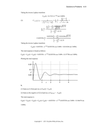
2-6
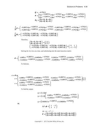
b
theta =
1.0472
/ PI
3 t sin| -- + 4 t | exp(-2 t)
3
/
1/2 2
1/2
1/2
3 3
s
12 s + 6 3
s - 18 3
+ --------- + 24
2
-----------------------------------------2
2
(s + 4 s + 20)
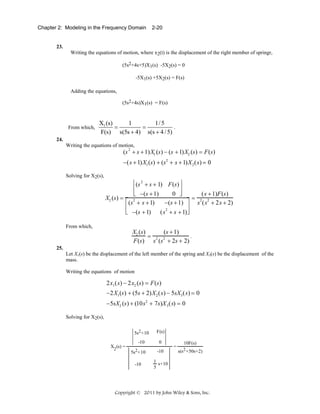
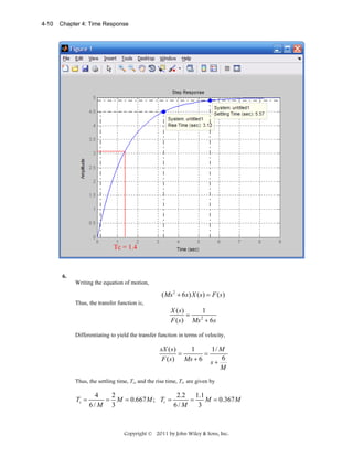
6.
Program:
syms s
'a'
G=(s^2+3*s+10)*(s+5)/[(s+3)*(s+4)*(s^2+2*s+100)];
pretty(G)
g=ilaplace(G);
pretty(g)
'b'
G=(s^3+4*s^2+2*s+6)/[(s+8)*(s^2+8*s+3)*(s^2+5*s+7)];
pretty(G)
g=ilaplace(G);
pretty(g)
Computer response:
ans =
a
2
(s + 5) (s + 3 s + 10)
-------------------------------2
(s + 3) (s + 4) (s + 2 s + 100)
/
1/2
1/2
|
1/2
11
sin(3 11
t) |
5203 exp(-t) | cos(3 11
t) - -------------------- |
20 exp(-3 t)
7 exp(-4 t)
57233
/
------------ - ----------- + -----------------------------------------------------103
54
5562
Copyright © 2011 by John Wiley & Sons, Inc.](https://image.slidesharecdn.com/solutionscontrolsystemsengineeringbynormannice6ed-130502172814-phpapp02-131105052456-phpapp01/85/Solutions-control-system-sengineering-by-normannice-6ed-130502172814-phpapp02-24-320.jpg)
![Chapter 2: Modeling in the Frequency Domain
2-8
Cross multiplying, (s5+3s4+2s3+4s2+5s+2)C(s) = (s4+2s3+5s2+s+1)R(s).
Taking the inverse Laplace transform assuming zero initial conditions,
d 5 c d 4c d 3 c d 2 c dc
d 4r d 3r
d 2 r dr
+3 4 +2 3 +4 2 +5
+ 2c =
+2 3 +5 2 +
+ r.
dt
dc 5
dt
dt
dt
dt
dt 4
dt
dt
Substituting r(t) = t3,
d 5 c d 4c d 3 c d 2 c dc
+3 4 +2 3 +4 2 +5
+ 2c
dc 5
dt
dt
dt
dt
= 18δ(t) + (36 + 90t + 9t2 + 3t3) u(t).
11.
Taking the Laplace transform of the differential equation, s2X(s)-s+1+2sX(s)-2+3x(s)=R(s).
Collecting terms, (s2+2s+3)X(s) = R(s)+s+1.
Solving for X(s), X(s) =
R( s)
s +1
+ 2
.
s + 2s + 3 s + 2s + 3
2
The block diagram is shown below, where R(s) = 1/s.
12.
Program:
'Factored'
Gzpk=zpk([-15 -26 -72],[0 -55 roots([1 5 30])' roots([1 27 52])'],5)
'Polynomial'
Gp=tf(Gzpk)
Computer response:
ans =
Factored
Zero/pole/gain:
5 (s+15) (s+26) (s+72)
-------------------------------------------s (s+55) (s+24.91) (s+2.087) (s^2 + 5s + 30)
ans =
Polynomial
Transfer function:
5 s^3 + 565 s^2 + 16710 s + 140400
-------------------------------------------------------------------s^6 + 87 s^5 + 1977 s^4 + 1.301e004 s^3 + 6.041e004 s^2 + 8.58e004 s
13.
Program:
'Polynomial'
Gtf=tf([1 25 20 15 42],[1 13 9 37 35 50])
Copyright © 2011 by John Wiley & Sons, Inc.](https://image.slidesharecdn.com/solutionscontrolsystemsengineeringbynormannice6ed-130502172814-phpapp02-131105052456-phpapp01/85/Solutions-control-system-sengineering-by-normannice-6ed-130502172814-phpapp02-26-320.jpg)
![Solutions to Problems 2-9
'Factored'
Gzpk=zpk(Gtf)
Computer response:
ans =
Polynomial
Transfer function:
s^4 + 25 s^3 + 20 s^2 + 15 s + 42
----------------------------------------s^5 + 13 s^4 + 9 s^3 + 37 s^2 + 35 s + 50
ans =
Factored
Zero/pole/gain:
(s+24.2) (s+1.35) (s^2 - 0.5462s + 1.286)
-----------------------------------------------------(s+12.5) (s^2 + 1.463s + 1.493) (s^2 - 0.964s + 2.679)
14.
Program:
numg=[-5 -70];
deng=[0 -45 -55 (roots([1 7 110]))' (roots([1 6 95]))'];
[numg,deng]=zp2tf(numg',deng',1e4);
Gtf=tf(numg,deng)
G=zpk(Gtf)
[r,p,k]=residue(numg,deng)
Computer response:
Transfer function:
10000 s^2 + 750000 s + 3.5e006
------------------------------------------------------------------------------s^7 + 113 s^6 + 4022 s^5 + 58200 s^4 + 754275 s^3 + 4.324e006 s^2 + 2.586e007 s
Zero/pole/gain:
10000 (s+70) (s+5)
-----------------------------------------------s (s+55) (s+45) (s^2 + 6s + 95) (s^2 + 7s + 110)
r =
-0.0018
0.0066
0.9513
0.9513
-1.0213
-1.0213
0.1353
p =
+
+
0.0896i
0.0896i
0.1349i
0.1349i
-55.0000
-45.0000
-3.5000
-3.5000
-3.0000
-3.0000
0
k =
+
+
-
9.8869i
9.8869i
9.2736i
9.2736i
[]
Copyright © 2011 by John Wiley & Sons, Inc.](https://image.slidesharecdn.com/solutionscontrolsystemsengineeringbynormannice6ed-130502172814-phpapp02-131105052456-phpapp01/85/Solutions-control-system-sengineering-by-normannice-6ed-130502172814-phpapp02-27-320.jpg)
![Chapter 2: Modeling in the Frequency Domain
2-10
15.
Program:
syms s
'(a)'
Ga=45*[(s^2+37*s+74)*(s^3+28*s^2+32*s+16)]...
/[(s+39)*(s+47)*(s^2+2*s+100)*(s^3+27*s^2+18*s+15)];
'Ga symbolic'
pretty(Ga)
[numga,denga]=numden(Ga);
numga=sym2poly(numga);
denga=sym2poly(denga);
'Ga polynimial'
Ga=tf(numga,denga)
'Ga factored'
Ga=zpk(Ga)
'(b)'
Ga=56*[(s+14)*(s^3+49*s^2+62*s+53)]...
/[(s^2+88*s+33)*(s^2+56*s+77)*(s^3+81*s^2+76*s+65)];
'Ga symbolic'
pretty(Ga)
[numga,denga]=numden(Ga);
numga=sym2poly(numga);
denga=sym2poly(denga);
'Ga polynimial'
Ga=tf(numga,denga)
'Ga factored'
Ga=zpk(Ga)
Computer response:
ans =
(a)
ans =
Ga symbolic
2
3
2
(s + 37 s + 74) (s + 28 s + 32 s + 16)
45 ----------------------------------------------------------2
3
2
(s + 39) (s + 47) (s + 2 s + 100) (s + 27 s + 18 s + 15)
ans =
Ga polynimial
Transfer function:
45 s^5 + 2925 s^4 + 51390 s^3 + 147240 s^2 + 133200 s + 53280
-------------------------------------------------------------------------------s^7 + 115 s^6 + 4499 s^5 + 70700 s^4 + 553692 s^3 + 5.201e006 s^2 + 3.483e006 s
+ 2.75e006
ans =
Ga factored
Zero/pole/gain:
45 (s+34.88) (s+26.83) (s+2.122) (s^2 + 1.17s + 0.5964)
----------------------------------------------------------------(s+47) (s+39) (s+26.34) (s^2 + 0.6618s + 0.5695) (s^2 + 2s + 100)
Copyright © 2011 by John Wiley & Sons, Inc.](https://image.slidesharecdn.com/solutionscontrolsystemsengineeringbynormannice6ed-130502172814-phpapp02-131105052456-phpapp01/85/Solutions-control-system-sengineering-by-normannice-6ed-130502172814-phpapp02-28-320.jpg)
![Solutions to Problems 2-17
⎡ 6s 2 + 12s + 5 ⎤
1
⎡ 1 ⎤
⎢12s 2 + 14 s + 4 ⎥ V1 ( s ) − ⎢ 6 s + 4 ⎥ Vo ( s ) = 2 V ( s )
⎣
⎦
⎣
⎦
2
⎡ 24s + 43s + 54 ⎤
s
⎡ 1 ⎤
−⎢
V1 ( s ) + ⎢
⎥ Vo ( s ) = V ( s )
9
⎣ 6s + 4 ⎥
⎦
⎣ 216s + 144 ⎦
b.
Program:
syms s V
%Construct symbolic object for frequency
%variable 's' and V.
'Mesh Equations'
A2=[(4+4*s) V -2
-(2+4*s) 0 -(4+6*s)
-2 0 (6+6*s+(9/s))]
A=[(4+4*s) -(2+4*s) -2
-(2+4*s) (14+10*s) -(4+6*s)
-2 -(4+6*s) (6+6*s+(9/s))]
I2=det(A2)/det(A);
Gi=I2/V;
G=8*Gi;
G=collect(G);
'G(s) via Mesh Equations'
pretty(G)
%Form Ak = A2.
%Form A.
%Use Cramer's Rule to solve for I2.
%Form transfer function, Gi(s) = I2(s)/V(s).
%Form transfer function, G(s) = 8*I2(s)/V(s).
%Simplify G(s).
%Display label.
%Pretty print G(s)
'Nodal Equations'
A2=[(6*s^2+12*s+5)/(12*s^2+14*s+4) V/2
-1/(6*s+4) s*(V/9)]
%Form Ak = A2.
A=[(6*s^2+12*s+5)/(12*s^2+14*s+4) -1/(6*s+4)
-1/(6*s+4) (24*s^2+43*s+54)/(216*s+144)]
%Form A.
Vo=simple(det(A2))/simple(det(A));
%Use Cramer's Rule to solve for Vo.
G1=Vo/V;
%Form transfer function, G1(s) = Vo(s)/V(s).
G1=collect(G1);
%Simplify G1(s).
'G(s) via Nodal Equations'
%Display label.
pretty(G1)
%Pretty print G1(s)
Computer response:
Copyright © 2011 by John Wiley & Sons, Inc.](https://image.slidesharecdn.com/solutionscontrolsystemsengineeringbynormannice6ed-130502172814-phpapp02-131105052456-phpapp01/85/Solutions-control-system-sengineering-by-normannice-6ed-130502172814-phpapp02-35-320.jpg)
![Chapter 2: Modeling in the Frequency Domain
2-18
ans =
Mesh Equations
A2 =
[
4*s + 4, V,
-2]
[ - 4*s - 2, 0,
- 6*s - 4]
[
-2, 0, 6*s + 9/s + 6]
A =
[
4*s + 4, - 4*s - 2,
-2]
[ - 4*s - 2, 10*s + 14,
- 6*s - 4]
[
-2, - 6*s - 4, 6*s + 9/s + 6]
ans =
G(s) via Mesh Equations
3
2
48 s + 96 s + 112 s + 36
---------------------------3
2
48 s + 150 s + 220 s + 117
ans =
Nodal Equations
A2 =
[ (6*s^2 + 12*s + 5)/(12*s^2 + 14*s + 4),
V/2]
[
-1/(6*s + 4), (V*s)/9]
A =
[ (6*s^2 + 12*s + 5)/(12*s^2 + 14*s + 4),
-1/(6*s + 4)]
[
-1/(6*s + 4), (24*s^2 + 43*s + 54)/(216*s + 144)]
ans =
G(s) via Nodal Equations
3
2
48 s + 96 s + 112 s + 36
---------------------------3
2
48 s + 150 s + 220 s + 117
Copyright © 2011 by John Wiley & Sons, Inc.](https://image.slidesharecdn.com/solutionscontrolsystemsengineeringbynormannice6ed-130502172814-phpapp02-131105052456-phpapp01/85/Solutions-control-system-sengineering-by-normannice-6ed-130502172814-phpapp02-36-320.jpg)
![Chapter 2: Modeling in the Frequency Domain
2-24
(Jeqs2+Deqs)θ3(s) = T(s) (
N4 N2
)
N3 N1
Thus,
N 4N 2
θ 3 (s)
N3 N1
=
2
T (s) Jeq s + Deqs
where
⎛N ⎞2
⎛N N ⎞2
4⎟
4 2⎟
⎟ + J1 ⎜
⎜
⎟ , and
⎝ N3 ⎠
⎝ N3 N1 ⎠
Jeq = J4+J5+(J2+J3) ⎜
⎜
Deq = (D4 + D5 ) + (D2 + D3 )(
33.
N4 2
NN
) + D1 ( 4 2 ) 2
N3
N 3 N1
Reflecting all impedances to θ2(s),
2
2
2
2
2
N
{[J2+J1(N2 ) +J3 (N3 ) ]s2 + [f2+f1(N2 ) +f3(N43 ) ]s + [K(N3 ) ]}θ2(s) = T(s)N2
N1
N1
N4
N1
N4
Substituting values,
2
2
2
{[1+2(3)2+16(1 ) ]s2 + [2+1(3)2+32(1 ) ]s + 64(1 ) }θ2(s) = T(s)(3)
4
4
4
Thus,
θ2(s)
3
T(s) = 20s2+13s+4
34.
Reflecting impedances to θ2,
⎡
⎡
⎛ ⎞2
⎛
⎞2⎤
⎛
⎞2⎤ ⎡
⎛ ⎞2⎤ ⎛ ⎞
⎢200 + 3⎜ 50 ⎟ + 200⎜ 5 x 50 ⎟ ⎥ s 2 + ⎢1000⎜ 5 x 50 ⎟ ⎥ s + ⎢250 + 3⎜ 50 ⎟ ⎥ = ⎜ 50 ⎟ T (s)
⎝ 5⎠
⎝ 25 5 ⎠ ⎦
⎝ 25 5 ⎠ ⎦ ⎣
⎝ 5 ⎠ ⎦ ⎝ 5⎠
⎢
⎥
⎢
⎥ ⎢
⎥
⎣
⎣
Thus,
θ 2 (s)
T( s)
=
10
1300s + 4000s + 550
2
35.
Reflecting impedances and applied torque to respective sides of the spring yields the following
equivalent circuit:
Copyright © 2011 by John Wiley & Sons, Inc.](https://image.slidesharecdn.com/solutionscontrolsystemsengineeringbynormannice6ed-130502172814-phpapp02-131105052456-phpapp01/85/Solutions-control-system-sengineering-by-normannice-6ed-130502172814-phpapp02-42-320.jpg)
![Chapter 2: Modeling in the Frequency Domain
2-26
−2s
3T ( s )
s ( s + 2)
−2s
(2s + 3)
0
0
−3
0
18T ( s )
θ 4 ( s) =
=
−2 s
0
s ( s + 2)
s (2s 2 + 9s + 6)
−2s
−3
(2s + 3)
−3
0
( s + 3)
But, θ L (s) = 5θ 4 (s) . Hence,
θ 4 ( s)
T ( s)
=
90
s (2s + 9 s + 6)
2
37.
Reflect all impedances on the right to the viscous damper and reflect all impedances and torques on the
left to the spring and obtain the following equivalent circuit:
Writing the equations of motion,
(J1eqs2+K)θ2(s) -Kθ3(s) = Teq(s)
-Kθ2(s)+(Ds+K)θ3(s) -Dsθ4(s) = 0
-Dsθ3(s) +[J2eqs2 +(D+Deq)s]θ4(s) = 0
N2
where: J1eq = J2+(Ja+J1) N
1
( )
2
N3
; J2eq = J3+(JL+J4) N
4
( )
2
N3
; Deq = DL N
4
N1
N2 .
Copyright © 2011 by John Wiley & Sons, Inc.
( )
2
; θ2(s) = θ1(s)](https://image.slidesharecdn.com/solutionscontrolsystemsengineeringbynormannice6ed-130502172814-phpapp02-131105052456-phpapp01/85/Solutions-control-system-sengineering-by-normannice-6ed-130502172814-phpapp02-44-320.jpg)
![Solutions to Problems 2-27
38.
Reflect impedances to the left of J5 to J5 and obtain the following equivalent circuit:
Writing the equations of motion,
[Jeqs2+(Deq+D)s+(K2+Keq)]θ5(s)
-[Ds+K2]θ6(s) = 0
-[K2+Ds]θ5(s) + [J6s2+2Ds+K2]θ6(s) = T(s)
From the first equation,
θ6(s) Jeqs2+(Deq+D)s+ (K2+Keq)
θ5(s) N1N3
=
. But,
=
. Therefore,
Ds+K2
θ5(s)
θ1(s) N2N4
θ6(s) N1N3 ⎛ Jeqs2+(Deq+D)s+ (K2+Keq) ⎞
=
⎜
⎟ ,
Ds+K2
⎠
θ1(s) N2N4 ⎝
N4N2
where Jeq = J1 N N
3 1
[ (
Deq = D
[(N4N2 )
N3N1
2
)
2
N4
+ (J2+J3) N
3
N4
+ N
3
( )
( )
2
2
N4
+ (J4+J5) , Keq = K1 N
3
]
]
+1 .
39.
Draw the freebody diagrams,
Copyright © 2011 by John Wiley & Sons, Inc.
( )
2
, and](https://image.slidesharecdn.com/solutionscontrolsystemsengineeringbynormannice6ed-130502172814-phpapp02-131105052456-phpapp01/85/Solutions-control-system-sengineering-by-normannice-6ed-130502172814-phpapp02-45-320.jpg)
![Chapter 2: Modeling in the Frequency Domain
2-28
Write the equations of motion from the translational and rotational freebody diagrams,
-fvrsθ(s) = F(s)
(Ms2+2fv s+K2)X(s)
-fvrsX(s) +(Js2+fvr2s)θ(s) = 0
Solve for θ(s),
Ms 2+2fvs+K
θ(s) =
2
F(s)
-fvrs
Ms 2+2fvs+K
-fvrs
θ(s)
From which, F(s) =
0
=
2
-fvrs
fvrF(s)
2
3
JMs +(2Jfv+Mfvr2)s 2+(JK +fvr2)s+K fvr2
2
2
2
Js +fvr2s
fvr
JMs3+(2Jfv+Mfvr2)s2+(JK2+fv2r2)s+K2fvr2
.
40.
Draw a freebody diagram of the translational system and the rotating member connected to the
translational system.
2
3
2
From the freebody diagram of the mass, F(s) = (2s2+2s+3)X(s). Summing torques on the rotating
member,
(Jeqs2 +Deqs)θ(s) + F(s)2 = Teq(s). Substituting F(s) above, (Jeqs2 +Deqs)θ(s) + (4s2+4s+6)X(s) =
X(s)
Teq(s). However, θ(s) = 2 . Substituting and simplifying,
Jeq
Deq
+4 s2 + 2 +4 s+6 X(s)
Teq =
2
[(
) (
) ]
But, Jeq = 3+3(4)2 = 51, Deq = 1(2)2 +1 = 5, and Teq(s) = 4T(s). Therefore,
Copyright © 2011 by John Wiley & Sons, Inc.](https://image.slidesharecdn.com/solutionscontrolsystemsengineeringbynormannice6ed-130502172814-phpapp02-131105052456-phpapp01/85/Solutions-control-system-sengineering-by-normannice-6ed-130502172814-phpapp02-46-320.jpg)
![Solutions to Problems 2-29
[ 59 s2 + 13 s+6]X(s) = 4T(s). Finally, X(s)
T(s)
2
2
=
8
.
59 s + 13s + 12
2
41.
Writing the equations of motion,
(J1s2+K1)θ1(s)
- K1θ2(s)
= T(s)
2+D s+K )θ (s) +F(s)r -D sθ (s) = 0
-K1θ1(s) + (J2s
3
1 2
3 3
2+D s)θ (s) = 0
-D3sθ2(s) + (J2s
3 3
where F(s) is the opposing force on J2 due to the translational member and r is the radius of J2. But,
for the translational member,
F(s) = (Ms2+fvs+K2)X(s) = (Ms2+fvs+K2)rθ(s)
Substituting F(s) back into the second equation of motion,
(J1s2+K1)θ1(s)
- K1θ2(s)
= T(s)
-K1θ1(s) + [(J2 + Mr2)s2+(D3 + fvr2)s+(K1 + K2r2)]θ2(s)
-D3sθ3(s) = 0
-D3sθ2(s) + (J2s2+D3s)θ3(s) = 0
Notice that the translational components were reflected as equivalent rotational components by the
square of the radius. Solving for θ2(s), θ 2 (s ) =
K1 ( J3 s 2 + D3 s)T( s)
, where Δ is the
Δ
determinant formed from the coefficients of the three equations of motion. Hence,
θ 2 (s)
K1 (J3 s2 + D3 s)
=
T(s)
Δ
Since
X(s) = rθ 2 (s),
X(s) rK1 (J 3 s2 + D3 s)
=
T (s)
Δ
42.
Kt Tstall 100
Ea
50 1
=
=
= 2 ; Kb =
=
=
Ra Ea
ω no− load 150 3
50
Also,
Jm = 5+18
Thus,
θ m (s )
Ea (s)
Since θL(s) =
=
(1)
3
2
2
= 7; Dm = 8+36
( 1 ) = 12.
3
2/7
2/7
=
1
2
38
s ( s + (12 + )) s ( s + )
7
3
21
1
θm(s),
3
Copyright © 2011 by John Wiley & Sons, Inc.](https://image.slidesharecdn.com/solutionscontrolsystemsengineeringbynormannice6ed-130502172814-phpapp02-131105052456-phpapp01/85/Solutions-control-system-sengineering-by-normannice-6ed-130502172814-phpapp02-47-320.jpg)
![Chapter 2: Modeling in the Frequency Domain
2-32
47.
The equations of motion in terms of velocity are:
K1 K2
K
+ ]V1 (s) − 2 V2 (s) − fv 3V3 (s) = 0
s
s
s
K
K
− 2 V1 (s) + [M2 s + ( fv 2 + f v 4 ) + 2 ]V2 (s) − f v4 V3 (s) = F(s)
s
s
− f v3 V1 (s) − f v4 V2 (s) + [M3 s + fV 3 + fv 4 ]V3 (S) = 0
[M1s + ( fv1 + fv 3 ) +
For the series analogy, treating the equations of motion as mesh equations yields
In the circuit, resistors are in ohms, capacitors are in farads, and inductors are in henries.
For the parallel analogy, treating the equations of motion as nodal equations yields
In the circuit, resistors are in ohms, capacitors are in farads, and inductors are in henries.
48.
Writing the equations of motion in terms of angular velocity, Ω(s) yields
Copyright © 2011 by John Wiley & Sons, Inc.](https://image.slidesharecdn.com/solutionscontrolsystemsengineeringbynormannice6ed-130502172814-phpapp02-131105052456-phpapp01/85/Solutions-control-system-sengineering-by-normannice-6ed-130502172814-phpapp02-50-320.jpg)
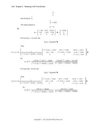
![3-2 Chapter 3: Modeling in the Time Domain
Aquifer: State-Space Representation
dh1
C1 dt = qi1-qo1+q2-q1+q21 = qi1-0+G2(h2-h1)-G1h1+G21(H1-h1) =
-(G2+G1+G21)h1+G2h2+qi1+G21H1
dh2
C2 dt = qi2-q02+q3-q2+q32 = qi2-qo2+G3(h3-h2)-G2(h2-h1)+0 = G2h1-[G2+G3]h2+G3h3+qi2-qo2
dh3
C3 dt = qi3-qo3+q4-q3+q43 = qi3-qo3+0-G3(h3-h2)+0 = G3h2-G3h3+qi3-qo3
Dividing each equation by Ci and defining the state vector as x = [h1 h2 h3]T
⎡ −(G1 + G2 + G3 )
⎢
C1
.
G2
⎢
x=
C2
⎢
⎢
0
⎣
⎡1 0
y = ⎢0 1
⎢0 0
⎣
G2
C1
−(G2 + G3 )
C2
G3
C3
⎤
⎡ qi1 + G21 H1 ⎤
⎥
⎢
⎥
C1
G3 ⎥
⎢ qi 2 − qo2 ⎥
x+
u(t)
C2 ⎥
C2
⎢
⎥
−G3 ⎥
⎢ qi3 − qo3 ⎥
C3 ⎦
C3
⎣
⎦
0
0⎤
0⎥ x
1⎥
⎦
where u(t) = unit step function.
ANSWERS TO REVIEW QUESTIONS
1. (1) Can model systems other than linear, constant coefficients; (2) Used for digital simulation
2. Yields qualitative insight
3. That smallest set of variables that completely describe the system
4. The value of the state variables
5. The vector whose components are the state variables
6. The n-dimensional space whose bases are the state variables
7. State equations, an output equation, and an initial state vector (initial conditions)
8. Eight
9. Forms linear combinations of the state variables and the input to form the desired output
10. No variable in the set can be written as a linear sum of the other variables in the set.
11. (1) They must be linearly independent; (2) The number of state variables must agree with the order of
the differential equation describing the system; (3) The degree of difficulty in obtaining the state equations
for a given set of state variables.
12. The variables that are being differentiated in each of the linearly independent energy storage elements
Copyright © 2011 by John Wiley & Sons, Inc.](https://image.slidesharecdn.com/solutionscontrolsystemsengineeringbynormannice6ed-130502172814-phpapp02-131105052456-phpapp01/85/Solutions-control-system-sengineering-by-normannice-6ed-130502172814-phpapp02-69-320.jpg)
![3-4 Chapter 3: Modeling in the Time Domain
Solving for i1
i1 =
2
1
1
1
i2 + i4 − vo + vi
3
3
3
3
Thus,
2
1
1
2
v1 = vi − i1 = − i2 − i4 + vo + vi
3
3
3
3
Also,
1
1
1
1
i3 = i1 − i2 = − i2 + i4 − vo + vi
3
3
3
3
and
1
2
1
1
i 5 = i3 − i4 = − i2 − i4 − vo + vi
3
3
3
3
Finally,
1
2
2
1
v 2 = i5 + vo = − i2 − i 4 + vo + vi
3
3
3
3
Using v1, v2, and i5, the state equation is
⎡ 2
⎢−
⎢ 3
•
1
x = ⎢−
⎢ 3
⎢ 1
⎢−
⎣ 3
y = [0
⎡2 ⎤
1 ⎤
⎥
⎢ ⎥
3 ⎥
⎢ 3⎥
2 ⎥
⎢1 ⎥
⎥ x + ⎢ 3 ⎥ vi
3 ⎥
⎢1 ⎥
1
⎢ ⎥
− ⎥
⎣ 3⎦
3⎦
1
3
2
−
3
2
−
3
−
0 1]x
2.
Add branch currents and node voltages to the schematic and obtain,
3
3
2
3
Write the differential equation for each energy storage element.
Copyright © 2011 by John Wiley & Sons, Inc.](https://image.slidesharecdn.com/solutionscontrolsystemsengineeringbynormannice6ed-130502172814-phpapp02-131105052456-phpapp01/85/Solutions-control-system-sengineering-by-normannice-6ed-130502172814-phpapp02-71-320.jpg)
![3-5 Chapter 3: Modeling in the Time Domain
dv1 1
= i2
dt 3
di3 1
= vL
dt 2
Therefore the state vector is
⎡v1 ⎤
x=⎢ ⎥
⎢ i3 ⎦
⎣ ⎥
Now obtain v L and i2 , in terms of the state variables,
vL = v1 − v2 = v1 − 3iR = v1 − 3(i3 + 4v1 ) = −11v1 − 3i3
1
1
1
i2 = i1 − i3 = (vi − v1 ) − i3 = − v1 − i3 + vi
3
3
3
Also, the output is
y = iR = 4v1 + i3
Hence,
1⎤
⎡ 1
⎡1⎤
⎢ − 9 − 3⎥
x=⎢
⎥ x + ⎢ 9 ⎥ vi
⎢ ⎥
⎢ − 11 − 3 ⎥
⎢0⎥
⎣ ⎦
⎢ 2
2⎥
⎣
⎦
y = [ 4 1] x
•
3.
Let C1 be the grounded capacitor and C 2 be the other. Now, writing the equations for the energy
storage components yields,
di L
= v i − vC 1
dt
dv C1
= i1 − i2
(1)
dt
dv C2
= i2 − i3
dt
⎡i ⎤
⎢ L⎥
Thus the state vector is x = ⎢ vC1 ⎥ . Now, find the three loop currents in terms of the state variables
⎢ ⎥
⎢vC2 ⎦
⎣ ⎥
and the input.
Writing KVL around Loop 2 yields vC 1 = vC 2 + i2 .Or,
i2 = vC 1 − vC 2
Copyright © 2011 by John Wiley & Sons, Inc.](https://image.slidesharecdn.com/solutionscontrolsystemsengineeringbynormannice6ed-130502172814-phpapp02-131105052456-phpapp01/85/Solutions-control-system-sengineering-by-normannice-6ed-130502172814-phpapp02-72-320.jpg)
![3-6 Chapter 3: Modeling in the Time Domain
Writing KVL around the outer loop yields i3 + i2 = vi Or,
i3 = vi − i2 = vi − vC1 + vC2
Also, i1 − i3 = iL . Hence,
i1 = iL + i3 = i L + vi − v C1 + vC 2
Substituting the loop currents in equations (1) yields the results in vector-matrix form,
⎡ di ⎤
⎢ L ⎥
⎢ dt ⎥ ⎡ 0 −1 0 ⎤ ⎡ i L ⎤ ⎡ 1 ⎤
⎥⎢ ⎥ ⎢ ⎥
⎢ dvC1 ⎥ ⎢
= ⎢ 1 − 2 2 ⎥ ⎢ vC1 ⎥ + ⎢ 1 ⎥ vi
⎢
⎥
⎢ dt ⎥ ⎢ 0 2 − 2⎥ ⎢v ⎥ ⎢ − 1⎥
⎦ ⎢ C2 ⎥ ⎣ ⎦
⎣ ⎦
⎢ dv C2 ⎥ ⎣
⎢ dt ⎥
⎣
⎦
Since vo = i2 = vC1 − vC 2 , the output equation is
⎡ ⎤
⎢ iL ⎥
y = [0 1 1]⎢ v C1 ⎥
⎢ ⎥
⎢ vC 2 ⎦
⎣ ⎥
4.
Equations of motion in Laplace:
(2 s 2 + 3s + 2) X 1 ( s ) − ( s + 2) X 2 ( s ) − sX 3 ( s ) = 0
−( s + 2) X 1 ( s ) + ( s 2 + 2 s + 2) X 2 ( s) − sX 3 ( s) = F ( s)
− sX 1 ( s ) − sX 2 ( s ) + ( s 2 + 3s ) X 3 ( s ) = 0
Equations of motion in the time domain:
dx
d 2 x1
dx
dx
2 2 + 3 1 + 2 x1 − 2 − 2 x2 − 3 = 0
dt
dt
dt
dt
2
dx
d x
dx
dx
− 1 − 2 x1 + 22 + 2 2 + 2 x2 − 3 = f (t )
dt
dt
dt
dt
2
dx
dx dx d x
− 1 − 2 + 23 + 3 3 = 0
dt
dt
dt
dt
Define state variables:
Copyright © 2011 by John Wiley & Sons, Inc.](https://image.slidesharecdn.com/solutionscontrolsystemsengineeringbynormannice6ed-130502172814-phpapp02-131105052456-phpapp01/85/Solutions-control-system-sengineering-by-normannice-6ed-130502172814-phpapp02-73-320.jpg)

![3-8 Chapter 3: Modeling in the Time Domain
1
0
0 0 0 ⎤
⎡0
⎡0⎤
⎢ −1 −1.5 1 0.5 0 0.5⎥
⎢0⎥
⎢
⎥
⎢ ⎥
•
⎢0
⎢0 ⎥
0
0
1 0 0 ⎥
Z=⎢
⎥ Z + ⎢ ⎥ f (t )
−2 − 2 0 1 ⎥
1
⎢2
⎢1 ⎥
⎢0
⎢0 ⎥
0
0
0 0 1 ⎥
⎢
⎥
⎢ ⎥
1
0
1 0 −3 ⎥
⎢
⎢ ⎦
⎣0
⎦
⎣0 ⎥
y = [ 0 0 0 0 1 0] Z
5.
Writing the equations of motion,
(2s 2 + 2s + 1) X 1 ( s) − sX 2 ( s ) − ( s + 1) X 3 ( s ) = 0
− sX 1 ( s ) + ( s 2 + 2s + 1) X 2 ( s) − ( s + 1) X 3 ( s) = 0
−( s + 1) X 1 ( s ) − ( s + 1) X 2 ( s ) + ( s 2 + 2s + 2) X 3 ( s ) = F ( s )
Taking the inverse Laplace transform,
••
•
•
•
2 x1 + 2 x1 + x1 − x2 − x3 − x3 = 0
•
••
•
•
− x1 + x2 + 2 x2 + x2 − x3 − x3 = 0
•
•
••
•
− x1 − x1 − x2 − x2 + x3 + 2 x3 + 2 x3 = f (t )
Simplifying,
••
•
x1 = − x1 −
••
•
••
•
1
1 • 1 • 1
x1 + x2 + x3 + x3
2
2
2
2
•
•
x2 = x1 − 2 x2 − x2 + x3 + x3
•
•
x3 = x1 + x1 + x2 + x2 − 2 x3 − 2 x3 + f (t )
Defining the state variables,
•
•
•
z1 = x1 ; z2 = x1 ; z3 = x2 ; z4 = x2 ; z 5 = x 3 ; z 6 = x3
Writing the state equations using the simplified equations above yields,
Copyright © 2011 by John Wiley & Sons, Inc.](https://image.slidesharecdn.com/solutionscontrolsystemsengineeringbynormannice6ed-130502172814-phpapp02-131105052456-phpapp01/85/Solutions-control-system-sengineering-by-normannice-6ed-130502172814-phpapp02-75-320.jpg)
![3-9 Chapter 3: Modeling in the Time Domain
•
•
z1 = x1 = z2
•
••
1
1
1
1
z2 = x1 = − z2 − z1 + z4 + z6 + z5
2
2
2
2
•
•
•
••
•
•
z3 = x2 = z4
z4 = x2 = z2 − 2 z4 − z3 + z6 + z5
z5 = x3 = z6
•
••
z6 = x3 = z2 + z1 + z4 + z3 − 2 z6 − 2 z5 + f (t )
Converting to vector-matrix form,
⎡ 0
⎢ 1
⎢−
⎢ 2
•
z=⎢ 0
⎢
⎢ 0
⎢ 0
⎢
⎢ 1
⎣
0 0 0⎤
⎡0⎤
1 1 1⎥
⎢0⎥
⎥
−1 0
⎢ ⎥
2 2 2⎥
⎢0⎥
0 0 1 0 0 ⎥ z + ⎢ ⎥ f (t )
⎥
⎢0⎥
1 −1 − 2 1 1 ⎥
⎢0⎥
0 0 0 0 1⎥
⎢ ⎥
⎥
⎢1 ⎥
⎣ ⎦
1 1 1 −2 − 2 ⎥
⎦
1
0
y = [1 0 0 0 0 0] z
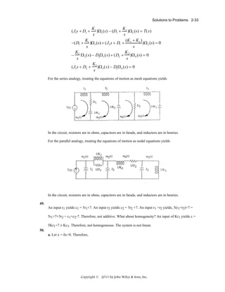
6.
Drawing the equivalent network,
3.33 T
555.56
Writing the equations of motion,
(555.56s 2 + 100)θ 2 − 100θ3 = 3.33T
−100θ 2 + (100s 2 + 100s + 100)θ3 = 0
Taking the inverse Laplace transform and simplifying,
Copyright © 2011 by John Wiley & Sons, Inc.](https://image.slidesharecdn.com/solutionscontrolsystemsengineeringbynormannice6ed-130502172814-phpapp02-131105052456-phpapp01/85/Solutions-control-system-sengineering-by-normannice-6ed-130502172814-phpapp02-76-320.jpg)
![3-10 Chapter 3: Modeling in the Time Domain
••
θ 2 + 0.18θ 2 − 0.18θ 3 = 0.006T
••
•
−θ 2 + θ3 + θ3 + θ 3 = 0
Defining the state variables as
•
•
x1 = θ2 , x 2 = θ 2 , x3 = θ3 , x 4 = θ 3
Writing the state equations using the equations of motion and the definitions of the state variables
•
x1 = x2
•
••
x2 = θ 2 = −0.18θ 2 + 0.18θ 3 + 0.006T = −0.18 x1 + 0.18 x3 + 0.006T
•
x3 = x4
•
,
••
•
x4 = θ3 = θ 2 − θ3 − θ3 = x1 − x3 − x4
y = 3.33θ 2 = 3.33x1
In vector-matrix form,
⎡ 0
⎢ −0.18
•
x=⎢
⎢ 0
⎢
⎣ 1
1
0
0⎤
⎡ 0 ⎤
⎥
⎢0.006 ⎥
0 0.18 0 ⎥
⎥T
x+⎢
⎢ 0 ⎥
0
0
1⎥
⎥
⎢
⎥
0 −1 −1⎦
⎣ 0 ⎦
y = [3.33 0 0 0] x
7.
Drawing the equivalent circuit,
10T
(1/10)(102 ) = 10 N-m/rad
Writing the equations of motion,
Copyright © 2011 by John Wiley & Sons, Inc.
200(1/10)2 =2 N-m/rad](https://image.slidesharecdn.com/solutionscontrolsystemsengineeringbynormannice6ed-130502172814-phpapp02-131105052456-phpapp01/85/Solutions-control-system-sengineering-by-normannice-6ed-130502172814-phpapp02-77-320.jpg)
![3-12 Chapter 3: Modeling in the Time Domain
9.
a. . Using the standard form derived in the textbook,
1
0
0 ⎤
⎡ 0
⎡ 0⎤
•
⎢ 0
⎢ 0⎥
0
1
0 ⎥
r( t )
x=
x+
⎢ 0
⎢ 0⎥
0
0
1 ⎥
⎢− 100 −7 − 10 −20 ⎥
⎢ 1⎥
⎣
⎦
⎣ ⎦
c = [100 0 0 0]x
b. Using the standard form derived in the textbook,
1 0 0 0⎤
⎡ 0
⎡0 ⎤
⎢ 0
⎢0 ⎥
0 1 0 0⎥
•
x=⎢ 0
0 0 1 0 ⎥ x + ⎢0 ⎥ r(t )
⎢ 0
⎢0 ⎥
0 0 0 1⎥
⎢
⎥
⎢ ⎥
⎣− 30 −1 −6 −9 −8⎦
⎣1 ⎦
c = [30 0 0 0 0]x
10.
Program:
'a'
num=100;
den=[1 20 10 7 100];
G=tf(num,den)
[Acc,Bcc,Ccc,Dcc]=tf2ss(num,den);
Af=flipud(Acc);
A=fliplr(Af)
B=flipud(Bcc)
C=fliplr(Ccc)
'b'
num=30;
den=[1 8 9 6 1 30];
G=tf(num,den)
[Acc,Bcc,Ccc,Dcc]=tf2ss(num,den);
Af=flipud(Acc);
A=fliplr(Af)
B=flipud(Bcc)
C=fliplr(Ccc)
Computer response:
ans =
a
Transfer function:
100
--------------------------------s^4 + 20 s^3 + 10 s^2 + 7 s + 100
A =
0
0
0
-100
1
0
0
-7
0
1
0
-10
0
0
1
-20
Copyright © 2011 by John Wiley & Sons, Inc.](https://image.slidesharecdn.com/solutionscontrolsystemsengineeringbynormannice6ed-130502172814-phpapp02-131105052456-phpapp01/85/Solutions-control-system-sengineering-by-normannice-6ed-130502172814-phpapp02-79-320.jpg)
![3-13 Chapter 3: Modeling in the Time Domain
B =
0
0
0
1
C =
100
0
0
0
ans =
b
Transfer function:
30
-----------------------------------s^5 + 8 s^4 + 9 s^3 + 6 s^2 + s + 30
A =
0
0
0
0
-30
1
0
0
0
-1
0
1
0
0
-6
0
0
1
0
-9
0
0
0
1
-8
0
0
0
0
B =
0
0
0
0
1
C =
30
11.
a. Using the standard form derived in the textbook,
⎡ 0
⎢ 0
x=⎢
⎢ 0
⎢
⎣ −13
c = [10 8
•
0⎤
⎡0⎤
⎥
⎢0⎥
0⎥
x + ⎢ ⎥ r (t )
⎢0⎥
0 0 1⎥
⎥
⎢ ⎥
−5 − 1 −5 ⎦
⎣1 ⎦
0 0 0] x
1
0
0
1
Copyright © 2011 by John Wiley & Sons, Inc.](https://image.slidesharecdn.com/solutionscontrolsystemsengineeringbynormannice6ed-130502172814-phpapp02-131105052456-phpapp01/85/Solutions-control-system-sengineering-by-normannice-6ed-130502172814-phpapp02-80-320.jpg)
![3-14 Chapter 3: Modeling in the Time Domain
b. Using the standard form derived in the textbook,
⎡0
⎢0
⎢
•
x = ⎢0
⎢
⎢0
⎢0
⎣
1
0
0
0
0
0⎤
⎡0⎤
⎥
⎢0⎥
1
0
0⎥
⎢ ⎥
0
1
0 ⎥ x + ⎢0⎥ r (t )
⎥
⎢ ⎥
0
0
1⎥
⎢0⎥
⎢1 ⎥
−8 −13 −9 ⎥
⎦
⎣ ⎦
0
0
c = [ 6 7 12 2 1] x
12.
Program:
'a'
num=[8 10];
den=[1 5 1 5 13]
G=tf(num,den)
[Acc,Bcc,Ccc,Dcc]=tf2ss(num,den);
Af=flipud(Acc);
A=fliplr(Af)
B=flipud(Bcc)
C=fliplr(Ccc)
'b'
num=[1 2 12 7 6];
den=[1 9 13 8 0 0]
G=tf(num,den)
[Acc,Bcc,Ccc,Dcc]=tf2ss(num,den);
Af=flipud(Acc);
A=fliplr(Af)
B=flipud(Bcc)
C=fliplr(Ccc)
Computer response:
ans =
ans =
a
den =
1
5
1
5
13
Transfer function:
8 s + 10
---------------------------s^4 + 5 s^3 + s^2 + 5 s + 13
A =
0
0
0
-13
1
0
0
-5
0
1
0
-1
0
0
1
-5
Copyright © 2011 by John Wiley & Sons, Inc.](https://image.slidesharecdn.com/solutionscontrolsystemsengineeringbynormannice6ed-130502172814-phpapp02-131105052456-phpapp01/85/Solutions-control-system-sengineering-by-normannice-6ed-130502172814-phpapp02-81-320.jpg)
![3-16 Chapter 3: Modeling in the Time Domain
Writing the differential equation for the first box:
•••
••
•
x + 6 x + 10 x + 5 x = r (t )
Defining the state variables:
x1 = x
•
x2 = x
••
x3 = x
Thus,
•
x1 = x2
•
x2 = x3
•
•
••
x3 = −5 x − 10 x − 6 x + r (t ) = −5 x1 − 10 x2 − 6 x3 + r (t )
From the second box,
••
•
y = x + 3 x + 8 x = 8 x1 + 3 x2 + x3
In vector-matrix form:
1
0⎤
⎡0
⎡0⎤
⎢0
⎥ x + ⎢0 ⎥ r (t )
0
1⎥
x=⎢
⎢ ⎥
⎢ −5 −10 −6 ⎥
⎢1 ⎥
⎣
⎦
⎣ ⎦
y = [8 3 1] x
•
14.
a. G(s)=C(sI-A)-1B
0
0
0
0
1
-3
A=
1
0
-2
-5
;B=
;C= 1
0
0
0
10
s2+5s+2
(sI - A) =
1
2
s3 + 5s + 2s +3
s+5
1
-3
s(s+5)
s
-3s
-1
-2s-3
s2
10
Therefore, G(s) = 3 2
.
s +5s +2s+3
b. G(s)=C(sI-A)-1B
A=
2 3 −8
0 5 3
−3 −5 −4
1
; B = 4 ; C = 1, 3, 6
6
Copyright © 2011 by John Wiley & Sons, Inc.](https://image.slidesharecdn.com/solutionscontrolsystemsengineeringbynormannice6ed-130502172814-phpapp02-131105052456-phpapp01/85/Solutions-control-system-sengineering-by-normannice-6ed-130502172814-phpapp02-83-320.jpg)
![3-17 Chapter 3: Modeling in the Time Domain
s I− A −1 =
s2 − s − 5
1
3 − 3 s 2 − 27 s + 157
s
3 s + 52
−9
s2 + 2 s − 32
3 s− 6
− 5 s+1
s2 − 7 s + 10
− 3 s + 15
− 8 s + 49
2
Therefore, G s = 49 s − 349 s + 452 .
3
2
s − 3 s − 27 s + 157
c. G(s)=C(sI-A)-1B
⎡5⎤
⎡ 3 −5 2 ⎤
A = ⎢ 1 −8 7 ⎥; B = ⎢ −3⎥ ; C = [1 −4 3]
⎢2⎥
⎢ −3 −6 2 ⎥
⎣ ⎦
⎣
⎦
(sI − A) −1
⎡ (s2 + 6s + 26)
−(5s + 2)
(2s − 19) ⎤
1
⎢ (s − 23)
= 3
(7s − 19) ⎥
(s2 − 5s + 12)
s + 3s2 + 19s − 133 ⎢
⎥
−(6s − 33) (s2 + 5s − 19) ⎦
⎣ −(3s + 30)
Therefore, G(s) =
23s2 − 48s − 7
.
s 3 + 3s2 + 19s − 133
15.
Program:
'a'
A=[0 1 5 0;0 0 1 0;0 0 0 1;-7 -9 -2 -3];
B=[0;5;8;2];
C=[1 3 6 6];
D=0;
statespace=ss(A,B,C,D)
[num,den]=ss2tf(A,B,C,D);
G=tf(num,den)
'b'
A=[3 1 0 4 -2;-3 5 -5 2 -1;0 1 -1 2 8;-7 6 -3 -4 0;-6 0 4 -3 1];
B=[2;7;8;5;4];
C=[1 -2 -9 7 6];
D=0;
statespace=ss(A,B,C,D)
[num,den]=ss2tf(A,B,C,D);
G=tf(num,den)
Computer response:
ans =
a
a =
x1
x2
x3
x4
x1
0
0
0
-7
x2
1
0
0
-9
x3
5
1
0
-2
x4
0
0
1
-3
Copyright © 2011 by John Wiley & Sons, Inc.](https://image.slidesharecdn.com/solutionscontrolsystemsengineeringbynormannice6ed-130502172814-phpapp02-131105052456-phpapp01/85/Solutions-control-system-sengineering-by-normannice-6ed-130502172814-phpapp02-84-320.jpg)
![3-19 Chapter 3: Modeling in the Time Domain
0 0 0 1
-7 -9 -2 -3];
B=[0;5;8;2];
C=[1 3 4 6];
D=0;
I=[1 0 0 0
0 1 0 0
0 0 1 0
0 0 0 1];
'T(s)'
T=C*((s*I-A)^-1)*B+D;
T=simple(T);
pretty(T)
'b'
A=[3 1 0 4 -2
-3 5 -5 2 -1
0 1 -1 2 8
-7 6 -3 -4 0
-6 0 4 -3 1];
B=[2;7;6;5;4];
C=[1 -2 -9 7 6];
D=0;
I=[1 0 0 0 0
0 1 0 0 0
0 0 1 0 0
0 0 0 1 0
0 0 0 0 1];
'T(s)'
T=C*((s*I-A)^-1)*B+D;
T=simple(T);
pretty(T)
Computer response:
ans =
a
ans =
T(s)
2
3
-164 s - 1621 s - 260 + 59 s
-----------------------------4
3
2
s + 3 s + 2 s + 30 s + 7
ans =
b
ans =
T(s)
2
3
4
14582 s + 1708 s - 408 s - 7 s + 27665
-----------------------------------------5
4
3
2
s - 4 s - 32 s + 148 s - 1153 s - 4480
17.
.
dθz
Let the input be dt =ωz, x1=θx , x2=θ x . Therefore,
.
x 1 = x2
Copyright © 2011 by John Wiley & Sons, Inc.](https://image.slidesharecdn.com/solutionscontrolsystemsengineeringbynormannice6ed-130502172814-phpapp02-131105052456-phpapp01/85/Solutions-control-system-sengineering-by-normannice-6ed-130502172814-phpapp02-86-320.jpg)
![3-26 Chapter 3: Modeling in the Time Domain
⎡0
•
⎢−2
x=
⎢0
⎢1
⎣
1
−2
0
1
⎡ 0⎤
⎢ 1⎥
1 1⎥
x+
u(t)
⎢ 0⎥
0 1⎥
⎢ 0⎥
−1 −1⎥
⎣ ⎦
⎦
0
0⎤
y = [0 0 1 0]x
Writing the differential equations for contact,
dx
dx
d 2 xr
+ 2 r + 2x r − x s − s = u(t)
2
dt
dt
dt
2
dx
d x dx
− r − xr + 2 s + s + xs − z − x e = 0
dt
dt
dt
dz
dx
− xs +
+z − e =0
dt
dt
2
dz d xe
dx
− xs −
+ 2 + 2 e + 2xe = 0
dt
dt dt
Defining the state variables,
•
•
•
•
x1 = x r ; x 2 = xr ; x 3 = x s ; x 4 = xs ; x 5 = z; x 6 = z; x7 = xe ; x8 = xe
Using the differential equations and the definitions of the state variables, we write the state equations.
•
x1 = x 2
•
x2 = − x1 − 2x 2 + x3 + x4 + u(t)
•
x3 = x 4
•
x4 = x1 + x2 − x 3 − x 4 + x5 + x 7
•
x5 = x 6
Differentiating the third differential equation and solving for d2z/dt2 we obtain,
•
x6 =
d 2 z dxs dz d 2 xe
−
+
2 =
dt dt dt 2
dt
But, from the fourth differential equation,
dz
dx
d 2 xe
− 2 e − 2xe = x3 + x6 − 2x 8 − 2x7
2 = xs +
dt
dt
dt
•
Substituting this expression back into x6 along with the other definitions and then simplifying yields,
•
x6 = x 4 + x3 − 2x8 − 2x 7
Continuing,
Copyright © 2011 by John Wiley & Sons, Inc.](https://image.slidesharecdn.com/solutionscontrolsystemsengineeringbynormannice6ed-130502172814-phpapp02-131105052456-phpapp01/85/Solutions-control-system-sengineering-by-normannice-6ed-130502172814-phpapp02-93-320.jpg)
![3-27 Chapter 3: Modeling in the Time Domain
•
x7 = x 8
•
x8 = x3 + x 6 − 2x7 − 2x 8
Assuming the output is xs,
y = xs
Hence, the solution in vector-matrix form is
⎡0 1 0 0 0 0 0 0 ⎤
⎡ 0⎤
⎢−1 −2 1 1 0 0 0 0 ⎥
⎢ 1⎥
⎢0 0 0 1 0 0 0 0 ⎥
⎢ 0⎥
⎢ 1 1 −1 −1 1 0 1 0 ⎥
⎢ 0⎥
•
x=⎢
x + ⎢ ⎥ u(t)
⎥
0 0 0 0 0 1 0 0
0
⎥
⎢
⎢ ⎥
0 0 1 1 0 0 −2 −2
0
⎥
⎢
⎢ ⎥
0
⎢0 0 0 0 0 0 0 1 ⎥
⎢ ⎥
⎣ 0 0 1 0 0 1 −2 −2⎦
⎣ 0⎦
y = [0 0 1 0 0 0 0 0]x
24.
a. We begin by calculating
− 0.02 ⎞
⎛ s + 0.435 − 0.209
⎟
⎜
sI − A = ⎜ − 0.268 s + 0.394
0 ⎟
⎜ − 0.227
0
s + 0.02 ⎟
⎠
⎝
and
det(sI − A) = ( s + 0.435)
0
0
− 0.268 s + 0.394
− 0.268
s + 0.394
− 0.02
+ 0.209
0
0
− 0.227
− 0.227 s + 0.02
s + 0.02
= ( s + 0.435)( s + 0.394)( s + 0.02) + 0.209(−0.268)( s + 0.02) − 0.02(0.227)( s + 0.394)
= s 3 + 0.849s 2 + 0.188s + 0.0034 − 0.056s − 0.00112 − 0.00454s − 0.00179
= s 3 + 0.849 s 2 + 0.1278s + 0.00049 = ( s + 0.66)( s + 0.19)( s + 0.004)
Copyright © 2011 by John Wiley & Sons, Inc.](https://image.slidesharecdn.com/solutionscontrolsystemsengineeringbynormannice6ed-130502172814-phpapp02-131105052456-phpapp01/85/Solutions-control-system-sengineering-by-normannice-6ed-130502172814-phpapp02-94-320.jpg)
![3-28 Chapter 3: Modeling in the Time Domain
⎛ c11
⎜
Adj (sI − A) = ⎜ c12
⎜c
⎝ 13
c 21
c 22
c 23
c31 ⎞
⎟
c32 ⎟
c33 ⎟
⎠
where
c11 =
c12 =
c13 =
c 21 =
c 22 =
c 23 =
c31 =
c32 =
c33 =
(sI − A) −1
0
s + 0.394
= ( s + 0.394)( s + 0.02)
0
s + 0.02
0
− 0.268
= −0.268( s + 0.02)
− 0.227 s + 0.02
− 0.268 s + 0.394
= −0.227( s + 0.394)
0
− 0.227
− 0.209 − 0.02
= −0.209( s + 0.02)
0
s + 0.02
s + 0.435 − 0.02
= ( s + 0.435)( s + 0.02) − 0.00454 = s 2 + 0.455s + 0.00416
− 0.227 s + 0.02
s + 0.435 − 0.209
= −0.047443
0
− 0.227
− 0.209 − 0.02
= 0.02( s + 0.394)
0
s + 0.394
s + 0.435 − 0.02
= −0.00536
0
− 0.268
s + 0.435 − 0.209
= ( s + 0.435)( s + 0.394) − 0.268(0.209) = s 2 + 0.829s + 0.1154
− 0.268 s + 0.394
− 0.209( s + 0.02)
0.02( s + 0.394) ⎤
⎡( s + 0.394)( s + 0.02)
⎢ − 0.268( s + 0.02)
⎥
2
− 0.0054
s + 0.455s + 0.0042
⎢
⎥
− 0.0474
s 2 + 0.829s + 0.1154⎥
Adj (sI − A) ⎢ − 0.227( s + 0.394)
⎦
=⎣
=
det(sI − A)
( s + 0.004)( s + 0.19)( s + 0.66)
C(sI − A) −1 =
[( s + 0.394)(s + 0.02)
− 0.209( s + 0.02) 0.02( s + 0.394)]
3333.33( s + 0.004)( s + 0.19)( s + 0.66)
( s + 0.02)( s + 0.394)
Y ( s)
= C(sI − A) −1 B =
U ( s)
3333.33( s + 0.004)( s + 0.19)( s + 0.66)
Copyright © 2011 by John Wiley & Sons, Inc.](https://image.slidesharecdn.com/solutionscontrolsystemsengineeringbynormannice6ed-130502172814-phpapp02-131105052456-phpapp01/85/Solutions-control-system-sengineering-by-normannice-6ed-130502172814-phpapp02-95-320.jpg)
![3-29 Chapter 3: Modeling in the Time Domain
b.
>> A=[-0.435 0.209 0.02; 0.268 -0.394 0; 0.227 0 -0.02]
A=
-0.4350
0.2090
0.0200
0.2680 -0.3940
0.2270
0
0 -0.0200
>> B = [1;0;0]
B=
1
0
0
>> C = [0.0003 0 0]
C=
1.0e-003 *
0.3000
0
0
>> [n,d]=ss2tf(A,B,C,0)
Copyright © 2011 by John Wiley & Sons, Inc.](https://image.slidesharecdn.com/solutionscontrolsystemsengineeringbynormannice6ed-130502172814-phpapp02-131105052456-phpapp01/85/Solutions-control-system-sengineering-by-normannice-6ed-130502172814-phpapp02-96-320.jpg)
![3-31 Chapter 3: Modeling in the Time Domain
25.
By direct observation
&
⎡ x0 ⎤ ⎡ a 00
⎢ x ⎥ ⎢a
&
⎢ 1 ⎥ ⎢ 10
&
⎢ x 2 ⎥ = ⎢a 20
⎢ ⎥ ⎢
&
⎢ x3 ⎥ ⎢ 0
⎢ x4 ⎥ ⎢ 0
⎣& ⎦ ⎣
0
a 02
0
a11
a12
0
a 21
a 22
a 23
0
a32
a33
0
a 42
0
0 ⎤ ⎡ x0 ⎤ ⎡1⎤
0 ⎥ ⎢ x1 ⎥ ⎢0⎥
⎥⎢ ⎥ ⎢ ⎥
a 24 ⎥ ⎢ x 2 ⎥ + ⎢0⎥ d 0
⎥⎢ ⎥ ⎢ ⎥
0 ⎥ ⎢ x 3 ⎥ ⎢0 ⎥
a 44 ⎥ ⎢ x 4 ⎥ ⎢0⎥
⎦⎣ ⎦ ⎣ ⎦
26.
a.
>> A=[-0.038 0.896 0 0.0015; 0.0017 -0.092 0 -0.0056; 1 0 0 -3.086; 0 1 0 0]
A=
-0.0380
0.8960
0
0.0017 -0.0920
1.0000
0
0
1.0000
0.0015
0 -0.0056
0 -3.0860
0
0
>> B = [-0.0075 -0.023; 0.0017 -0.0022; 0 0; 0 0]
B=
-0.0075 -0.0230
0.0017 -0.0022
0
0
0
0
>> C = [0 0 1 0; 0 0 0 1]
Copyright © 2011 by John Wiley & Sons, Inc.](https://image.slidesharecdn.com/solutionscontrolsystemsengineeringbynormannice6ed-130502172814-phpapp02-131105052456-phpapp01/85/Solutions-control-system-sengineering-by-normannice-6ed-130502172814-phpapp02-98-320.jpg)
![3-32 Chapter 3: Modeling in the Time Domain
C=
0
0
1
0
0
0
0
1
>> [num,den] = ss2tf(A,B,C,zeros(2),1)
num =
0
0
0.0000 -0.0075 -0.0044 -0.0002
0
0.0017
0.0001
0
den =
1.0000
0.1300
0.0076
0.0002
0
>> [num,den] = ss2tf(A,B,C,zeros(2),2)
num =
0 -0.0000 -0.0230
0.0027
0 -0.0000 -0.0022 -0.0001
0.0002
0
den =
1.0000
0.1300
0.0076
0.0002
0
Copyright © 2011 by John Wiley & Sons, Inc.](https://image.slidesharecdn.com/solutionscontrolsystemsengineeringbynormannice6ed-130502172814-phpapp02-131105052456-phpapp01/85/Solutions-control-system-sengineering-by-normannice-6ed-130502172814-phpapp02-99-320.jpg)
![3-34 Chapter 3: Modeling in the Time Domain
Define the state variables as
x1 = w
& &
x 2 = w = x1
&& &
x3 = w = x 2
So we can write
&&& = x3 = r − bdx1 − (b + ad ) x 2 − (a + d ) x3 and y = cx1 + x 2
w &
In matrix form these equations are:
&
⎡ x1 ⎤ ⎡ 0
⎢x ⎥ = ⎢ 0
&
⎢ 2⎥ ⎢
⎢ x3 ⎥ ⎢− bd
⎣& ⎦ ⎣
⎤ ⎡ x1 ⎤ ⎡0⎤
⎥ ⎢ x ⎥ + ⎢0 ⎥ r
0
1
⎥⎢ 2 ⎥ ⎢ ⎥
− (b + ad ) − (a + d )⎥ ⎢ x3 ⎥ ⎢1⎥
⎦⎣ ⎦ ⎣ ⎦
1
0
⎡ x1 ⎤
y = [c 1 0]⎢ x 2 ⎥
⎢ ⎥
⎢ x3 ⎥
⎣ ⎦
28.
a.
G ( s ) = C(sI − A) −1 B = 7( s + 5) −1 3 =
21
( s + 5)
b.
⎡ 1
−1
0 ⎤ ⎡3⎤
⎢s + 5
⎡s + 5
G ( s ) = C(sI − A) −1 B = [7 0]⎢
⎥ ⎢1⎥ = [7 0]⎢
s + 1⎦ ⎣ ⎦
⎣ 0
⎢ 0
⎣
21
⎡ 7
⎤ ⎡3⎤
0⎥ ⎢ ⎥ =
=⎢
⎣s + 5
⎦ ⎣1⎦ s + 5
Copyright © 2011 by John Wiley & Sons, Inc.
⎤
0 ⎥
1 ⎥
⎥
s + 1⎦
⎡3⎤
⎢1⎥
⎣ ⎦](https://image.slidesharecdn.com/solutionscontrolsystemsengineeringbynormannice6ed-130502172814-phpapp02-131105052456-phpapp01/85/Solutions-control-system-sengineering-by-normannice-6ed-130502172814-phpapp02-101-320.jpg)
![3-35 Chapter 3: Modeling in the Time Domain
⎡ 1
−1
s+5
0 ⎤ ⎡3⎤
⎢s + 5
⎡
−1
c) G ( s ) = C(sI − A) B = [7 3]⎢
⎥ ⎢0⎥ = [7 3]⎢
s + 1⎦ ⎣ ⎦
⎣ 0
⎢ 0
⎣
⎡ 3 ⎤
21
= [7 0]⎢ s + 5 ⎥ =
⎢ 0 ⎥ s+5
⎣
⎦
⎤
0 ⎥ ⎡ 3⎤
1 ⎥ ⎢0 ⎥
⎥ ⎣ ⎦
s + 1⎦
29.
a.
dmSO
= kO1mA (t ) − (kO 2 + kO 3 )mSO (t ) + kO 4 mIDO (t )
dt
dmIDO
= kO 3 mSO (t ) − kO 4 mIDO (t )
dt
dmV
= k L1mA (t ) − (k L 2 + k L 3 )mV (t )
dt
dmS
= k L 3 mV (t ) − k L 4 mS (t )
dt
b.
⎡ • ⎤
⎢ m A ⎥ −( k + k )
0
k 02
⎢ • ⎥ ⎡ 01 L1
⎢ mSO ⎥ ⎢
k02
−(k02 + k03 ) k04
⎢ • ⎥ ⎢
0
k02
− k04
⎢ mIDO ⎥ = ⎢
⎢
⎢ • ⎥
0
0
k L1
⎢ mV ⎥ ⎢
0
0
0
⎣
⎢ • ⎥ ⎢
⎢ mS ⎥
⎣
⎦
k L 4 ⎤ ⎡ mA ⎤ ⎡1 ⎤
⎥
0 ⎥ ⎢ mSO ⎥ ⎢0 ⎥
⎢
⎥ ⎢ ⎥
0 ⎥ ⎢ mIDO ⎥ + ⎢0 ⎥ u E (t )
⎥ ⎢ ⎥
⎥⎢
0 ⎥ ⎢ mV ⎥ ⎢0 ⎥
−( k L 2 + k L 3 )
kL2
−k L 4 ⎥ ⎢ mS ⎥ ⎢0 ⎥
⎦⎣
⎦ ⎣ ⎦
kL2
0
0
Copyright © 2011 by John Wiley & Sons, Inc.](https://image.slidesharecdn.com/solutionscontrolsystemsengineeringbynormannice6ed-130502172814-phpapp02-131105052456-phpapp01/85/Solutions-control-system-sengineering-by-normannice-6ed-130502172814-phpapp02-102-320.jpg)
![3-36 Chapter 3: Modeling in the Time Domain
⎡ mA ⎤
⎢m ⎥
⎢ SO ⎥
y = [1 0 0 0 0] ⎢ mIDO ⎥
⎢
⎥
⎢ mV ⎥
⎢ mS ⎥
⎣
⎦
30.
Writing the equations of motion,
d 2y f
dy
dy
+ ( fvf + fvh ) f + Kh y f − f vh h − Kh yh = fup (t )
2
dt
dt
dt
dy
d 2y
dy
− f vh f − Kh y f + Mh 2h + fvh h + ( Kh + Ks )yh − Ks ycat = 0
dt
dt
dt
− Ks yh + ( Ks + K ave )ycat = 0
Mf
The last equation says that
ycat =
Ks
y
( Ks + K ave ) h
Defining state variables for the first two equations of motion,
•
•
x1 = yh ; x 2 = yh ; x3 = y f ; x4 = y f
Solving for the highest derivative terms in the first two equations of motion yields,
d 2 yf
( f vf + f vh ) dy f Kh
f dy
K
1
−
y f + vh h + h yh +
f (t)
2 =−
M f up
dt
dt M f
M f dt M f
Mf
f dy
K
f dy (K + Ks )
K
d 2 yh
= vh f + h y f − vh h − h
yh + s ycat
2
Mh
dt
Mh dt Mh
Mh dt
Mh
Writing the state equations,
•
x1 = x 2
•
x2 =
f vh
K
f
(K + Ks )
K
Ks
x 4 + h x3 − vh x2 − h
x1 + s
x1
Mh
Mh
Mh
Mh
Mh (Ks + K ave )
•
x3 = x 4
•
x4 = −
( f vf + f vh )
K
f
K
1
x4 − h x 3 + vh x2 + h x1 +
f (t)
M f up
Mf
Mf
Mf
Mf
The output is yh - ycat. Therefore,
Copyright © 2011 by John Wiley & Sons, Inc.](https://image.slidesharecdn.com/solutionscontrolsystemsengineeringbynormannice6ed-130502172814-phpapp02-131105052456-phpapp01/85/Solutions-control-system-sengineering-by-normannice-6ed-130502172814-phpapp02-103-320.jpg)
![3-37 Chapter 3: Modeling in the Time Domain
y = y h − ycat = yh −
Ks
K ave
yh =
x
(Ks + Kave )
(Ks + K ave ) 1
Simplifying, rearranging, and putting the state equations in vector-matrix form yields,
0
⎡
2
⎛
Ks
⎞
⎢ 1 ⎜
− (Kh + Ks )⎟
•
M ⎝ (Ks + K ave )
⎠
x=⎢ h
0
⎢
Kh
⎢
Mf
⎣
1
f
− vh
Mh
0
f vh
Mf
0
Kh
Mh
0
K
− h
Mf
0
⎤
⎡ 0
f vh
⎥
⎢ 0
Mh
⎥x + ⎢
0
1
⎥
( f + f vh )
⎢ 1
− vf
⎥
⎢ Mf
⎣
Mf
⎦
⎡
⎤
Kave
y=⎢
0 0 0⎥ x
⎣ (K s + Kave )
⎦
Substituting numerical values,
1
0
0 ⎤
⎡ 0
⎡ 0 ⎤
•
⎢−9353 −14.29 769.2 14.29 ⎥
⎢ 0 ⎥
x=
x+
f (t)
⎢ 0
⎢ 0 ⎥ up
0
0
1 ⎥
⎢ 406
⎢0.0581⎥
7.558 −406 −9.302⎥
⎣
⎦
⎣
⎦
y = [0.9491 0 0 0]x
31.
a.
f1 = s − dT − (1 − u1 ) β Tv
f 2 = (1 − u1 ) β Tv − μT *
f 3 = (1 − u 2 )kT * − cv
∂f1
∂T
= − d − (1 − u1 ) β v |0 = −d − (1 − u10 ) β v0
0
Copyright © 2011 by John Wiley & Sons, Inc.
⎤
⎥
⎥ f up (t)
⎥
⎥
⎦](https://image.slidesharecdn.com/solutionscontrolsystemsengineeringbynormannice6ed-130502172814-phpapp02-131105052456-phpapp01/85/Solutions-control-system-sengineering-by-normannice-6ed-130502172814-phpapp02-104-320.jpg)
![3-39 Chapter 3: Modeling in the Time Domain
b.
Substituting values one gets:
&
⎡ T ⎤ ⎡− (d + βv0 ) 0
⎢ &*⎥ ⎢
βv0
−μ
⎢T ⎥ = ⎢
⎢v⎥ ⎢
0
k
⎣ &⎦ ⎣
− β T0 ⎤ ⎡ T ⎤ ⎡ β T0 v 0
βT0 ⎥ ⎢T * ⎥ + ⎢− βT0 v0
⎥⎢ ⎥ ⎢
− c ⎥⎢ v ⎥ ⎢ 0
⎦⎣ ⎦ ⎣
0 ⎤
⎡u ⎤
0 ⎥⎢ 1 ⎥
⎥ u
− kT0* ⎥ ⎣ 2 ⎦
⎦
⎡T ⎤
y = [0 0 1]⎢T * ⎥
⎢ ⎥
⎢v⎥
⎣ ⎦
32.
a.
The following basic equations characterize the relationships between the state, input, and output
variables for the HEV common forward path of the figure:
u a (t ) = K A ⋅ u c (t )
&
L A ⋅ I a + Ra ⋅ I a (t ) = u a (t ) − eb (t ) = K A u c (t ) − k b ⋅ ω (t )
(1)
&
J tot ⋅ ω = T (t ) − T f (t ) − Tc (t ) , where J tot = J m + J veh + J w ,
T (t ) = k t ⋅ I a (t ) , T f (t ) = k f ⋅ ω (t )
b.
Given that the state variables are the motor armature current, Ia(t), and angular speed, ω (t), we rewrite the above equations as:
R
k
K
&
I a = − a ⋅ I a (t ) − b ⋅ ω (t ) + A u c (t )
La
La
La
&
ω=
kf
kt
1
I a (t ) −
ω (t ) −
Tc (t )
J tot
J tot
J tot
In matrix form, the resulting state-space equations are:
Copyright © 2011 by John Wiley & Sons, Inc.
(2)
(3)](https://image.slidesharecdn.com/solutionscontrolsystemsengineeringbynormannice6ed-130502172814-phpapp02-131105052456-phpapp01/85/Solutions-control-system-sengineering-by-normannice-6ed-130502172814-phpapp02-106-320.jpg)
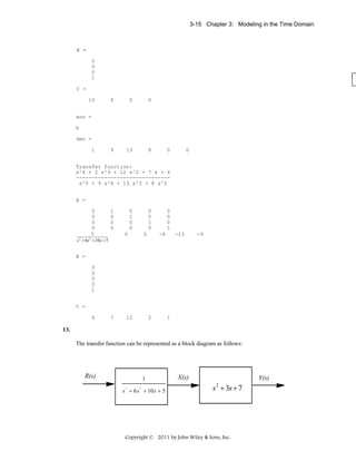
![F O U R
Time Response
SOLUTIONS TO CASE STUDIES CHALLENGES
Antenna Control: Open-Loop Response
The forward transfer function for angular velocity is,
ω0(s)
24
G(s) = V (s) = (s+150)(s+1.32)
P
a. ω0(t) = A + Be-150t + Ce-1.32t
24
b. G(s) = 2
. Therefore, 2ζωn =151.32, ωn = 14.07, and ζ = 5.38.
s +151.32s+198
24
c. ω0(s) =
2+151.32s+198) =
s(s
Therefore, ω0(t) = 0.12121 + .0010761 e-150t - 0.12229e-1.32t.
d. Using G(s),
••
•
ω 0 + 151.32 ω 0 + 198ω 0 = 24v p (t)
Defining,
x1 = ω 0
•
x2 = ω 0
Thus, the state equations are,
•
x1 = x 2
•
x2 = −198x1 − 151.32x2 + 24v p (t)
y = x1
In vector-matrix form,
•
1 ⎤
⎡0⎤
⎡ 0
x=⎢
x + ⎢ ⎥ v p (t); y = [1 0 ]x
⎣ 24⎦
⎣−198 −151.32⎥
⎦
Copyright © 2011 by John Wiley & Sons, Inc.](https://image.slidesharecdn.com/solutionscontrolsystemsengineeringbynormannice6ed-130502172814-phpapp02-131105052456-phpapp01/85/Solutions-control-system-sengineering-by-normannice-6ed-130502172814-phpapp02-108-320.jpg)
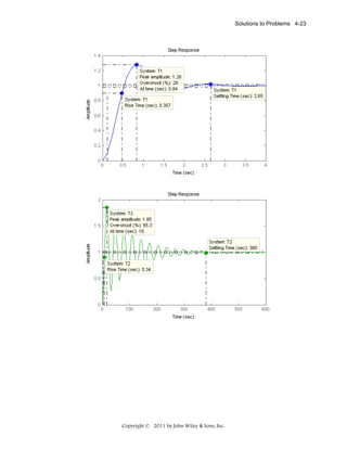
![4-2
Chapter 4: Time Response
e.
Program:
'Case Study 1 Challenge (e)'
num=24;
den=poly([-150 -1.32]);
G=tf(num,den)
step(G)
Computer response:
ans =
Case Study 1 Challenge (e)
Transfer function:
24
------------------s^2 + 151.3 s + 198
Ship at Sea: Open-Loop Response
a. Assuming a second-order approximation: ωn2 = 2.25, 2ζωn = 0.5. Therefore ζ = 0.167, ωn = 1.5.
Ts =
π
4
= 16; TP =
= 2.12 ;
ζωn
ωn 1-ζ2
%OS = e-ζπ /
1-ζ
2
x 100 = 58.8%; ωnTr = 1.169 therefore, Tr = 0.77.
s + 0.5
2.25
b. θ s =
= 1−
2 + 0.5 s + 2.25
2 + 0.5 s + 2.25
s s
s s
0.25
s + 0.25 +
2.1875
1−
2.1875
=
s
s + 0.25 2 + 2.1875
Copyright © 2011 by John Wiley & Sons, Inc.](https://image.slidesharecdn.com/solutionscontrolsystemsengineeringbynormannice6ed-130502172814-phpapp02-131105052456-phpapp01/85/Solutions-control-system-sengineering-by-normannice-6ed-130502172814-phpapp02-109-320.jpg)
![Answers to Review Questions 4-3
s + 0.25 + 0.16903 1.479
= 1−
s
s + 0.25 2 + 2.1875
Taking the inverse Laplace transform,
θ(t) = 1 - e-0.25t ( cos1.479t +0.16903 sin1.479t)
c.
Program:
'Case Study 2 Challenge (C)'
'(a)'
numg=2.25;
deng=[1 0.5 2.25];
G=tf(numg,deng)
omegan=sqrt(deng(3))
zeta=deng(2)/(2*omegan)
Ts=4/(zeta*omegan)
Tp=pi/(omegan*sqrt(1-zeta^2))
pos=exp(-zeta*pi/sqrt(1-zeta^2))*100
t=0:.1:2;
[y,t]=step(G,t);
Tlow=interp1(y,t,.1);
Thi=interp1(y,t,.9);
Tr=Thi-Tlow
'(b)'
numc=2.25*[1 2];
denc=conv(poly([0 -3.57]),[1 2 2.25]);
[K,p,k]=residue(numc,denc)
'(c)'
[y,t]=step(G);
plot(t,y)
title('Roll Angle Response')
xlabel('Time(seconds)')
ylabel('Roll Angle(radians)')
Computer response:
ans =
Case Study 2 Challenge (C)
ans =
(a)
Transfer function:
2.25
-----------------s^2 + 0.5 s + 2.25
omegan =
1.5000
zeta =
0.1667
Ts =
16
Copyright © 2011 by John Wiley & Sons, Inc.](https://image.slidesharecdn.com/solutionscontrolsystemsengineeringbynormannice6ed-130502172814-phpapp02-131105052456-phpapp01/85/Solutions-control-system-sengineering-by-normannice-6ed-130502172814-phpapp02-110-320.jpg)
![4-4
Chapter 4: Time Response
Tp =
2.1241
pos =
58.8001
Tr =
0.7801
ans =
(b)
K =
0.1260
-0.3431 + 0.1058i
-0.3431 - 0.1058i
0.5602
p =
-3.5700
-1.0000 + 1.1180i
-1.0000 - 1.1180i
0
k =
[]
ans =
(c)
Copyright © 2011 by John Wiley & Sons, Inc.](https://image.slidesharecdn.com/solutionscontrolsystemsengineeringbynormannice6ed-130502172814-phpapp02-131105052456-phpapp01/85/Solutions-control-system-sengineering-by-normannice-6ed-130502172814-phpapp02-111-320.jpg)
![4-8
Chapter 4: Time Response
3.
Program:
'(a)'
num=5;
den=[1 5];
Ga=tf(num,den)
subplot(1,2,1)
step(Ga)
title('(a)')
'(b)'
num=20;
den=[1 20];
Gb=tf(num,den)
subplot(1,2,2)
step(Gb)
title('(b)')
Computer response:
ans =
(a)
Transfer function:
5
----s + 5
ans =
(b)
Transfer function:
20
-----s + 20
Copyright © 2011 by John Wiley & Sons, Inc.](https://image.slidesharecdn.com/solutionscontrolsystemsengineeringbynormannice6ed-130502172814-phpapp02-131105052456-phpapp01/85/Solutions-control-system-sengineering-by-normannice-6ed-130502172814-phpapp02-115-320.jpg)
![Solutions to Problems 4-9
4.
VC(s)
1/ RC
0.703
5
. Since Vi(s) = s
Using voltage division, V (s) =
=
i
1
s + 0.703
S+
RC
5 ⎛ 0.703 ⎞ 5
5
Vc ( s ) = ⎜
.
⎟= −
s ⎝ s + 0.703 ⎠ s s + 0.703
Therefore vc (t ) = 5 − 5e
T=
−0.703t
. Also,
1
2.2
4
= 1.422; Tr =
= 3.129; Ts =
= 5.69 .
0.703
0.703
0.703
5.
Program:
clf
num=0.703;
den=[1 0.703];
G=tf(num,den)
step(5*G)
Computer response:
Transfer function:
0.703
--------s + 0.703
Copyright © 2011 by John Wiley & Sons, Inc.](https://image.slidesharecdn.com/solutionscontrolsystemsengineeringbynormannice6ed-130502172814-phpapp02-131105052456-phpapp01/85/Solutions-control-system-sengineering-by-normannice-6ed-130502172814-phpapp02-116-320.jpg)
![Solutions to Problems 4-11
7.
Program:
Clf
M=1
num=1/M;
den=[1 6/M];
G=tf(num,den)
step(G)
pause
M=2
num=1/M;
den=[1 6/M];
G=tf(num,den)
step(G)
Computer response:
M =
1
Transfer function:
1
----s + 6
M =
2
Transfer function:
0.5
----s + 3
Copyright © 2011 by John Wiley & Sons, Inc.](https://image.slidesharecdn.com/solutionscontrolsystemsengineeringbynormannice6ed-130502172814-phpapp02-131105052456-phpapp01/85/Solutions-control-system-sengineering-by-normannice-6ed-130502172814-phpapp02-118-320.jpg)
![Solutions to Problems 4-13
Tc
From plot, time constant = 0.33 s.
8.
a. Pole: -2; c(t) = A + Be-2t ; first-order response.
b. Poles: -3, -6; c(t) = A + Be-3t + Ce-6t; overdamped response.
c. Poles: -10, -20; Zero: -7; c(t) = A + Be-10t + Ce-20t; overdamped response.
d. Poles: (-3+j3 15 ), (-3-j3 15 ) ; c(t) = A + Be-3t cos (3 15 t + φ); underdamped.
e. Poles: j3, -j3; Zero: -2; c(t) = A + B cos (3t + φ); undamped.
f. Poles: -10, -10; Zero: -5; c(t) = A + Be-10t + Cte-10t; critically damped.
9.
Program:
p=roots([1 6 4 7 2])
Computer response:
p =
Copyright © 2011 by John Wiley & Sons, Inc.](https://image.slidesharecdn.com/solutionscontrolsystemsengineeringbynormannice6ed-130502172814-phpapp02-131105052456-phpapp01/85/Solutions-control-system-sengineering-by-normannice-6ed-130502172814-phpapp02-120-320.jpg)
![4-14
Chapter 4: Time Response
-5.4917
-0.0955 + 1.0671i
-0.0955 - 1.0671i
-0.3173
10.
G(s) = C (sI-A)-1 B
⎡ 8 −4 1 ⎤
⎡ −4 ⎤
⎢ −3 2 0 ⎥ ; B = ⎢ −3⎥ ; C = 2 8 −3
A=⎢
[
]
⎥
⎢ ⎥
⎢ 5 7 −9 ⎥
⎢4⎥
⎣
⎦
⎣ ⎦
( s − 2) ⎤
⎡ ( s − 2)( s + 9) −(4s + 29)
1
⎢ −(3s + 27) ( s 2 + s − 77)
⎥
( sI − A) −1 = 3 2
−3
⎢
⎥
s − s − 91s + 67
⎢ 5s − 31
7 s − 76
( s 2 − 10 s + 4) ⎥
⎣
⎦
Therefore, G(s ) =
−44 s 2 + 291s + 1814
.
s 3 − s 2 − 91s + 67
Factoring the denominator, or using det(sI-A), we find the poles to be 9.683, 0.7347, -9.4179.
11.
Program:
A=[8 -4 1;-3 2 0;5 7 -9]
B=[-4;-3;4]
C=[2 8 -3]
D=0
[numg,deng]=ss2tf(A,B,C,D,1);
G=tf(numg,deng)
poles=roots(deng)
Computer response:
A =
8
-4
1
-3
2
0
5
7
-9
B =
-4
-3
4
Copyright © 2011 by John Wiley & Sons, Inc.](https://image.slidesharecdn.com/solutionscontrolsystemsengineeringbynormannice6ed-130502172814-phpapp02-131105052456-phpapp01/85/Solutions-control-system-sengineering-by-normannice-6ed-130502172814-phpapp02-121-320.jpg)
![Solutions to Problems 4-15
C =
2
8
-3
D =
0
Transfer function:
-44 s^2 + 291 s + 1814
---------------------s^3 - s^2 - 91 s + 67
poles =
-9.4179
9.6832
0.7347
12.
VC(s) - V(s)
1
1
Writing the node equation at the capacitor, VC(s) (R + Ls + Cs) +
= 0.
R1
2
1
R1
VC(s)
10s
10
Hence, V(s) = 1
= 2
. The step response is 2
.The poles
1
1
s +20s+500
s +20s+500
+ R + Ls + Cs
R1
2
are at
-10 ± j20. Therefore, vC(t) = Ae-10t cos (20t + φ).
13.
Program:
num=[10 0];
den=[1 20 500];
G=tf(num,den)
step(G)
Computer response:
Transfer function:
10 s
---------------s^2 + 20 s + 500
Copyright © 2011 by John Wiley & Sons, Inc.](https://image.slidesharecdn.com/solutionscontrolsystemsengineeringbynormannice6ed-130502172814-phpapp02-131105052456-phpapp01/85/Solutions-control-system-sengineering-by-normannice-6ed-130502172814-phpapp02-122-320.jpg)
![Solutions to Problems 4-19
b. ωn2 = 0.04 r/s, 2ζωn = 0.02. Therefore ζ = 0.05, ωn = 0.2. Ts =
15.73 s; %OS = e-ζπ /
1-ζ
2
4
= 400 s; TP =
ζωn
ω
π
2
n 1-ζ
=
x 100 = 85.45 %; ωnTr = (1.76ζ3 - 0.417ζ2 + 1.039ζ + 1); therefore,
Tr = 5.26 s.
c. ωn2 = 1.05 x 10⁷ r/s, 2ζωn = 1.6 x 10³. Therefore ζ = 0.247, ωn = 3240. Ts =
π
ωn
1-ζ2
= 0.001 s; %OS = e-ζπ /
1-ζ
2
4
= 0.005 s; TP =
ζωn
x 100 = 44.92 %; ωnTr = (1.76ζ3 - 0.417ζ2 + 1.039ζ +
1); therefore, Tr = 3.88x10⁻⁴ s.
21.
Program:
'(a)'
clf
numa=16;
dena=[1 3 16];
Ta=tf(numa,dena)
omegana=sqrt(dena(3))
zetaa=dena(2)/(2*omegana)
Tsa=4/(zetaa*omegana)
Tpa=pi/(omegana*sqrt(1-zetaa^2))
Tra=(1.76*zetaa^3 - 0.417*zetaa^2 + 1.039*zetaa + 1)/omegana
percenta=exp(-zetaa*pi/sqrt(1-zetaa^2))*100
subplot(221)
step(Ta)
title('(a)')
'(b)'
numb=0.04;
denb=[1 0.02 0.04];
Tb=tf(numb,denb)
omeganb=sqrt(denb(3))
zetab=denb(2)/(2*omeganb)
Tsb=4/(zetab*omeganb)
Tpb=pi/(omeganb*sqrt(1-zetab^2))
Trb=(1.76*zetab^3 - 0.417*zetab^2 + 1.039*zetab + 1)/omeganb
percentb=exp(-zetab*pi/sqrt(1-zetab^2))*100
subplot(222)
step(Tb)
title('(b)')
'(c)'
numc=1.05E7;
denc=[1 1.6E3 1.05E7];
Tc=tf(numc,denc)
omeganc=sqrt(denc(3))
zetac=denc(2)/(2*omeganc)
Tsc=4/(zetac*omeganc)
Tpc=pi/(omeganc*sqrt(1-zetac^2))
Trc=(1.76*zetac^3 - 0.417*zetac^2 + 1.039*zetac + 1)/omeganc
percentc=exp(-zetac*pi/sqrt(1-zetac^2))*100
subplot(223)
step(Tc)
title('(c)')
Copyright © 2011 by John Wiley & Sons, Inc.](https://image.slidesharecdn.com/solutionscontrolsystemsengineeringbynormannice6ed-130502172814-phpapp02-131105052456-phpapp01/85/Solutions-control-system-sengineering-by-normannice-6ed-130502172814-phpapp02-126-320.jpg)
![4-22
Chapter 4: Time Response
22.
Program:
T1=tf(16,[1 3 16])
T2=tf(0.04,[1 0.02 0.04])
T3=tf(1.05e7,[1 1.6e3 1.05e7])
ltiview
Computer response:
Transfer function:
16
-------------s^2 + 3 s + 16
Transfer function:
0.04
------------------s^2 + 0.02 s + 0.04
Transfer function:
1.05e007
----------------------s^2 + 1600 s + 1.05e007
Copyright © 2011 by John Wiley & Sons, Inc.](https://image.slidesharecdn.com/solutionscontrolsystemsengineeringbynormannice6ed-130502172814-phpapp02-131105052456-phpapp01/85/Solutions-control-system-sengineering-by-normannice-6ed-130502172814-phpapp02-129-320.jpg)
![Solutions to Problems 4-29
Since the amplitude of the sinusoids are of two orders of magnitude larger than the residue of the pole
at -2, pole-zero cancellation can be assumed. Since 2ζωn = 1, and ωn = 5 = 2.236, ζ = 0.224,
%OS = e
−ζπ / 1−ζ
2
π
4
x100 = 48.64% , Ts = ζω = 8 sec, Tp =
n
ωn 1-ζ2
= 1.44 sec; ωnTr = 1.23,
therefore, Tr = 0.55.
d.
Since the amplitude of the sinusoids are of two orders of magnitude larger than the residue of the pole
at -2, pole-zero cancellation can be assumed. Since 2ζωn = 5, and ωn = 20 = 4.472, ζ = 0.559,
%OS = e
−ζπ / 1−ζ
2
4
x100 = 12.03% , Ts = ζω = 1.6 sec, Tp =
n
1.852, therefore, Tr = 0.414.
31.
Program:
%Form sC(s) to get transfer function
clf
num=[1 3];
den=conv([1 3 10],[1 2]);
T=tf(num,den)
step(T)
Computer response:
Transfer function:
s + 3
----------------------s^3 + 5 s^2 + 16 s + 20
Copyright © 2011 by John Wiley & Sons, Inc.
π
ωn 1-ζ2
= 0.847 sec; ωnTr =](https://image.slidesharecdn.com/solutionscontrolsystemsengineeringbynormannice6ed-130502172814-phpapp02-131105052456-phpapp01/85/Solutions-control-system-sengineering-by-normannice-6ed-130502172814-phpapp02-136-320.jpg)
![Solutions to Problems 4-35
36.
a.
−2
−3 ⎤
⎡ 1 0 0⎤ ⎡0 2 3 ⎤ ⎡ s
−5 ⎥
sI − A = s ⎢ 0 1 0⎥ − ⎢0 6 5 ⎥ = ⎢ 0 (s − 6)
⎢ 0 0 1⎥ ⎢1 4 2 ⎥ ⎢ −1
−4
(s − 2)⎥
⎦ ⎣
⎦
⎦ ⎣
⎣
sI − A = s 3 − 8s 2 − 11s + 8
b. Factoring yields poles at 9.111, 0.5338, and –1.6448.
37.
x = (sI - A ) -1 (x0 + B u )
−1
⎛ ⎡1 0 ⎤ ⎡1
2 ⎤ ⎞ ⎛ ⎡3⎤ ⎡1⎤
1 ⎞
X = ⎜s⎢
⎥ − ⎢ −3 −1⎥ ⎟ ⎜ ⎢1⎥ + ⎢1⎥ ⋅ 3 s 2 + 9 ⎟
⎦⎠ ⎝⎣ ⎦ ⎣ ⎦
⎝ ⎣0 1 ⎦ ⎣
⎠
⎛ 3s 3 + 5s 2 + 30 s + 54 ⎞
⎜
⎟
[ s 2 + 5][ s 2 + 9] ⎟
X =⎜ 3
⎜ s − 10s 2 + 12 s − 102 ⎟
⎜
⎜ [ s 2 + 5][ s 2 + 9] ⎟
⎟
⎝
⎠
Y ( s ) = [1 2] X
⎛ 5s 3 − 15s 2 + 54 s − 150 ⎞
Y (s) = ⎜
⎟
[ s 2 + 9][ s 2 + 5]
⎝
⎠
38.
x = (sI - A ) -1 (x0 + B u )
Y ( s ) = [0 0 1]X
Y (s) =
s 2 + 4s + 2
[ s + 6][ s + 1][ s + 0.58579][ s + 3.4142]
Copyright © 2011 by John Wiley & Sons, Inc.](https://image.slidesharecdn.com/solutionscontrolsystemsengineeringbynormannice6ed-130502172814-phpapp02-131105052456-phpapp01/85/Solutions-control-system-sengineering-by-normannice-6ed-130502172814-phpapp02-142-320.jpg)
![4-36
Chapter 4: Time Response
39.
x = (sI - A ) -1 (x0 + B u )
−1
⎛ ⎡1 0 ⎤ ⎡ −2 0 ⎤ ⎞ ⎛ ⎡ 3⎤ ⎡1⎤ 1 ⎞
X = ⎜s⎢
⎥−⎢
⎥⎟ ⎜⎢ ⎥ + ⎢ ⎥ ⎟
⎝ ⎣0 1 ⎦ ⎣ −1 −1⎦ ⎠ ⎝ ⎣0 ⎦ ⎣1⎦ s ⎠
3s + 1
⎛
⎞
⎜ s[ s + 2] ⎟
⎟
X =⎜
1 − 2s
⎜
⎟
⎜ s[ s + 1][ s + 2] ⎟
⎝
⎠
Y ( s ) = [0 1]X
⎛
⎞
1 − 2s
Y (s) = ⎜
⎟
⎝ s[ s + 1][ s + 2] ⎠
Applying partial fraction decomposition,
3
5 1 ⎞
⎛11
Y (s) = ⎜
−
+
⎟
⎝ 2 s s +1 2 s + 2 ⎠
1
5
y (t ) = u (t ) − 3e− t + e−2t
2
2
40.
−1
x = (sI − A) (x 0 + Bu)
⎛ ⎡1 0
x = ⎜ s⎢0 1
⎜
⎝ ⎢0 0
⎣
0⎤ ⎡ −3 1
0 ⎤⎞
0⎥ − ⎢ 0 −6 1 ⎥ ⎟
⎟
1⎥ ⎢ 0
0 −5⎥ ⎠
⎦ ⎣
⎦
−1
⎛ ⎡ 0⎤ ⎡ 0⎤ ⎞
⎜ ⎢ 0⎥ + ⎢ 1⎥ 1 ⎟
⎜
s⎟
⎝ ⎢ 0⎥ ⎢ 1⎥ ⎠
⎣ ⎦ ⎣ ⎦
⎤
1
⎡
⎢ s(s + 3)(s + 5) ⎥
1
⎥
x=⎢
⎢ s(s + 5) ⎥
1
⎢
⎥
⎣ s(s + 5) ⎦
⎡ 1 − 1 e −3 t + 1 e −5 t ⎤
10
⎥
⎢ 15 6
1 1 −5 t
⎥
x (t) = ⎢
− e
5 5
⎢
⎥
1 1 −5 t
− e
⎢
⎥
⎣
⎦
5 5
Copyright © 2011 by John Wiley & Sons, Inc.](https://image.slidesharecdn.com/solutionscontrolsystemsengineeringbynormannice6ed-130502172814-phpapp02-131105052456-phpapp01/85/Solutions-control-system-sengineering-by-normannice-6ed-130502172814-phpapp02-143-320.jpg)
![Solutions to Problems 4-37
y(t ) = [0 1 1]x =
2 2 −5t
− e
5 5
41.
Program:
A=[-3 1 0;0 -6 1;0 0 -5];
B=[0;1;1];
C=[0 1 1];
D=0;
S=ss(A,B,C,D)
step(S)
Computer response:
a =
x1
x2
x3
x1
-3
0
0
x2
1
-6
0
x3
0
1
-5
x2
1
x3
1
b =
x1
x2
x3
u1
0
1
1
c =
y1
x1
0
d =
y1
u1
0
Continuous-time model.
Copyright © 2011 by John Wiley & Sons, Inc.](https://image.slidesharecdn.com/solutionscontrolsystemsengineeringbynormannice6ed-130502172814-phpapp02-131105052456-phpapp01/85/Solutions-control-system-sengineering-by-normannice-6ed-130502172814-phpapp02-144-320.jpg)
![4-38
Chapter 4: Time Response
42.
Program:
syms s
'a'
A=[-3 1 0;0 -6 1;0 0 -5]
B=[0;1;1];
C=[0 1 1];
X0=[1;1;0]
U=1/s;
I=[1 0 0;0 1 0;0 0 1];
X=((s*I-A)^-1)*(X0+B*U);
x1=ilaplace(X(1))
x2=ilaplace(X(2))
x3=ilaplace(X(3))
y=C*[x1;x2;x3]
y=simplify(y)
'y(t)'
pretty(y)
%Construct symbolic object for
%frequency variable 's'.
%Display label
%Create matrix A.
%Create vector B.
%Create C vector
%Create initial condition vector,X(0).
%Create U(s).
%Create identity matrix.
%Find Laplace transform of state vector.
%Solve for X1(t).
%Solve for X2(t).
%Solve for X3(t).
%Solve for output, y(t).
%Simplify y(t).
%Display label.
%Pretty print y(t).
Computer response:
ans =
a
A =
-3
0
0
1
-6
0
0
1
-5
X0 =
1
1
0
x1 =
7/6*exp(-3*t)-1/3*exp(-6*t)+1/15+1/10*exp(-5*t)
x2 =
exp(-6*t)+1/5-1/5*exp(-5*t)
x3 =
1/5-1/5*exp(-5*t)
y =
2/5+exp(-6*t)-2/5*exp(-5*t)
y =
2/5+exp(-6*t)-2/5*exp(-5*t)
ans =
y(t)
2/5 + exp(-6 t) - 2/5 exp(-5 t)
43.
|λI - A | = λ2 + 5λ +1
|λI - A | = (λ + 0.20871) (λ + 4.7913)
Copyright © 2011 by John Wiley & Sons, Inc.](https://image.slidesharecdn.com/solutionscontrolsystemsengineeringbynormannice6ed-130502172814-phpapp02-131105052456-phpapp01/85/Solutions-control-system-sengineering-by-normannice-6ed-130502172814-phpapp02-145-320.jpg)
![4-40
Chapter 4: Time Response
Solving for the Ai's and substituting into the state-transition matrix,
To find the state vector,
y = (3, 4) x
⎛ 1 − cos[t ] ⎞
Δy = (3, 4) ⎜
⎟
⎝ sin[t ] ⎠
y = (−3cos[t ] + 4sin[t ] + 3)
45.
|λI - A | = (λ + 2) (λ + 0.5 - 2.3979i) (λ + 0.5 + 2.3979i)
Let the state-transition matrix be
Copyright © 2011 by John Wiley & Sons, Inc.](https://image.slidesharecdn.com/solutionscontrolsystemsengineeringbynormannice6ed-130502172814-phpapp02-131105052456-phpapp01/85/Solutions-control-system-sengineering-by-normannice-6ed-130502172814-phpapp02-147-320.jpg)
![Solutions to Problems 4-41
.
..
Since φ(0) = I, Φ(0) = A, and φ(0) = A2, we can evaluate the coefficients, Ai's. Thus,
Solving for the Ai's taking three equations at a time,
t
U s i n g x (t ) = φ (t )x (0 ) + ∫ φ (t -τ )B u (τ )dτ , a n d y =
1
0
0
0
1 1
= 2 - 2 e-2t
46.
Program:
syms s t tau
'a'
A=[-2 1 0;0 0 1;0 -6 -1]
B=[1;0;0]
C=[1 0 0]
X0=[1;1;0]
I=[1 0 0;0 1 0;0 0 1];
'E=(s*I-A)^-1'
E=((s*I-A)^-1)
Fi11=ilaplace(E(1,1));
Fi12=ilaplace(E(1,2));
Fi13=ilaplace(E(1,3));
Fi21=ilaplace(E(2,1));
Fi22=ilaplace(E(2,2));
Fi23=ilaplace(E(2,3));
%Construct symbolic object for
%frequency variable 's', 't', and 'tau.
%Display label.
%Create matrix A.
%Create vector B.
%Create vector C.
%Create initial condition vector,X(0).
%Create identity matrix.
%Display label.
%Find Laplace transform of state
%transition matrix, (sI-A)^-1.
%Take inverse Laplace transform
%of each element
Copyright © 2011 by John Wiley & Sons, Inc.
x (t ),](https://image.slidesharecdn.com/solutionscontrolsystemsengineeringbynormannice6ed-130502172814-phpapp02-131105052456-phpapp01/85/Solutions-control-system-sengineering-by-normannice-6ed-130502172814-phpapp02-148-320.jpg)
![4-42
Chapter 4: Time Response
Fi31=ilaplace(E(3,1));
Fi32=ilaplace(E(3,2));
%to find state transition matrix.
Fi33=ilaplace(E(3,3));
%of (sI-A)^-1.
'Fi(t)'
%Display label.
Fi=[Fi11 Fi12 Fi13
%Form Fi(t).
Fi21 Fi22 Fi23
Fi31 Fi32 Fi33];
pretty(Fi)
%Pretty print state transition matrix, Fi.
Fitmtau=subs(Fi,t,t-tau);
%Form Fi(t-tau).
'Fi(t-tau)'
%Display label.
pretty(Fitmtau)
%Pretty print Fi(t-tau).
x=Fi*X0+int(Fitmtau*B*1,tau,0,t);
%Solve for x(t).
x=simple(x);
%Collect terms.
x=simplify(x);
%Simplify x(t).
x=vpa(x,3);
'x(t)'
%Display label.
pretty(x)
%Pretty print x(t).
y=C*x;
%Find y(t)
y=simplify(y);
y=vpa(simple(y),3);
y=collect(y);
'y(t)'
pretty(y)
%Pretty print y(t).
Computer response:
ans =
a
A =
-2
0
0
1
0
-6
0
1
-1
0
0
B =
1
0
0
C =
1
X0 =
1
1
0
ans =
E=(s*I-A)^-1
E =
[
[
[
1/(s+2), (s+1)/(s+2)/(s^2+s+6),
0,
(s+1)/(s^2+s+6),
0,
-6/(s^2+s+6),
1/(s+2)/(s^2+s+6)]
1/(s^2+s+6)]
s/(s^2+s+6)]
Copyright © 2011 by John Wiley & Sons, Inc.](https://image.slidesharecdn.com/solutionscontrolsystemsengineeringbynormannice6ed-130502172814-phpapp02-131105052456-phpapp01/85/Solutions-control-system-sengineering-by-normannice-6ed-130502172814-phpapp02-149-320.jpg)
![Solutions to Problems 4-43
ans =
Fi(t)
[
13
[exp(-2 t) , - 1/8 exp(-2 t) + 1/8 %1 + --- %2 ,
[
184
]
1/8 exp(-2 t) - 1/8 %1 + 3/184 %2]
]
[
[0 , 1/23 %2 + %1 , - 1/23
1/2
1/2
1/2
(-23)
(exp((-1/2 + 1/2 (-23)
) t) - exp((-1/2 - 1/2 (-23)
) t))
]
]
[
[0 , 6/23
1/2
1/2
1/2
(-23)
(exp((-1/2 + 1/2 (-23)
) t) - exp((-1/2 - 1/2 (-23)
) t))
]
, - 1/23 %2 + %1]
1/2
%1 := exp(- 1/2 t) cos(1/2 23
t)
1/2
1/2
%2 := exp(- 1/2 t) 23
sin(1/2 23
t)
ans =
Fi(t-tau)
[
[exp(-2 t + 2 tau) ,
[
13
1/2
- 1/8 exp(-2 t + 2 tau) + 1/8 %2 cos(%1) + --- %2 23
sin(%1) ,
184
1/2
]
1/8 exp(-2 t + 2 tau) - 1/8 %2 cos(%1) + 3/184 %2 23
sin(%1)]
]
[
1/2
1/2
[0 , 1/23 %2 23
sin(%1) + %2 cos(%1) , - 1/23 (-23)
(
1/2
exp((-1/2 + 1/2 (-23)
) (t - tau))
1/2
]
- exp((-1/2 - 1/2 (-23)
) (t - tau)))]
[
1/2
1/2
[0 , 6/23 (-23)
(exp((-1/2 + 1/2 (-23)
) (t - tau))
1/2
- exp((-1/2 - 1/2 (-23)
) (t - tau))) ,
Copyright © 2011 by John Wiley & Sons, Inc.](https://image.slidesharecdn.com/solutionscontrolsystemsengineeringbynormannice6ed-130502172814-phpapp02-131105052456-phpapp01/85/Solutions-control-system-sengineering-by-normannice-6ed-130502172814-phpapp02-150-320.jpg)
![4-44
Chapter 4: Time Response
1/2
]
- 1/23 %2 23
sin(%1) + %2 cos(%1)]
1/2
%1 := 1/2 23
(t - tau)
%2 := exp(- 1/2 t + 1/2 tau)
ans =
x(t)
[.375 exp(-2. t) + .125 exp(-.500 t) cos(2.40 t)
+ .339 exp(-.500 t) sin(2.40 t) + .500]
[.209 exp(-.500 t) sin(2.40 t) + exp(-.500 t) cos(2.40 t)]
[1.25 i (exp((-.500 + 2.40 i) t) - 1. exp((-.500 - 2.40 i) t))]
ans =
y(t)
.375 exp(-2. t) + .125 exp(-.500 t) cos(2.40 t)
+ .339 exp(-.500 t) sin(2.40 t) + .500
47.
The state-space representation used to obtain the plot is,
.
x =
0
-1
1
-0.8
x +
0
1
u(t); y(t) =
1
Using the Step Response software,
Copyright © 2011 by John Wiley & Sons, Inc.
0
x](https://image.slidesharecdn.com/solutionscontrolsystemsengineeringbynormannice6ed-130502172814-phpapp02-131105052456-phpapp01/85/Solutions-control-system-sengineering-by-normannice-6ed-130502172814-phpapp02-151-320.jpg)
![4-46
Chapter 4: Time Response
49.
s+0.5
1/20
1/4 3/10
1
1
3
a. P(s) = s(s+2)(s+5) = s + s+2 - s+5 . Therefore, p(t) = 20 + 4 e-2t - 10 e-5t.
b. To represent the system in state space, draw the following block diagram.
V(s)
Y(s)
1
s +7s+10
For the first block,
..
P(s)
s+0.5
2
.
y + 7y + 10y = v(t)
.
Let x1 = y, and x2 = y . Therefore,
.
x 1 = x2
.
x 2 = -10x1 - 7x2 + v(t)
Also,
.
p(t) = 0.5y + y = 0.5x1 + x2
Thus,
.
x =
0
-1 0
1
-7
x +
0
1
1 ; p (t ) =
0.5
c.
Program:
A=[0 1;-10 -7];
B=[0;1];
C=[.5 1];
D=0;
S=ss(A,B,C,D)
step(S)
Copyright © 2011 by John Wiley & Sons, Inc.
1
x](https://image.slidesharecdn.com/solutionscontrolsystemsengineeringbynormannice6ed-130502172814-phpapp02-131105052456-phpapp01/85/Solutions-control-system-sengineering-by-normannice-6ed-130502172814-phpapp02-153-320.jpg)
![4-48
Chapter 4: Time Response
b. Ge(s) =
K
K
=
. Representing the system in phase-variable form:
(s+10)(s2+4s+10) s3+14s2+50s+100
1
0 ⎤
⎡ 0
⎡0⎤
A=⎢ 0
0
1 ⎥; B = ⎢ 0 ⎥; C = [1 0 0 ]
⎢ −100 −50 −14⎥
⎢K ⎥
⎣
⎦
⎣ ⎦
c.
Program:
numg=100;
deng=conv([1 10],[1 4 10]);
G=tf(numg,deng)
step(G)
Computer response:
Transfer function:
100
------------------------s^3 + 14 s^2 + 50 s + 100
%OS =
(1.08-1)
* 100 = 8%
1
Copyright © 2011 by John Wiley & Sons, Inc.](https://image.slidesharecdn.com/solutionscontrolsystemsengineeringbynormannice6ed-130502172814-phpapp02-131105052456-phpapp01/85/Solutions-control-system-sengineering-by-normannice-6ed-130502172814-phpapp02-155-320.jpg)
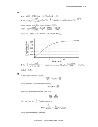
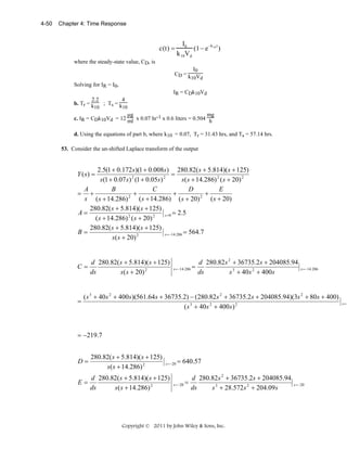
![Solutions to Problems 4-51
=
( s 3 + 28.572s 2 + 204.09 s)(561.64 s + 36735.2) − (280.82s 2 + 36735.2 s + 204085.94)(3s 2 + 57.144s + 204.09)
( s 3 + 28.572 s 2 + 204.09 s ) 2
= 217.18
thus
Y (s) =
2.5
564.7
219.7
640.57
217.18
+
−
+
+
2
2
s
( s + 14.286) ( s + 20)
( s + 20)
( s + 14.286)
Obtaining the inverse Laplace transform of the latter and delaying the equation in time domain we
get
y (t ) = [2.5 + 564.7(t − 0.008)e −14.286 (t −0.008) − 219.7e −14.286 ( t −0.008) + 640.57(t − 0.008)e −20 ( t −0.008)
+ 217.18e − 20 (t −0.008) ]u (t − 0.008)
54.
a. The transfer function can be written as
θ
I
(s) =
2.5056( s + 3.33)e −0.1s
( s + 1)( s 2 + 0.72s + 1.44)
It has poles at s=-0.36±j1.145 and s=-1. A zero at s=-3.33
The ‘far away’ pole at -1 is relatively close to the complex conjugate poles as 0.36*5>1 so a
dominant pole approximation can’t be applied.
b) In time domain the input can be expressed as:
i (t ) = 250μA(u (t ) − u (t − 0.15))
Obtaining Laplace transforms this can be expressed as
Copyright © 2011 by John Wiley & Sons, Inc.
s = −20](https://image.slidesharecdn.com/solutionscontrolsystemsengineeringbynormannice6ed-130502172814-phpapp02-131105052456-phpapp01/85/Solutions-control-system-sengineering-by-normannice-6ed-130502172814-phpapp02-158-320.jpg)
![Solutions to Problems 4-53
5.8 3.4 2.4( s + 0.15) + 4.768 5.8 3.4
2.4( s + 0.15)
−
−
=
−
−
2
s s + 1 ( s + 0.36) + 1.3104
s s + 1 ( s + 0.36) 2 + 1.3104
1.145
−4.164
( s + 0.36) 2 + 1.3104
=
Obtaining inverse Laplace transform we get
θ (t ) = 5.8 − 3.4e −t − 2.4e −0.36t cos(1.145t ) − 4.164e −0.36t sin(1.145t )
= 5.8 − 3.4e − t − 2.4e −0.36t sin(1.145t + 30 o )
So the actual (shifted) unit step response is given by
θ (t ) = [5.8 − 3.4e − (t −0.1) − 2.4e −0.36 (t −0.1) sin(1.145(t − 0.1) + 30 o )]u (t − 0.1)
The response to the pulse is given by:
θ (t ) = [1.45m − 0.85me − (t −0.1) − 0.6me −0.36 (t −0.1) sin(1.145(t − 0.1) + 30 o )]u (t − 0.1) −
[1.45m − 0.85me − ( t −0.25) − 0.6me −0.36 (t −0.25) sin(1.145(t − 0.25) + 30 o )]u (t − 0.25)
55.
At steady state the input is ≈ 9V and the output is ≈ 6V Thus G(0)=6/9=0.667
The maximum peak is achieved at ≈ 285μ with a %OS = (7.5/6-1)*100 = 25%
This corresponds to a damping factor of
ζ =
− ln(%OS / 100)
=
1.3863
≈ 0.4
π 2 + ln 2 (%OS / 100)
π 2 + 1.9218
π
π
ωn =
=
= 12027.2
2
(285μ )(0.9165)
Tp 1 − ζ
So the approximated transfer function is
Copyright © 2011 by John Wiley & Sons, Inc.](https://image.slidesharecdn.com/solutionscontrolsystemsengineeringbynormannice6ed-130502172814-phpapp02-131105052456-phpapp01/85/Solutions-control-system-sengineering-by-normannice-6ed-130502172814-phpapp02-160-320.jpg)
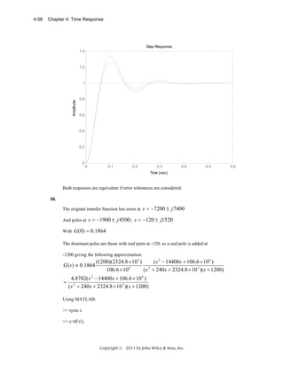
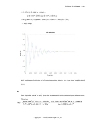
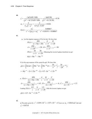
![4-60
Chapter 4: Time Response
63.
a.
Program
numg=[33 202 10061 24332 170704];
deng=[1 8 464 2411 52899 167829 913599 1076555];
G=tf(numg,deng)
[K,p,k]=residue(numg,deng)
Computer Response
K =
0.0018
0.0018
-0.1155
-0.1155
0.0077
0.0077
0.2119
+
+
+
0.0020i
0.0020i
0.0062i
0.0062i
0.0108i
0.0108i
p =
-1.6971
-1.6971
-0.5992
-0.5992
-1.0117
-1.0117
-1.3839
+16.4799i
-16.4799i
+12.1443i
-12.1443i
+ 4.2600i
- 4.2600i
k =
[]
b.
Therefore, an approximation to G(s)/ is:
G ( s) =
0.2119
s + 1.3839
c.
Program
numg=[33 202 10061 24332 170704];
deng=[1 8 464 2411 52899 167829 913599 1076555];
G=tf(numg,deng);
numga=0.2119;
denga=[1 1.3839];
Copyright © 2011 by John Wiley & Sons, Inc.](https://image.slidesharecdn.com/solutionscontrolsystemsengineeringbynormannice6ed-130502172814-phpapp02-131105052456-phpapp01/85/Solutions-control-system-sengineering-by-normannice-6ed-130502172814-phpapp02-167-320.jpg)
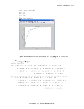
![4-62
Chapter 4: Time Response
65.
a. To find the step responses for these two processes, ya(t) and yp(t), we consider first the un-shifted
Laplace transform of their outputs for Xa(s) = Xp(s) = 1/s:
Ya* ( s) =
14.49
9.8 × 10 −3
A
B
(1),
=
= +
−4
s (1478.26 s + 1) s( s + 6.77 × 10 ) s ( s + 6.77 × 10 − 4 )
9.8 × 10 −3
= 14.49 and
s + 6.77 × 10 − 4 s = 0
9.8 × 10 −3
B=
= − 14.49 (2)
s
−4
s = −6.77 × 10
where A =
Substituting the values of A and B into equation (1) gives:
Ya* ( s ) =
⎛1
⎞
A
B
1
+
= 14.49 ⎜ −
−4
⎜ s ( s + 6.76 × 10 − 4 ) ⎟ (3)
⎟
s ( s + 6.76 × 10 )
⎝
⎠
*
Taking the inverse Laplace transform of Ya ( s ) and delaying the resulting response in the time
domain by 4 seconds, we get:
y a (t ) = 14.49[1 − e
− 6.76 × 10 −4 (t − 4)
Copyright © 2011 by John Wiley & Sons, Inc.
] u (t − 4) (4)](https://image.slidesharecdn.com/solutionscontrolsystemsengineeringbynormannice6ed-130502172814-phpapp02-131105052456-phpapp01/85/Solutions-control-system-sengineering-by-normannice-6ed-130502172814-phpapp02-169-320.jpg)
![Solutions to Problems 4-63
Noting that the denominator of G p (s ) can be factored into
( s + 0.174 × 10 −3 )(s + 6.814 × 10 −3 ) , we have:
*
Y p (s) =
1.716 ×10 −5
s ( s + 0.174 ×10 − 3 )( s + 6.814 ×10 − 3 )
where:
C=
=
C
D
E
(5),
+
+
s ( s + 0.174 ×10 − 3 ) ( s + 6.814 ×10 − 3 )
1.716 × 10 −5
( s + 0.174 × 10 − 3 )( s + 6.814 × 10 − 3 ) s = 0
D=
E=
1.716 × 10 −5
s ( s + 6.814 × 10 − 3 ) s = − 0.174 × 10 − 3
1.716 × 10 −5
s ( s + 0.174 × 10 − 3 ) s = −6.814 × 10 − 3
= 14.48 ;
= −14.85 ;
= 0.37 . (6)
Substituting the values of C, D and E into equation (5) and simplifying gives:
*
Y p ( s) =
⎛1
⎞
14.48
14.85
0.37
1.0256
0.0256
⎟ (7)
−
+
= 14.48 ⎜ −
+
⎜ s ( s + 0.174 × 10 − 3 ) ( s + 6.814 × 10 − 3 ) ⎟
s
( s + 0.174 × 10 − 3 ) ( s + 6.814 × 10 − 3 )
⎝
⎠
*
Taking the inverse Laplace transform of Y p ( s ) and delaying the resulting response in the time
domain by 30 seconds, we get:
y p (t ) = 14.48[1 − 1.0256 e
− 0.174 ×10 −3 (t − 30)
+ 0.0256 e
− 6.814 × 10 −3 (t − 30)
] u (t − 30) (8)
b. Using Simulink to model the two processes described above, ya(t) and yp(t) were output to the
“workspace.” Matlab plot commands were then utilized to plot ya(t) and yp(t) on a single graph,
which is shown below.
Copyright © 2011 by John Wiley & Sons, Inc.](https://image.slidesharecdn.com/solutionscontrolsystemsengineeringbynormannice6ed-130502172814-phpapp02-131105052456-phpapp01/85/Solutions-control-system-sengineering-by-normannice-6ed-130502172814-phpapp02-170-320.jpg)
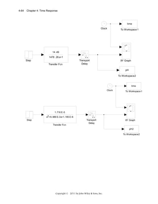
![4-66
Chapter 4: Time Response
66.
a.
>> A=[-8.792e-3 0.56e-3 -1e-3 -13.79e-3; -0.347e-3 -11.7e-3 -0.347e-3 0; 0.261 -20.8e-3 -96.6e-3
0; 0 0 1 0]
A=
-0.0088
0.0006 -0.0010 -0.0138
-0.0003 -0.0117 -0.0003
0
0.2610 -0.0208 -0.0966
0
0
0
1.0000
0
>> eig(A)
ans =
-0.1947
0.0447 + 0.1284i
0.0447 - 0.1284i
-0.0117
b.
Given the eigenvalues, the state-transition matrix will be of the form
⎡ K 11
⎢K
Φ(t ) = ⎢ 21
⎢ K 31
⎢
⎣ K 41
K 12
K 22
K 13
K 23
K 32
K 42
K 33
K 43
K 14 ⎤
K 24 ⎥
⎥
K 34 ⎥
⎥
K 44 ⎦
with
K ij = K ij 1 e − 0 .1947 t + K ij 2 e − 0 .0117 t + K ij 3 e + 0 .0447 t sin( 0 . 1284 t ) + K ij 4 e + 0 .0447 t cos( 0 . 1284 t ))
Thus 64 constants have to be found.
Copyright © 2011 by John Wiley & Sons, Inc.](https://image.slidesharecdn.com/solutionscontrolsystemsengineeringbynormannice6ed-130502172814-phpapp02-131105052456-phpapp01/85/Solutions-control-system-sengineering-by-normannice-6ed-130502172814-phpapp02-173-320.jpg)
![Solutions to Problems 4-67
67.
a. The equations are rewritten as
di L
1− d
1
=−
uC + E s
dt
L
L
du C 1 − d
1
=
iL −
uC
dt
C
RC
from which we obtain
⎡ di L ⎤ ⎡
⎢ dt ⎥ ⎢ 0
⎢ du ⎥ = ⎢1 − d
⎢ C⎥ ⎢
⎣ dt ⎦ ⎣ C
⎡i ⎤
y = [0 1]⎢ L ⎥
⎣iC ⎦
1− d ⎤
⎡1⎤
L ⎥ ⎡ iL ⎤ + ⎢ ⎥ E
1 ⎥ ⎢u C ⎥ ⎢ L ⎥ s
⎥⎣ ⎦ ⎣ 0 ⎦
−
RC ⎦
−
b. To obtain the transfer function we first calculate
( sI − A) −1
⎡
⎢ s
=⎢
1− d
⎢−
⎣ C
1− d ⎤
L ⎥
1 ⎥
⎥
s+
RC ⎦
−1
1
1− d ⎤
⎡
⎢ s + RC − L ⎥
⎢ 1− d
⎥
⎢
s ⎥
C
⎦
= ⎣
1
(1 − d ) 2
s(s +
)+
RC
LC
So
1
1− d ⎤
⎡
⎢ s + RC − L ⎥
⎢ 1− d
⎥
⎢
s ⎥ ⎡1⎤
C
⎦ ⎢ ⎥
G ( s ) = C( sI − A) −1 B = [0 1] ⎣
L
1
(1 − d ) 2 ⎢ 0 ⎥
⎣ ⎦
s( s +
)+
RC
LC
⎡1 − d
⎤
1− d
s⎥
⎡1⎤
⎢ C
⎣
⎦
LC
⎢L⎥ =
=
1
(1 − d ) 2
1
(1 − d ) 2 ⎢ 0 ⎥
⎣ ⎦ s2 +
s2 +
s+
s+
RC
RC
LC
LC
Copyright © 2011 by John Wiley & Sons, Inc.](https://image.slidesharecdn.com/solutionscontrolsystemsengineeringbynormannice6ed-130502172814-phpapp02-131105052456-phpapp01/85/Solutions-control-system-sengineering-by-normannice-6ed-130502172814-phpapp02-174-320.jpg)
![Solutions to Problems 4-69
b.
⎡− 0.036e −0.28t + 1.04e −8.06t ⎤
Φ(t )B = ⎢
⎥
− 0.28t
− 0.129e −8.06t ⎦
⎣ 0.129e
CΦ(t )B = −0.451e −0.28t + 13.04e −8.06t + 0.292e −0.28t − 0.292e −8.06t = −0.159e −0.28t + 12.748e −8.06t
Since u (t ) = 1
t
t
y (t ) = ∫ CΦ(t − τ )Bdτ = ∫ [−0.159e −0.28( t −τ ) + 12.748e −8.06 ( t −τ ) ]dτ
0
0
t
t
0
0
= −0.159e −0.28t ∫ e 0.28τ dτ + 12.748e −8.06t ∫ e 8.06τ dτ
=
− 0.159 −0.28t 0.28τ 12.748 −8.06t 8.06τ
e
e
+
e
e
0.28
8.06
t
0
= −0.568[1 − e −0.28t ] + 1.582[1 − e −8.06t ] = 1.014 + 0.568e −0.28t − 1.582e −8.06t
c.
>> A=[-8.34 -2.26; 1 0];
>> B = [1; 0];
>> C = [12.54 2.26];
>> D = 0;
>> t = linspace(0,15,1000);
>> y1 = step(A,B,C,D,1,t);
>> y2 = 1.014+0.568*exp(-0.28.*t)-1.582*exp(-8.06.*t);
>> plot(t,y1,t,y2)
Copyright © 2011 by John Wiley & Sons, Inc.](https://image.slidesharecdn.com/solutionscontrolsystemsengineeringbynormannice6ed-130502172814-phpapp02-131105052456-phpapp01/85/Solutions-control-system-sengineering-by-normannice-6ed-130502172814-phpapp02-176-320.jpg)
![Solutions to Design Problems 4-71
71.
Writing the equation of motion, ( Ms + f vs + 1) X (s ) = F (s ) . Thus, the transfer function is
2
4
f
1/ M
X(s)
T = 10 =
, ζω n = 0.4 . But, v = 2ζω n = 0.8. Also,
=
fv
1 . Since s
ζω n
M
F(s) s2 + s +
M
M
from Eq. (4.39) 17% overshoot implies ζ = 0.491. Hence, ωn = 0.815. Now, 1/M = ωn2 = 0.664.
Therefore, M 1.51. Since
fv
= 2ζωn = 0.8, f v = 1.21 .
M
72.
Writing the equation of motion: (Js2+s+K)θ(s) = T(s). Therefore the transfer function is
1
J
θ(s)
T(s) = 2 1 K .
s + J s+ J
ζ=
%OS
- ln ( 100 )
%OS
π2 + ln2 ( 100 )
Ts =
Therefore J =
= 0.358.
4
4
= 1 = 8J = 3.
ζωn
2J
3
4
4
K
. Also, Ts = 3 =
=
. Hence, ωn = 3.724. Now, J = ωn2 = 13.868.
ζωn (0.358)ωn
8
Finally, K = 5.2.
73.
Writing the equation of motion
1
[s2+D(5)2s+4 (10) 2]θ(s) = T(s)
The transfer function is
θ (s)
1
T(s) = s2+25Ds+25
Also,
ζ=
%OS
- ln ( 100 )
%OS
π2 + ln2 ( 100 )
= 0.358
and
2ζωn = 2(0.358)(5) = 25D
Therefore D = 0.14.
Copyright © 2011 by John Wiley & Sons, Inc.](https://image.slidesharecdn.com/solutionscontrolsystemsengineeringbynormannice6ed-130502172814-phpapp02-131105052456-phpapp01/85/Solutions-control-system-sengineering-by-normannice-6ed-130502172814-phpapp02-178-320.jpg)
![Solutions to Design Problems 4-75
1000000 C R 2 + 1
= 8000
R 2 + 1000000 C
(2)
Solving (1) and (2) simultaneously, R2 = 8023 Ω, and C = 2.4305 x 10⁻² μF.
80.
−0.255x10⁻⁹ ⎤
−3.68 ⎥
⎦
⎡ s 0 ⎤ ⎡ (3.45 − 14000Kc )
sI − A = ⎢
−
11
⎣ 0 s ⎥ ⎢ 0.499x10
⎦ ⎣
⎡ s − (3.45 − 14000Kc ) 0.255x10 −9 ⎤
⎢
−0.499x10¹¹
s + 3.68 ⎥
⎣
⎦
2
5
sI − A = s + (0.23 + 0.14x10 Kc )s + (51520Kc + 0.0285)
=
(2ζω n )2 = [2* 0.9]2 *(51520K c + 0.0285) = (0.23 + 0.14x10⁵ Kc )2
or
−4
Kc − 8.187x10 Kc − 2.0122x10
2
−10
=0
Solving for Kc,
Kc = 8.189x10
−4
81.
a. The transfer function from Chapter 2 is,
0.7883(s + 53.85)
Yh (s) − Ycat (s)
= 2
2
Fup (s)
(s + 15.47s + 9283)(s + 8.119s + 376.3)
The dominant poles come from s + 8.119s + 376.3 . Using this polynomial,
2
2ζω n = 8.119, and ω n = 376.3 . Thus, ω n = 19.4 and ζ = 0.209 . Using Eq. (4.38), %OS =
2
51.05%. Also, Ts =
4
ζω n
= 0.985 s, and Tp =
π
ω n 1− ζ 2
= 0.166 s . To find rise time, use
Figure 4.16. Thus, ω n Tr = 1.2136 or Tr = 0.0626 s.
b. The other poles have a real part of 15.47/2 = 7.735. Dominant poles have a real part of 8.119/2 =
4.06. Thus, 7.735/4.06 = 1.91. This is not at least 5 times.
c.
Program:
syms s
numg=0.7883*(s+53.85);
deng=(s^2+15.47*s+9283)*(s^2+8.119*s+376.3);
'G(s) transfer function'
G=vpa(numg/deng,3);
pretty(G)
numg=sym2poly(numg);
deng=sym2poly(deng);
G=tf(numg,deng)
step(G)
Copyright © 2011 by John Wiley & Sons, Inc.](https://image.slidesharecdn.com/solutionscontrolsystemsengineeringbynormannice6ed-130502172814-phpapp02-131105052456-phpapp01/85/Solutions-control-system-sengineering-by-normannice-6ed-130502172814-phpapp02-182-320.jpg)
![4-76
Chapter 4: Time Response
Computer response:
ans =
G(s) transfer function
.788 s + 42.4
-----------------------------------------2
2
(s + 15.5 s + 9280.) (s + 8.12 s + 376.)
Transfer function:
0.7883 s + 42.45
---------------------------------------------------s^4 + 23.59 s^3 + 9785 s^2 + 8.119e004 s + 3.493e006
The time response shows 58 percent overshoot, Ts = 0.86 s, Tp = 0.13 s, Tr = 0.05 s.
82.
a. In Problem 3.30 we had
&
⎡ T ⎤ ⎡− (d + β v0 ) 0
⎢ &*⎥ ⎢
−μ
βv0
⎢T ⎥ = ⎢
⎢v⎥ ⎢
k
0
⎣ &⎦ ⎣
⎡T ⎤
y = [0 0 1]⎢T * ⎥
⎢ ⎥
⎢v⎥
⎣ ⎦
− β T0 ⎤ ⎡ T ⎤ ⎡ β T0 v 0
β T0 ⎥ ⎢T * ⎥ + ⎢− β T0 v0
⎥⎢ ⎥ ⎢
− c ⎥⎢ v ⎥ ⎢ 0
⎦⎣ ⎦ ⎣
0 ⎤
⎡u ⎤
0 ⎥⎢ 1 ⎥
⎥ u
− kT0* ⎥ ⎣ 2 ⎦
⎦
When u 2 = 0 the equations are equivalent to
Copyright © 2011 by John Wiley & Sons, Inc.](https://image.slidesharecdn.com/solutionscontrolsystemsengineeringbynormannice6ed-130502172814-phpapp02-131105052456-phpapp01/85/Solutions-control-system-sengineering-by-normannice-6ed-130502172814-phpapp02-183-320.jpg)
![Solutions to Design Problems 4-77
&
⎡ T ⎤ ⎡− (d + βv 0 ) 0
⎢ &*⎥ ⎢
−μ
βv0
⎢T ⎥ = ⎢
⎢v⎥ ⎢
0
k
⎣ &⎦ ⎣
⎡T ⎤
y = [0 0 1]⎢T * ⎥
⎢ ⎥
⎢v⎥
⎣ ⎦
− βT0 ⎤ ⎡ T ⎤ ⎡ βT0 v0 ⎤
βT0 ⎥ ⎢T * ⎥ + ⎢− βT0 v0 ⎥u1
⎥⎢ ⎥ ⎢
⎥
− c ⎥⎢ v ⎥ ⎢ 0 ⎥
⎦⎣ ⎦ ⎣
⎦
Substituting parameter values one gets
&
⎡ T ⎤ ⎡− 0.04167
− 0.0058⎤ ⎡ T ⎤ ⎡ 5.2 ⎤
0
⎢ &*⎥ ⎢
− 0.24 0.0058 ⎥ ⎢T * ⎥ + ⎢− 5.2⎥u1
⎢T ⎥ = ⎢ 0.0217
⎥⎢ ⎥ ⎢
⎥
⎢v⎥ ⎢
&⎦ ⎣
− 2.4 ⎥ ⎢ v ⎥ ⎢ 0 ⎥
0
100
⎦⎣ ⎦ ⎣
⎦
⎣
⎡T ⎤
y = [0 0 1]⎢T * ⎥
⎢ ⎥
⎢v⎥
⎣ ⎦
b.
−1
0
0.0058 ⎤
⎡ s + 0.04167
Adj ( sI − A)
⎢ − 0.0217
−1
( sI − A ) = ⎢
s + 0.24 − 0.0058⎥ =
⎥
det( sI − A)
⎢
− 100
0
s + 2.4 ⎥
⎣
⎦
s + 0.24 − 0.0058
− 0.0217 s + 0.24
det( sI − A) = ( s + 0.04167)
+ 0.0058
s + 2.4
− 100
0
− 100
= ( s + 0.04167)[( s + 0.24)( s + 2.4) − 0.58] + (0.0058)(2.17)
= s 3 + 2.6817 s 2 + 0.11s + 0.0126
= ( s + 2.6419)( s 2 + 0.0398s + 0.0048)
To obtain the adjoint matrix we calculate the cofactors:
s + 0.24 − 0.0058
= s( s + 2.64)
s + 2.4
− 100
− 0.0217 − 0.0058
C12 =
= −0.0217( s + 2.4)
s + 2.4
0
− 0.0217 s + 0.24
C13 =
= 2.17
0
− 100
0
0.0058
C 21 =
= 0.58
− 100 s + 2.4
C11 =
Copyright © 2011 by John Wiley & Sons, Inc.](https://image.slidesharecdn.com/solutionscontrolsystemsengineeringbynormannice6ed-130502172814-phpapp02-131105052456-phpapp01/85/Solutions-control-system-sengineering-by-normannice-6ed-130502172814-phpapp02-184-320.jpg)
![4-78
Chapter 4: Time Response
C 22 =
C 23 =
C 31 =
C 32 =
C 33 =
s + 0.04167 0.0058
= ( s + 0.04167)( s + 2.4)
s + 2.4
0
s + 0.04167
0
= −100( s + 0.04167)
0
− 100
0
0.0058
= −0.0058( s + 0.24)
s + 0.24 − 0.0058
s + 0.04167 0.0058
= s 2 + 2.4117 s + 0.1001
s + 2.4
− 0.0217
s + 0.04167
0
= s 2 + 0.2817 s + 0.01
s + 0.24
− 0.0217
Then we have
− 0.58
− 0.0058( s + 0.24) ⎤
⎡ s ( s + 2.64)
⎢0.0217( s + 2.4) ( s + 0.04167)( s + 2.4) − ( s 2 + 2.4417 s + 0.1101)⎥
Adj ( sI − A) = ⎢
⎥
⎢
2.17
100( s + 0.04167)
s 2 + 0.2817 s + 0.01 ⎥
⎣
⎦
Finally
⎡ 5.2 ⎤
2.17 100( s + 0.04167) s 2 + 0.28171s + 0.01 ⎢
Y
⎥
−1
( s ) = C( sI − A) B =
2
⎢− 5.2⎥
U1
( s + 2.6419)( s + 0.0398s + 0.0048)
⎢ 0 ⎥
⎦
⎣
[
=
]
− 520s − 10.3844
s + 0.02
= −520
2
( s + 2.6419)( s + 0.0398s + 0.0048)
( s + 2.6419)( s 2 + 0.0398s + 0.0048)
1
, so by the final value theorem
s
520( s + 0.02)
1
y (∞) = Lim sY ( s ) = − Lim s
= −820.1168
2
s →0
s →0
( s + 2.6419)( s + 0.0398s + 0.0048) s
c. 100% effectiveness means that u1 = 1 or U 1 ( s ) =
(virus copies per mL of plasma)
The closest poles to the imaginary axis are − 0.0199 ± j 0.0661 so the approximate settling time
will be Ts ≈
4
= 210 days.
0.0199
83.
a.
Substituting
Δ F(s) =
2650
into the transfer function and solving for ΔV(s) gives:
s
Copyright © 2011 by John Wiley & Sons, Inc.](https://image.slidesharecdn.com/solutionscontrolsystemsengineeringbynormannice6ed-130502172814-phpapp02-131105052456-phpapp01/85/Solutions-control-system-sengineering-by-normannice-6ed-130502172814-phpapp02-185-320.jpg)
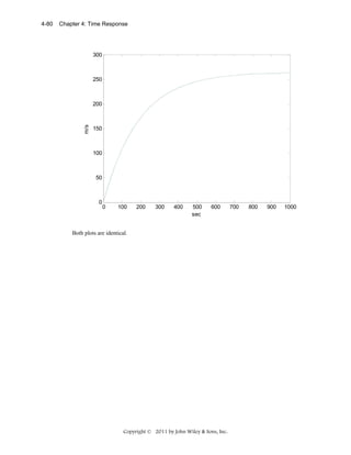
![5-2 Chapter 5: Reduction of Multiple Subsystems
.
x 1 = x2
.
x 2 = - 1.32x2 + 0.8x3
.
10
x 3 = -150x3 +150K( (q i − 0.2x1 )) = -95.49Kx1 - 150x3 + 477.46Kθi
π
θo = 0.2x1
In vector-matrix notation,
.
x =
θo =
c.
T1 =
GL1 =
0
0
-95.49K
0.2
0
1
-1.32
0
0
0
0.8
-150
x +
0
0
477.46K
θ
i
x
76.39
⎛ 10 ⎞
⎛1
⎛1 ⎛ 1
(K)(150) ⎞ (0.8) ⎞ ⎞ (0.2) =
3
⎝π⎠
⎝ s⎠
⎝ s⎠ ⎝ s ⎠
s
−150
−1.32
⎛1
⎛1 ⎛1
⎛ −10 ⎞ −76.39K
=
; GL 2 =
; GL 3 = (K)(150) ⎞ (0.8) ⎞ ⎞ (0.2)
3
⎝ s⎠
⎝ s ⎠ ⎝ s⎠
⎝ π ⎠
s
s
s
Nontouching loops:
198
GL1GL2 = 2
s
Δ = 1 - [GL1 + GL2 + GL3] + [GL1GL2] = 1 +
150
1.32
76.39K
198
+ 2
s + s +
s3
s
Δ1 = 1
T(s) =
T1Δ1
76.39K
= 3
Δ
s +151.32s2 +198s+76.39K
10
π
0.16K
d. The equivalent forward path transfer function is G(s) = s(s+1.32) .
Therefore,
2.55
T(s) = 2
s +1.32s+2.55
The poles are located at -0.66 ± j1.454. ωn = 2.55 = 1.597 rad/s; 2ζωn = 1.32, therefore, ζ = 0.413.
Copyright © 2011 by John Wiley & Sons, Inc.](https://image.slidesharecdn.com/solutionscontrolsystemsengineeringbynormannice6ed-130502172814-phpapp02-131105052456-phpapp01/85/Solutions-control-system-sengineering-by-normannice-6ed-130502172814-phpapp02-189-320.jpg)
![5-4 Chapter 5: Reduction of Multiple Subsystems
b. Using the signal flow graph to write the state equations:
&
x1
&
x2
&
x3
&
x4
= x2
= −1.483 x2 + x3 − 0.125 x4
= −0.24897 x2 − (0.125*0.437) x4
= 2 x1 + 2 x2 − 2 x4 − 2u
In vector-matrix form:
1
⎡0
⎢ 0 −1.483
&
x = ⎢
⎢ 0 −0.24897
⎢
2
⎣2
y = [1 0 0 0]x
0
0
⎤
⎡0⎤
⎢ ⎥
0
−0.125 ⎥
⎥x+⎢ 0 ⎥
⎢0⎥
0 −0.054625⎥
⎥
⎢ ⎥
0
−2
⎦
⎣ −2 ⎦
c.
Program:
numg1=-0.25*[1 0.437];
deng1=poly([-2 -1.29 -0.193 0]);
'G(s)'
G=tf(numg1,deng1)
numh1=[-1 0];
denh1=[0 1];
'H(s)'
H=tf(numh1,denh1)
'Ge(s)'
Ge=feedback(G,H)
'T(s)'
T=feedback(-1*Ge,1)
[numt,dent]=tfdata(T,'V');
[Acc,Bcc,Ccc,Dcc]=tf2ss(numt,dent)
Computer response:
ans =
G(s)
Transfer function:
-0.25 s - 0.1093
-------------------------------------s^4 + 3.483 s^3 + 3.215 s^2 + 0.4979 s
ans =
H(s)
Transfer function:
-s
ans =
Ge(s)
Copyright © 2011 by John Wiley & Sons, Inc.](https://image.slidesharecdn.com/solutionscontrolsystemsengineeringbynormannice6ed-130502172814-phpapp02-131105052456-phpapp01/85/Solutions-control-system-sengineering-by-normannice-6ed-130502172814-phpapp02-191-320.jpg)
![5-6 Chapter 5: Reduction of Multiple Subsystems
11. The Jordan canonical form and the parallel form result from a partial fraction expansion.
12. Parallel form
13. The system poles, or eigenvalues
14. The system poles including all repetitions of the repeated roots
15. Solution of the state variables are achieved through decoupled equations. i.e. the equations are solvable
individually and not simultaneously.
16. State variables can be identified with physical parameters; ease of solution of some representations
17. Systems with zeros
18. State-vector transformations are the transformation of the state vector from one basis system to another.
i.e. the same vector represented in another basis.
19. A vector which under a matrix transformation is collinear with the original. In other words, the length
of the vector has changed, but not its angle.
20. An eigenvalue is that multiple of the original vector that is the transformed vector.
21. Resulting system matrix is diagonal.
SOLUTIONS TO PROBLEMS
1.
a. Combine the inner feedback and the parallel pair.
Multiply the blocks in the forward path and apply the feedback formula to get,
50(s-2)
.
T(s) = 3 2
s +s +150s-100
b.
Program:
'G1(s)'
G1=tf(1,[1 0 0])
'G2(s)'
G2=tf(50,[1 1])
'G3(s)'
G3=tf(2,[1 0])
'G4(s)'
G4=tf([1 0],1)
'G5(s)'
G5=2
'Ge1(s)=G2(s)/(1+G2(s)G3(s))'
Ge1=G2/(1+G2*G3)
'Ge2(s)=G4(s)-G5(s)'
Copyright © 2011 by John Wiley & Sons, Inc.](https://image.slidesharecdn.com/solutionscontrolsystemsengineeringbynormannice6ed-130502172814-phpapp02-131105052456-phpapp01/85/Solutions-control-system-sengineering-by-normannice-6ed-130502172814-phpapp02-193-320.jpg)
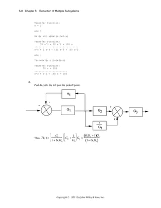
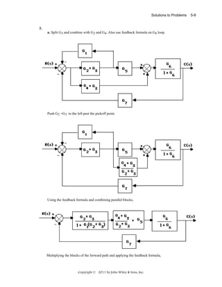
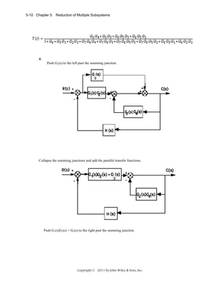
![Solutions to Problems
Collapse summing junctions and add feedback paths.
Applying the feedback formula,
T (s) =
=
G3 ( s) + G1 ( s)G2 ( s)
⎡
⎤
G2 ( s )G4 ( s)
1 + [G3 ( s ) + G1 ( s )G2 ( s)] ⎢ H +
G3 ( s ) + G1 ( s )G2 ( s ) ⎥
⎣
⎦
G3 ( s ) + G1 ( s )G2 ( s )
1 + H [G3 ( s ) + G1 ( s )G2 ( s )] + G2 ( s )G4 ( s )
Copyright © 2011 by John Wiley & Sons, Inc.
5-11](https://image.slidesharecdn.com/solutionscontrolsystemsengineeringbynormannice6ed-130502172814-phpapp02-131105052456-phpapp01/85/Solutions-control-system-sengineering-by-normannice-6ed-130502172814-phpapp02-198-320.jpg)
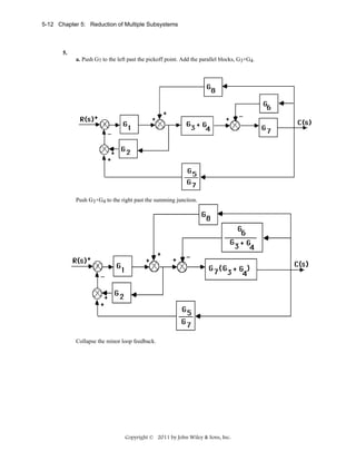
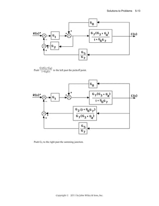
![5-14 Chapter 5: Reduction of Multiple Subsystems
Add the parallel feedback paths to get the single negative feedback,
G2(1+G6G7) G8
G5
H(s) = G + G (G +G ) - G . Thus,
7
7 3 4
1
T(s) =
b.
Program:
G1=tf([0 1],[1 7]);
%G1=1/s+7 input transducer
G2=tf([0 0 1],[1 2 3]);
%G2=1/s^2+2s+3
G3=tf([0 1],[1 4]);
%G3=1/s+4
G4=tf([0 1],[1 0]);
%G4=1/s
G5=tf([0 5],[1 7]);
%G5=5/s+7
G6=tf([0 0 1],[1 5 10]);
%G6=1/s^2+5s+10
G7=tf([0 3],[1 2]);
%G7=3/s+2
G8=tf([0 1],[1 6]);
%G8=1/s+6
G9=tf([1],[1]);
%Add G9=1 transducer at the input
T1=append(G1,G2,G3,G4,G5,G6,G7,G8,G9);
Q=[1 -2 -5 9
2 1 8 0
3 1 8 0
4 1 8 0
5 3 4 -6
6 7 0 0
7 3 4 -6
8 7 0 0];
inputs=9;
outputs=7;
Ts=connect(T1,Q,inputs,outputs);
T=tf(Ts)
Copyright © 2011 by John Wiley & Sons, Inc.](https://image.slidesharecdn.com/solutionscontrolsystemsengineeringbynormannice6ed-130502172814-phpapp02-131105052456-phpapp01/85/Solutions-control-system-sengineering-by-normannice-6ed-130502172814-phpapp02-201-320.jpg)
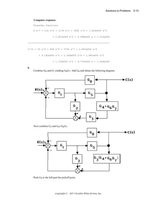
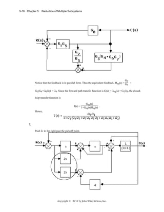
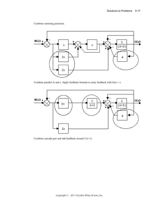
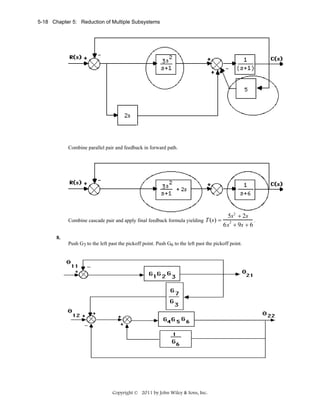
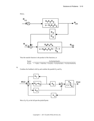
![5-24 Chapter 5: Reduction of Multiple Subsystems
16.
The equivalent forward-path transfer function is
G(s) =
10K1
. Hence,
s[s + (10K2 + 2)]
G(s)
10K1
= 2
. Since
1 + G(s) s + (10K2 + 2)s + 10K1
4
π
Ts =
= 3.2, ∴ Re = 1.25; and Tp =
= 1.5, ∴ Im=2.09 . The poles are thus at
Re
Im
T (s) =
–1.25+j2.09. Hence,
ωn = 1.252 + 2.092 = 10 K1
. Thus, K1 = 0.593. Also, (10K2 + 2)/2 = Re
= 1.25. Hence, K2 = 0.05.
17.
a. For the inner loop, Ge(s) =
Ge(s)
20
, and He(s) = 0.2s. Therefore, Te(s) = 1 + G (s)H (s) =
e
e
s(s + 12)
20
s(s+16) . Combining with the equivalent transfer function of the parallel pair, Gp(s) = 20, the system
400
is reduced to an equivalent unity feedback system with G(s) = Gp(s) Te(s) = s(s+16) . Hence, T(s) =
400
G(s)
1+G(s) = s2+16s+400 .
b. ωn2 = 400; 2ζωn = 16. Therefore, ωn = 20, and ζ = 0.4.
Ts =
4
=0.5; Tp =
ζωn
ω
π
2
n 1-ζ
%OS = e −ζπ /
1−ζ
2
x100 = 25.38 ;
=0.171. From Figure 4.16, ωnTr = 1.463. Hence, Tr = 0.0732.
ωd = Im = ωn 1 - ζ2 = 18.33.
18.
38343
; from which, 2ζωn = 200 and ωn = 38343 = 195.81. Hence,
s + 200s + 38343
2
π
ζ = 0.511. %OS=e-ζπ / 1-ζ x100 = 15.44% ; Tp =
= 0.0187 s.
ωn 1 − ζ 2
4
= 0.04 s.
Also, Ts =
T ( s) =
2
ζω n
19.
Ei(s)
Eg(s)
2
For the generator, Eg(s) = KfIf(s). But, If(s) = R +L s . Therefore, E (s) = s+1 . For the motor,
f f
i
1
1
1
consider Ra = 2 Ω, the sum of both resistors. Also, Je = Ja+JL(2 )2 = 0.75+4x4 = 1.75; De = DL(2 )2
= 1. Therefore,
Copyright © 2011 by John Wiley & Sons, Inc.](https://image.slidesharecdn.com/solutionscontrolsystemsengineeringbynormannice6ed-130502172814-phpapp02-131105052456-phpapp01/85/Solutions-control-system-sengineering-by-normannice-6ed-130502172814-phpapp02-211-320.jpg)
![5-32 Chapter 5: Reduction of Multiple Subsystems
•
x1 = x 2
•
x2 = x 3
•
x3 = x 4
•
x4 = −80x 2 − 66x3 − 15x 4 + 20r
y = x1
r
1
s
20
1
s
x4
x
3
1
s
1
s
x
2
x
1 1
y
-15
-66
-80
b. G(s) = (
r
20
20
1
1
1
)(
)(
)(
). Hence,
s s + 2 s + 5 s +8
1
s
x
4
1
1
s
x
3
1
-2
From which,
1
s
x
2
-5
1
1
s
x
1
-8
•
x1 = −8x1 + x 2
•
x2 = −5x2 + x 3
•
x3 = −2x3 + x 4
•
x4 = 20r
y = x1
26.
Δ = 1 + [G2G3G4 + G3G4 + G4 + 1] + [G3G4 + G4]; T1 = G1G2G3G4; Δ1 = 1. Therefore,
T(s) =
T1Δ1
G1G2G3G4
= 2 + G G G + 2G G + 2G
Δ
2 3 4
3 4
4
Copyright © 2011 by John Wiley & Sons, Inc.
1
y](https://image.slidesharecdn.com/solutionscontrolsystemsengineeringbynormannice6ed-130502172814-phpapp02-131105052456-phpapp01/85/Solutions-control-system-sengineering-by-normannice-6ed-130502172814-phpapp02-219-320.jpg)
![Solutions to Problems
5-33
27.
Closed-loop gains: G2G4G6G7H3; G2G5G6G7H3; G3G4G6G7H3; G3G5G6G7H3; G6H1; G7H2
Forward-path gains: T1 = G1G2G4G6G7; T2 = G1G2G5G6G7; T3 = G1G3G4G6G7; T4 =
G1G3G5G6G7
Nontouching loops 2 at a time: G6H1G7H2
Δ = 1 - [H3G6G7(G2G4 + G2G5 + G3G4 + G3G5) + G6H1 + G7H2] + [G6H1G7H2]
Δ1 = Δ2 = Δ3 = Δ4 = 1
T(s) =
T1Δ1 + T2Δ2 + T3Δ3 + T4Δ4
Δ
G1G2G4G6G7 + G1G2G5G6G7 + G1G3G4G6G7 + G1G3G5G6G7
= 1 - H G G (G G + G G + G G + G G ) - G H - G H + G H G H
3 6 7 2 4
2 5
3 4
3 5
6 1
7 2
6 1 7 2
28.
1
1
Closed-loop gains: -s2; - s ; - s ; -s2
1
Forward-path gains: T1 = s; T2 = 2
s
Nontouching loops: None
1 1
Δ = 1 - (-s2 - s - s - s2)
Δ1 = Δ2 = 1
T1Δ1 + T2Δ2
=
G(s) =
Δ
1
s+ 2
s
s3+1
= 4 2
1 1
2s +s +2s
1 + (s2 + s + s + s2)
29.
G2G3G4G5
G1⎛(1-G H )(1-G H )⎞
2 1
4 2⎠
⎝
T(s) =
=
G2G3G4G5G6G7G8
1 - (1-G H )(1-G H )(1-G H )
2 1
4 2
7 4
G1G2G3G4G5(1-G7H4)
1-G2H1-G4H2+G2G4H1H2-G7H4+G2G7H1H4+G4G7H2H4-G2G4G7H1H2H4-G2G3G4G5G6G7G8
30.
a.
G(s) =
(s + 1)(s + 2)
2
5
6
=
+
2
2 −
(s + 3) (s + 4) (s + 3)
s+3 s+4
Copyright © 2011 by John Wiley & Sons, Inc.](https://image.slidesharecdn.com/solutionscontrolsystemsengineeringbynormannice6ed-130502172814-phpapp02-131105052456-phpapp01/85/Solutions-control-system-sengineering-by-normannice-6ed-130502172814-phpapp02-220-320.jpg)
![5-34 Chapter 5: Reduction of Multiple Subsystems
Writing the state and output equations,
.
x 1 = -3x1 + x2
.
x 2 = -3x2 + r
.
x 3 = -4x3 + r
y = 2x1 - 5x2 + 6x3
In vector-matrix form,
0⎤
⎡−3 1
⎡ 0⎤
x = ⎢ 0 −3 0 ⎥ x + ⎢ 1⎥ r
⎢0
⎢ 1⎥
0 −4 ⎥
⎣
⎦
⎣ ⎦
•
y = [2 −5 6]
b. G(s) =
G(s) =
(s + 2)
3/ 4
1
5/4
1
−
2
2 =−
2 +
2 −
(s + 5) (s + 7)
(s + 5)
s + 5 (s + 7) s + 7
1
s
r
1
x
1
s
1
2
x
1
- 3
4
-5
-5
y
1
1
1
s
x
4
1
s
1
-7
-7
-1
Writing the state and output equations,
.
x 1 = -5x1 + x2
Copyright © 2011 by John Wiley & Sons, Inc.
x
3
- 5
4](https://image.slidesharecdn.com/solutionscontrolsystemsengineeringbynormannice6ed-130502172814-phpapp02-131105052456-phpapp01/85/Solutions-control-system-sengineering-by-normannice-6ed-130502172814-phpapp02-221-320.jpg)
![Solutions to Problems
b.
Writing the state equations,
•
x1 = x 2
•
x2 = x 3
•
x3 = − x1 − 2x2 − 5x3 + r
y = 6x1 + 2x 2 + x3
In vector matrix form,
1
⎡0
x = ⎢0
0
⎢−1 −2
⎣
•
0⎤
⎡ 0⎤
1 ⎥ X + ⎢ 0⎥ r
⎢ 1⎥
−5⎥
⎦
⎣ ⎦
y = [6 2 1]x
Copyright © 2011 by John Wiley & Sons, Inc.
5-37](https://image.slidesharecdn.com/solutionscontrolsystemsengineeringbynormannice6ed-130502172814-phpapp02-131105052456-phpapp01/85/Solutions-control-system-sengineering-by-normannice-6ed-130502172814-phpapp02-224-320.jpg)
![Solutions to Problems
.
x 2 = x1
.
x 1 = - 7x2 - 2x1 + r
y = 3x2 + x1
Putting the equations in order,
.
x 1 = - 2x1 - 7x2 + r
.
x 2 = x1
y = x1 + 3x2
In vector-matrix form,
•
⎡−2 −7⎤
⎡1 ⎤
x=⎢
x + ⎢ ⎥r
⎣1 0⎥
⎦
⎣0 ⎦
y = [1 3]x
Observer canonical form:
s+3
1
G(s) = 2
. Divide each term by 2
s
s +2s+7
G( s) =
and get
3
1
+
s
2
s
1 +
2
7
+
s
2
s
=
C( s)
R( s)
Cross multiplying,
1 3
2
7
( s + 2 ) R(s) = (1 + s + 2 ) C(s)
s
s
Thus,
1
1
s (R(s) - 2C(s)) + s2 (3R(s) - 7C(s)) = C(s)
Drawing the signal-flow graph,
Copyright © 2011 by John Wiley & Sons, Inc.
5-39](https://image.slidesharecdn.com/solutionscontrolsystemsengineeringbynormannice6ed-130502172814-phpapp02-131105052456-phpapp01/85/Solutions-control-system-sengineering-by-normannice-6ed-130502172814-phpapp02-226-320.jpg)
![5-40 Chapter 5: Reduction of Multiple Subsystems
R(s)
1
3
-2
-7
Writing the state and output equations,
.
x 1 = - 2x1 + x2 + r
.
x 2 = - 7x1 + 3r
y = x1
In vector matrix form,
•
⎡−2 1 ⎤
⎡1⎤
x=⎢
⎥ x + ⎢ 3⎥ r
⎣ −7 0 ⎦
⎣ ⎦
y = [1 0]x
b. Controller canonical form:
From the phase-variable form in Problem 5.31(b), reverse the order of the state variables and obtain,
•
x3 = x2
•
x2 = x1
•
x1 = −x 3 − 2x2 − 5x1
y = 6x3 + 2x 2 + x1
Putting the equations in order,
•
x1 = −5x1 − 2x 2 − x3
•
x2 = x1
•
x3 = x2
y = x1 + 2x 2 + 6x3
In vector-matrix form,
Copyright © 2011 by John Wiley & Sons, Inc.](https://image.slidesharecdn.com/solutionscontrolsystemsengineeringbynormannice6ed-130502172814-phpapp02-131105052456-phpapp01/85/Solutions-control-system-sengineering-by-normannice-6ed-130502172814-phpapp02-227-320.jpg)
![Solutions to Problems
5-41
⎡−5 −2 −1⎤
⎡1 ⎤
x = ⎢1
0
0 ⎥ x + ⎢0 ⎥ r
⎢0
⎢0 ⎥
1
0⎥
⎣
⎦
⎣ ⎦
•
y = [1 2 6]x
Observer canonical form:
G(s) =
s2 + 2s + 6
1
. Divide each term by 3 and get
3
2
s + 5s + 2s + 1
s
1 2 6
+ +
s s 2 s3 = C(s)
G(s) =
5 2 1
1 + + 2 + 3 R(s)
s s
s
Cross-multiplying,
⎛1 2 6 ⎞
⎛ 5 2 1
+ 2 + 3 R(s) = 1 + + 2 + 3 ⎞ C(s)
⎝s s
⎝
s s
s ⎠
s ⎠
Thus,
1
1
1
(R(s) − 5c(s)) + 2 (2R(s) − 2C(s)) + 3 (6R(s) − C(s)) = C(s)
s
s
s
Drawing the signal-flow graph,
1
2
6
R(s)
1
s
X3(s)
1
s
1
X2(s)
1
s
1
X1(s)
1
C(s)
-5
-2
-1
Writing the state and output equations,
•
x1 = −5x1 + x 2 + r
•
x2 = −2x1 + x3 + 2r
•
x3 = − x1 + 6r
y = [1 0 0]x
Copyright © 2011 by John Wiley & Sons, Inc.](https://image.slidesharecdn.com/solutionscontrolsystemsengineeringbynormannice6ed-130502172814-phpapp02-131105052456-phpapp01/85/Solutions-control-system-sengineering-by-normannice-6ed-130502172814-phpapp02-228-320.jpg)
![5-42 Chapter 5: Reduction of Multiple Subsystems
In vector-matrix form,
⎡ −5 1 0⎤
⎡1 ⎤
x = ⎢−2 0 1⎥ x + ⎢2 ⎥ r
⎢ −1 0 0⎥
⎢6 ⎥
⎣
⎣ ⎦
⎦
•
y = [1 0 0]x
c. Controller canonical form:
From the phase-variable form in Problem 5.31(c), reverse the order of the state variables and obtain,
.
x 4 = x3
.
x 3 = x2
.
x 2 = x1
.
x 1 = - 4x4 - 6x3 - 5x2 - 3x1 + r
y = x4 + 7x3 + 2x2 + x1
Putting the equations in order,
.
x 1 = - 3x1 - 5x2 - 6x3 - 4x4 + r
.
x 2 = x1
.
x 3 = x2
.
x 4 = x3
y = x1 + 2x2 +7x3 + x4
In vector-matrix form,
⎡−3 −5 −6 −4 ⎤
⎡ 1⎤
•
⎢1 0 0 0 ⎥
⎢ 0⎥
x=
X+
r
⎢0 1 0 0 ⎥
⎢ 0⎥
⎢0 0 1 0 ⎥
⎢ 0⎥
⎣
⎣ ⎦
⎦
y = [1 2 7 1]x
Observer canonical form:
s3+2s2+7s+1
1
G(s) = 4 3 2
. Divide each term by 2
s
s +3s +5s +6s+4
1
+
s
G( s ) =
2
s
3
1 +
+
s
7
+
2
s
5
s
2
+
and get
+
3
1
s
6
s
3
+
4
=
4
s
4
Copyright © 2011 by John Wiley & Sons, Inc.
C( s )
R( s )](https://image.slidesharecdn.com/solutionscontrolsystemsengineeringbynormannice6ed-130502172814-phpapp02-131105052456-phpapp01/85/Solutions-control-system-sengineering-by-normannice-6ed-130502172814-phpapp02-229-320.jpg)
![5-44 Chapter 5: Reduction of Multiple Subsystems
33.
a.
1
1
s x3 1
50
r
1
s
-9
-2
x
2
1
s
1
c= y
-5
-8
-7
-2
-1
Writing the state equations,
•
x1 = −2 x1 + x2
•
x2 = −8 x2 + x3
•
x3 = −50 x1 − 9 x3 + 50r
y = x1
In vector-matrix form,
⎡ −2 1 0 ⎤
⎡0⎤
⎢ 0 −8 1 ⎥ x + ⎢ 0 ⎥ r
x=⎢
⎥
⎢ ⎥
⎢ −50 0 −9 ⎥
⎢50 ⎥
⎣
⎦
⎣ ⎦
y = [1 0 0] x
•
b.
1
r
1
s
x3
10
1 x
2
s
-6
-8
-24
-25
-1
Copyright © 2011 by John Wiley & Sons, Inc.
1
s
x1
x1
c= y](https://image.slidesharecdn.com/solutionscontrolsystemsengineeringbynormannice6ed-130502172814-phpapp02-131105052456-phpapp01/85/Solutions-control-system-sengineering-by-normannice-6ed-130502172814-phpapp02-231-320.jpg)
![Solutions to Problems
Writing the state equations,
•
x1 = x2
•
x2 = −24 x1 − 6 x2 + 10 x3
•
x3 = − x1 + r
y = x1
In vector-matrix form,
1 0⎤
⎡ 0
⎡0 ⎤
⎢ −24 −6 10 ⎥ x + ⎢0 ⎥ r
x=⎢
⎥
⎢ ⎥
⎢ −1 0 0 ⎥
⎢1 ⎥
⎣
⎦
⎣ ⎦
y = [1 0 0] x
•
c.
1
1
160
100
1
s
x
2
1
s
1
x1
r
-1
-1
Tach feedback
before integrator
-1
.
x 1 = x2
.
x 2 = -x2 - x2 + 160(r-x1) = -160x1 -2x2 +160r
y = x1
In vector-matrix form,
1⎤
⎡ 0
⎡ 0 ⎤
⎥ x + ⎢ −160 ⎥ r
⎣ −160 −2 ⎦
⎣
⎦
&
x=⎢
y =
1 0 x
Copyright © 2011 by John Wiley & Sons, Inc.
c= y
5-45](https://image.slidesharecdn.com/solutionscontrolsystemsengineeringbynormannice6ed-130502172814-phpapp02-131105052456-phpapp01/85/Solutions-control-system-sengineering-by-normannice-6ed-130502172814-phpapp02-232-320.jpg)
![5-46 Chapter 5: Reduction of Multiple Subsystems
d. Since
1
1
= 2
, we draw the signal-flow as follows:
(s+1)2
s +2s+1
1
1
1
s
10
16
x
r
1
s
2
x1
2
c= y
-2
-1
-1
Writing the state equations,
.
x 1 = x2
.
x 2 = -x1 - 2x2 + 16(r-c) = -x1 - 2x2 + 16(r - (2x1+x2) = -33x1 - 18x2 + 16r
y = 2x1 + x2
In vector-matrix form,
1 ⎤
⎡ 0
⎡0⎤
⎥ x + ⎢16 ⎥ r
⎣ -33 -18⎦
⎣ ⎦
&
x=⎢
&
y = [2 1] x
34.
a. Phase-variable form:
10
T(s) = 3 2
s +3s +2s+10
10
1
s
x3
r= u
1
s
x2
1
s
-3
-2
-10
Writing the state equations,
.
x 1 = x2
.
x 2 = x3
.
x 3 = -10x1 -2x2 -3x3 + 10u
y = x1
In vector-matrix form,
Copyright © 2011 by John Wiley & Sons, Inc.
x1
c= y](https://image.slidesharecdn.com/solutionscontrolsystemsengineeringbynormannice6ed-130502172814-phpapp02-131105052456-phpapp01/85/Solutions-control-system-sengineering-by-normannice-6ed-130502172814-phpapp02-233-320.jpg)
![Solutions to Problems
x =
0
0
-10
1
0
-2
0
1
-3
0
0
10
x +
u
1 0 0 x
y=
b. Parallel form:
5
-10
5
G(s) = s + s+1 + s+2
1
s
x1
1
5
r=u
-10
1
r=u
1
s
x2
1
c=y
-1
1
s
5
x3
1
-2
-1
Writing the state equations,
.
x 1 = 5(u - x1 - x2 - x3) = -5x1 -5x2 -5x3 +5u
.
x 2 = -10(u - x1 - x2 - x3) - x2 = 10x1 + 9x2 + 10x3 - 10u
.
x 3 = 5(u - x1 - x2 - x3) - 2x3 = -5x1 -5x2 -7x3 +5u
y = x 1 + x 2 + x3
In vector-matrix form,
⎡−5 −5 −5⎤
⎡ 5 ⎤
x = ⎢10 9 10 ⎥ x + ⎢ −10 ⎥u
⎢−5 −5 −7⎥
⎢ 5 ⎥
⎣
⎦
⎣
⎦
•
y = [1 1 1]x
35.
a.
T (s) =
10(s2 + 5s + 6)
s4 + 16s3 + 99s2 + 244s + 180
Copyright © 2011 by John Wiley & Sons, Inc.
5-47](https://image.slidesharecdn.com/solutionscontrolsystemsengineeringbynormannice6ed-130502172814-phpapp02-131105052456-phpapp01/85/Solutions-control-system-sengineering-by-normannice-6ed-130502172814-phpapp02-234-320.jpg)
![5-48 Chapter 5: Reduction of Multiple Subsystems
Drawing the signal-flow diagram,
1
5
1
s
10
r
16
1
s
1
s
1
s
x4
x3
x2
6
y
x1
99
244
180
Writing the state and output equations,
•
x1 = x 2
•
x2 = x 3
•
x3 = x 4
•
x1 = −180x1 − 244x2 − 99x 3 − 16x4 + 10r
y = 6x1 + 5x2 + x 3
In vector-matrix form,
⎡ 0
•
⎢ 0
x=
⎢ 0
⎢− 180
⎣
1
0
0
1
0
0
−244 −99
0 ⎤
⎡0⎤
0 ⎥
⎢0⎥
x+
r
⎢0⎥
1 ⎥
⎢10 ⎥
−16⎥
⎣ ⎦
⎦
y = [6 5 1 0]x
b.
G(s) =
10(s + 2)(s + 3)
1/ 3 10 / 3 15
12
=
−
+
−
(s + 1)(s + 4)(s + 5)(s + 6) s + 1 s + 4 s + 5 s + 6
Drawing the signal-flow diagram and including the unity-feedback path,
Copyright © 2011 by John Wiley & Sons, Inc.](https://image.slidesharecdn.com/solutionscontrolsystemsengineeringbynormannice6ed-130502172814-phpapp02-131105052456-phpapp01/85/Solutions-control-system-sengineering-by-normannice-6ed-130502172814-phpapp02-235-320.jpg)
![Solutions to Problems
1
s
1
3
1
r=u
-1
− 10
3
x1
1
s
-4
15
1
1
y
x2
1
1
s
-5
-12
1
x3
1
1
s
-6
x4
-1
Writing the state and output equations,
•
1
x1 = (u − x1 − x2 − x3 − x 4 ) − x1
3
•
−10
x2 =
(u − x1 − x 2 − x3 − x4 ) − 4x2
3
•
x3 = 15(u − x1 − x2 − x3 − x 4 ) − 5x 3
•
x4 = −12(u − x1 − x 2 − x3 − x4 ) − 12x4
y = x1 + x2 + x 3 + x 4
In vector-matrix form,
⎡− 4 − 1 − 1 − 1 ⎤
⎡ 1 ⎤
3
3
3⎥
⎢ 3
⎢ 3 ⎥
•
2 10
10
10
10
⎥ x + ⎢− ⎥u
−
x=⎢
3
3
3
3
3
⎢−15 −15 −20 −15⎥
⎢ 15 ⎥
⎥
⎥
⎢
⎢
12 12
0 ⎦
⎣ 12
⎣ −12 ⎦
y = [1 1 1 1]x
36.
Program:
'(a)'
'G(s)'
G=zpk([-2 -3],[-1 -4 -5 -6],10)
Copyright © 2011 by John Wiley & Sons, Inc.
5-49](https://image.slidesharecdn.com/solutionscontrolsystemsengineeringbynormannice6ed-130502172814-phpapp02-131105052456-phpapp01/85/Solutions-control-system-sengineering-by-normannice-6ed-130502172814-phpapp02-236-320.jpg)
![5-50 Chapter 5: Reduction of Multiple Subsystems
'T(s)'
T=feedback(G,1,-1)
[numt,dent]=tfdata(T,'v');
'Find controller canonical form'
[Acc,Bcc,Ccc,Dcc]=tf2ss(numt,dent)
A1=flipud(Acc);
'Transform to phase-variable form'
Apv=fliplr(A1)
Bpv=flipud(Bcc)
Cpv=fliplr(Ccc)
'(b)'
'G(s)'
G=zpk([-2 -3],[-1 -4 -5 -6],10)
'T(s)'
T=feedback(G,1,-1)
[numt,dent]=tfdata(T,'v');
'Find controller canonical form'
[Acc,Bcc,Ccc,Dcc]=tf2ss(numt,dent)
'Transform to modal form'
[A,B,C,D]=canon(Acc,Bcc,Ccc,Dcc,'modal')
Computer response:
ans =
(a)
ans =
G(s)
Zero/pole/gain:
10 (s+2) (s+3)
----------------------(s+1) (s+4) (s+5) (s+6)
ans =
T(s)
Zero/pole/gain:
10 (s+2) (s+3)
-----------------------------------------(s+1.264) (s+3.412) (s^2 + 11.32s + 41.73)
ans =
Find controller canonical form
Acc =
-16.0000
1.0000
0
0
Bcc =
-99.0000 -244.0000 -180.0000
0
0
0
1.0000
0
0
0
1.0000
0
1
0
0
0
Copyright © 2011 by John Wiley & Sons, Inc.](https://image.slidesharecdn.com/solutionscontrolsystemsengineeringbynormannice6ed-130502172814-phpapp02-131105052456-phpapp01/85/Solutions-control-system-sengineering-by-normannice-6ed-130502172814-phpapp02-237-320.jpg)
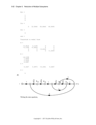
![Solutions to Problems
.
x 1 = x2
.
x 2 = - x1 + x 3
.
x 3 = x4
.
x 4 = x1 - x 2 + r
y = - x 1 + x2
In vector-matrix form,
0
-1
x = 0
1
1
0
0
-1
0
1
0
0
0
0
0 x + 0 r
0
1
1
0
y = c = [-1 1 0 0] x
38.
a.
..
.
.
θ 1 + 5θ 1 + 6θ1 - 3θ 2 - 4θ2 = 0
.
..
.
-3θ 1 - 4θ1 + θ 2 + 5θ 2 + 5θ2 = T
or
..
.
.
θ 1 = - 5θ 1 - 6θ1 + 3θ 2 + 4θ2
..
.
.
θ 2 = 3θ 1 + 4θ1 - 5θ 2 - 5θ2 + T
.
.
Letting, θ1 = x1 ; θ 1 = x2 ; θ2 = x3 ; θ 2 = x4 ,
1
s
4
3
1
x2 s
x1
-5
-6
4
3
1
s
T
1
x4 s
1
-5
-5
Copyright © 2011 by John Wiley & Sons, Inc.
x3
5-53](https://image.slidesharecdn.com/solutionscontrolsystemsengineeringbynormannice6ed-130502172814-phpapp02-131105052456-phpapp01/85/Solutions-control-system-sengineering-by-normannice-6ed-130502172814-phpapp02-240-320.jpg)
![5-54 Chapter 5: Reduction of Multiple Subsystems
where x = θ.
b. Using the signal-flow diagram,
.
x 1 = x2
.
x 2 = -6x1 - 5x2 + 4x3 + 3x4
.
x 3 = x4
.
x 4 = 4x1 + 3x2 - 5x3 - 5x4 + T
y = x3
In vector-matrix form,
0 1 0 0
0
-6 -5 4 3
0
.
x=
x+
T
0 0 0 1
0
4 3 -5 -5
1
y= 0 0 1 0 x
39.
Program:
numg=7;
deng=poly([0 -9 -12]);
G=tf(numg,deng);
T=feedback(G,1)
[numt,dent]=tfdata(T,'v')
[A,B,C,D]=tf2ss(numt,dent);
'(a)'
A=flipud(A);
A=fliplr(A)
B=flipud(B)
C=fliplr(C)
'(b)'
[a,b,c,d]=canon(A,B,C,D)
%Obtain controller canonical form
%Display label
%Convert to phase-variable form
%Convert to phase-variable form
%Convert to phase-variable form
%Convert to phase-variable form
%Display label
%Convert to parallel form
Computer response:
Transfer function:
7
-----------------------s^3 + 21 s^2 + 108 s + 7
numt =
0
0
0
7
21
108
7
dent =
1
Copyright © 2011 by John Wiley & Sons, Inc.](https://image.slidesharecdn.com/solutionscontrolsystemsengineeringbynormannice6ed-130502172814-phpapp02-131105052456-phpapp01/85/Solutions-control-system-sengineering-by-normannice-6ed-130502172814-phpapp02-241-320.jpg)
![Solutions to Problems
5-57
.
x 2 = B2C1x1 + A2x2
y = C1x1
In vector-matrix form,
x1 = A 1 - B1 C2
B 2 C1
A2
x2
x1
y = C1 0
x2
x1 + B 1 r
x2
0
43.
•
z = P −1 APz + P −1 Bu
y = CPz
⎡ −4 9 − 3 ⎤
⎡ -0.2085 -0.3029 -0.1661⎤
⎢ 0 −4 7 ⎥ ; ∴ P = ⎢ 0.0228 -0.1075 -0.0912 ⎥
P =⎢
⎥
⎢
⎥
⎢ − 1 −4 − 9 ⎥
⎢ 0.0130 0.0814 -0.0521⎥
⎣
⎦
⎣
⎦
−1
⎡ 18.5961 25.4756
P AP = ⎢ -12.9023 -28.8893
⎢
⎢ -0.5733 11.4169
⎣
−1
5.6156 ⎤
⎡ −58⎤
⎥ ; P -1B = ⎢ 63 ⎥ ; CP = 1.5668 3.0423 2.7329
-8.3909 ⎥
[
]
⎢
⎥
⎢ −12 ⎥
5.2932 ⎥
⎦
⎣
⎦
44.
•
z = P -1 APz + P -1Bu
y = CPz
⎡5 −4 9 ⎤
P = ⎢6 −7 6 ⎥ ;
⎢
⎥
⎢6 −5 −3⎥
⎣
⎦
⎡ -28.2857
-1
P AP = ⎢ -18.3061
⎢
⎢ 5.3878
⎣
-1
⎡0.3469 -0.3878 0.2653 ⎤
P= ⎢ 0.3673 -0.4694 0.1633 ⎥
⎢
⎥
⎢0.0816 0.0068 -0.0748= ⎥
⎣
⎦
40.8095 -40.9048 ⎤
⎡ 61⎤
⎥ ; P -1B = ⎢82 ⎥ ; CP = -2.0816 2.6599 -1.2585
28.2245 -37.4694 ⎥
[
]
⎢ ⎥
⎢74 ⎥
-6.5510 -5.9388 ⎥
⎦
⎣ ⎦
45.
Eigenvalues are -1, -2, and -3 since,
|λΙ - A | = (λ + 3) (λ + 2) (λ + 1)
Solving for the eigenvectors, Ax = λx
or,
Copyright © 2011 by John Wiley & Sons, Inc.](https://image.slidesharecdn.com/solutionscontrolsystemsengineeringbynormannice6ed-130502172814-phpapp02-131105052456-phpapp01/85/Solutions-control-system-sengineering-by-normannice-6ed-130502172814-phpapp02-244-320.jpg)
![5-58 Chapter 5: Reduction of Multiple Subsystems
x3
x2
For λ = -1, x2 = 0, x1 = x3 . For λ = -2, x1 = x2 = 2 . For λ = -3, x1 = - 2 , x2 = x3 . Thus,
.
z = P-1APz + P-1Bu ; y = CPz, where
46.
Eigenvalues are 1, -2, and 3 since,
|λI - A | = (λ - 3) (λ + 2) (λ - 1)
Solving for the eigenvectors, Ax = λx
or,
x3
For λ = 1, x1 = x2 = 2 . For λ = -2, x1 = 2x3, x2 = -3x3. For λ = 3, x1 = x3 , x2 = -2x3 . Thus,
.
z = P-1APz + P-1Bu ; y = CPz, where
47.
Program:
A=[-10 -3 7;18.25 6.25 -11.75;-7.25 -2.25 5.75];
B=[1;3;2];
C=[1 -2 4];
[P,d]=eig(A);
Ad=inv(P)*A*P
Bd=inv(P)*B
Cd=C*P
Copyright © 2011 by John Wiley & Sons, Inc.](https://image.slidesharecdn.com/solutionscontrolsystemsengineeringbynormannice6ed-130502172814-phpapp02-131105052456-phpapp01/85/Solutions-control-system-sengineering-by-normannice-6ed-130502172814-phpapp02-245-320.jpg)
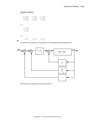
![5-64 Chapter 5: Reduction of Multiple Subsystems
.
x1 = x2
.
x2 = −3x 2 + x 3
.
x3 = x 4
.
x4 = −5Kx1 − 5x 3 − 2x 4 + 5Ku
y = x1
In vector-matrix form:
⎡ 0
.
⎢ 0
x=
⎢ 0
⎢ −5K
⎣
1 0
−3 1
0 0
0 −5
0⎤ ⎡ 0 ⎤
0⎥ ⎢ 0 ⎥
u
x+
1⎥ ⎢ 0 ⎥
−2 ⎥ ⎢ 5K⎥
⎦ ⎣ ⎦
y = [1 0 0 0]x
c.
Program:
for K=1:1:5
numt=5*K;
dent=[1 5 11 15 5*K];
T=tf(numt,dent);
hold on;
subplot(2,3,K);
step(T,0:0.01:20)
title(['K=',int2str(K)])
end
Computer response:
Copyright © 2011 by John Wiley & Sons, Inc.](https://image.slidesharecdn.com/solutionscontrolsystemsengineeringbynormannice6ed-130502172814-phpapp02-131105052456-phpapp01/85/Solutions-control-system-sengineering-by-normannice-6ed-130502172814-phpapp02-251-320.jpg)
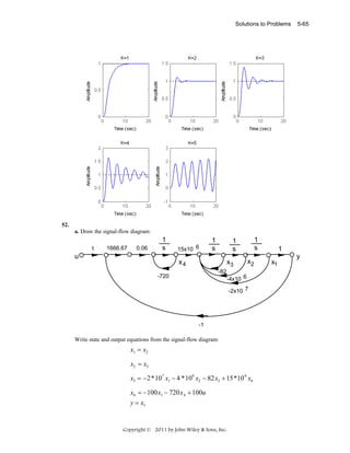
![5-66 Chapter 5: Reduction of Multiple Subsystems
In vector-matrix form:
⎡ 0
.
⎢ 0
x=
⎢ −2*107
⎢ −100
⎣
1
0
−4 *10 6
0
0
0 ⎤
⎡ 0 ⎤
1
0 ⎥
⎢ 0 ⎥
u
x+
6⎥
⎢ 0 ⎥
−82 15*10
⎢100⎥
0
−720 ⎥
⎦
⎣ ⎦
y = [1 0 0 0]x
b.
Program:
numg=1666.67*0.06*15e6;
deng=conv([1 720],[1 82 4e6 2e7]);
'G(s)'
G=tf(numg,deng)
'T(s)'
T=feedback(G,1)
step(T)
Computer response:
ans =
G(s)
Transfer function:
1.5e009
---------------------------------------------------s^4 + 802 s^3 + 4.059e006 s^2 + 2.9e009 s + 1.44e010
ans =
T(s)
Transfer function:
1.5e009
---------------------------------------------------s^4 + 802 s^3 + 4.059e006 s^2 + 2.9e009 s + 1.59e010
Copyright © 2011 by John Wiley & Sons, Inc.](https://image.slidesharecdn.com/solutionscontrolsystemsengineeringbynormannice6ed-130502172814-phpapp02-131105052456-phpapp01/85/Solutions-control-system-sengineering-by-normannice-6ed-130502172814-phpapp02-253-320.jpg)
![Solutions to Problems
53.
-272(s2+1.9s+84)
a. Phase-variable from: G(s) = 3
s +17.1s2+34.58s-123.48
Drawing the signal-flow diagram:
1
1.9
1
s
-272
u
-17.1
1
s
1
s
x3
x2
84
x1
-34.58
123.48
Writing the state and output equations:
.
x1 = x2
.
x2 = x3
.
x3 = 123.48x1 − 34.58x 2 − 17.1x3 − 272u
y = 84x1 + 1.9x2 + x3
In vector-matrix form:
1
0 ⎤
⎡ 0
⎡ 0 ⎤
x=⎢ 0
0
1 ⎥x + ⎢ 0 ⎥u
⎢123.48 −34.58 −17.1⎥
⎢ −272⎥
⎦
⎦
⎣
⎣
.
y = [84 1.9 1]x
-272(s2+1.9s+84)
b. Controller canonical form: G(s) = 3
s +17.1s2+34.58s-123.48
Drawing the signal-flow diagram:
Copyright © 2011 by John Wiley & Sons, Inc.
y
5-67](https://image.slidesharecdn.com/solutionscontrolsystemsengineeringbynormannice6ed-130502172814-phpapp02-131105052456-phpapp01/85/Solutions-control-system-sengineering-by-normannice-6ed-130502172814-phpapp02-254-320.jpg)
![5-68 Chapter 5: Reduction of Multiple Subsystems
1
1.9
1
s
-272
1
s
1
s
84
y
u
-17.1
x1
x2
x3
-34.58
123.48
Writing the state and output equations:
.
.
x1 = −17.1x1 − 34.58x2 + 123.48x3 − 272u
.
x2 = x1
.
x3 = x 2
y = x1 + 1.9x2 + 84x3
In vector-matrix form:
⎡ −17.1 −34.58 123.48⎤
⎡ −272⎤
x=⎢ 1
0
0 ⎥x + ⎢ 0 ⎥u
⎢ 0
⎢ 0 ⎥
1
0 ⎥
⎦
⎦
⎣
⎣
.
y = [1 1.9 84]x
c. Observer canonical form: Divide by highest power of s and obtain
-272 516.8 22848
s - s2 - s3
G(s) =
17.1 34.58 123.48
1+ s + 2 s
s3
Cross multiplying,
-272 516.8 22848
17.1 34.58 123.48
[ s - 2 - 3 ]R(s) = [ 1 + s + 2 ]C(s)
s
s
s
s3
Rearranging,
1
1
1
C(s) = s [ -272R(s) - 17.1C(s)] + 2 [ -516.8R(s) - 34.58C(s)] + 3 [ -22848R(s) + 123.48C(s)]
s
s
Drawing the signal-flow diagram, where r = u and y = c:
Copyright © 2011 by John Wiley & Sons, Inc.](https://image.slidesharecdn.com/solutionscontrolsystemsengineeringbynormannice6ed-130502172814-phpapp02-131105052456-phpapp01/85/Solutions-control-system-sengineering-by-normannice-6ed-130502172814-phpapp02-255-320.jpg)
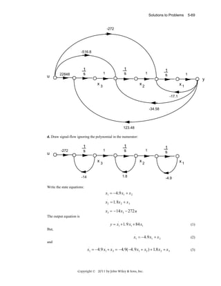
![5-70 Chapter 5: Reduction of Multiple Subsystems
Substituting Eqs. (2) and (3) into (1) yields,
y = 98.7x1 − 1.2x 2 + x 3
In vector-matrix form:
0 ⎤
⎡ −4.9 1
⎡ 0 ⎤
x=⎢ 0
1.8 1 ⎥ x + ⎢ 0 ⎥ u
⎢ 0
⎢ −272 ⎥
0 −14⎥
⎦
⎦
⎣
⎣
.
y = [98.7
−1.2 1]x
e. Expand as partial fractions:
G s
= − 479.38
1 − 232.94 1 + 440.32 1
s + 14
s − 1.8
s + 4.9
Draw signal-flow diagram:
1
s
-14
-479.38
u
-232.94
1
x1
1.8
440.32
1
1
s
1
y
x
2
1
s
-4.9
x
1
3
Write state and output equations:
.
x1 = −14x1 + −479.38u
.
.
x2 = 1.8x 2 − 232.94u
.
x3 = −4.9x3 + 440.32u
y = x1 + x2 + x3
In vector-matrix form:
0 ⎤
⎡ −14 0
⎡ −479.38 ⎤
x = ⎢ 0 1.8
0 ⎥ x + ⎢ −232.94 ⎥u
⎢ 0
⎢ 440.32 ⎥
0 −4.9⎥
⎦
⎦
⎣
⎣
.
y = [1 1 1]x
Copyright © 2011 by John Wiley & Sons, Inc.](https://image.slidesharecdn.com/solutionscontrolsystemsengineeringbynormannice6ed-130502172814-phpapp02-131105052456-phpapp01/85/Solutions-control-system-sengineering-by-normannice-6ed-130502172814-phpapp02-257-320.jpg)
![Solutions to Problems
54.
Push Pitch Gain to the right past the pickoff point.
Collapse the summing junctions and add the feedback transfer functions.
Apply the feedback formula and obtain,
T (s) =
G(s)
0.25(s + 0.435)
= 4
3
1 + G(s) H( s) s + 3.4586s + 3.4569s2 + 0.9693s + 0.15032
55.
Program:
numg1=-0.125*[1 0.435]
deng1=conv([1 1.23],[1 0.226 0.0169])
'G1'
G1=tf(numg1,deng1)
'G2'
G2=tf(2,[1 2])
G3=-1
'H1'
H1=tf([-1 0],1)
'Inner Loop'
Ge=feedback(G1*G2,H1)
'Closed-Loop'
T=feedback(G3*Ge,1)
Computer response:
numg1 =
-0.1250
-0.0544
Copyright © 2011 by John Wiley & Sons, Inc.
5-71](https://image.slidesharecdn.com/solutionscontrolsystemsengineeringbynormannice6ed-130502172814-phpapp02-131105052456-phpapp01/85/Solutions-control-system-sengineering-by-normannice-6ed-130502172814-phpapp02-258-320.jpg)
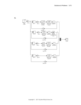
![Solutions to Problems
αβ
Hm
TΔ
(s) = 1 1 =
Hr
Δ
b.
T1 =
α
s
Δ = 1+
Hf
Hr
L1 = −
,
α
s
(s) =
+
β
s
,
1+
α
T1 = α , L1 = −
β
α
+
s
=
β
αβ
s[s + (α + β )]
s
L2 = −
,
s
β
, No non-touching loops.
s
Δ1 = 1
α
T1 Δ 1
=
Δ
c.
α
s2
s
1+
α
s
,
α
s
+
=
β
α
s + (α + β )
s
L2 = −
β
s
, No non-touching loops.
, Δ1 = 1
s
Qi
TΔ
α
αs
(s) = 1 1 =
=
α β s + (α + β )
Hr
Δ
1+ +
s s
Δ = 1+
d.
T1 =
s
αβ
s
Δ = 1+
,
α
s
+
L1 = −
+
β
s
,
Let H r ( s ) =
s
,
L2 = −
β
s
, No non-touching loops.
Δ1 = 1
Qo
TΔ
(s) = 1 1 =
Hr
Δ
e.
α
αβ
s
1+
α
s
+
β
=
αβ
s + (α + β )
s
αβ
αβ
K
H r ( s) =
K=
. From part d) q o (∞) = Lim sQo ( s) = Lim s
s →0
s →0
α +β
s + (α + β )
s
constant
From (a)
⎧
⎫
⎧
⎫
αβ
αβ K
hm (t ) = L- 1 {H m ( s )} = L- 1 ⎨
H r ( s )⎬ = L- 1 ⎨ 2
⎬
⎩ s[s + (α + β )]
⎭
⎩ s [s + (α + β )]⎭
K3
⎧K
⎫
K
− (α + β ) t
= L- 1 ⎨ 21 + 2 +
⎬ = K 1t + K 2 + K 3 e
s
s + (α + β ) ⎭
⎩s
Copyright © 2011 by John Wiley & Sons, Inc.
5-75](https://image.slidesharecdn.com/solutionscontrolsystemsengineeringbynormannice6ed-130502172814-phpapp02-131105052456-phpapp01/85/Solutions-control-system-sengineering-by-normannice-6ed-130502172814-phpapp02-262-320.jpg)

![5-78 Chapter 5: Reduction of Multiple Subsystems
c. From the block diagram we get
vo
g m ( Rs || ro )
Ri
=
vi 1 + g m ( Rs || ro ) Ri + Rs
63.
a. Using Mason’s rule
T1 =
Kt
ω2
ω2
εm r
1
ε
= 2 0 2 ; Loops L1 = + 2 0 2
mr and L2 = −
, no non2
2
s +ε
s + ω 0 M US s + ω 0
s + ω0 s + ε
touching loops.
Δ1 = 1
ω 02
ω 02
X 3 T1 Δ 1
s 2 + ω 02
s 2 + ω 02
=
=
=
R
Δ
ω 02
ε mr s 2
ε
ε
1 + mr
− 2
mr 1 +
s + ε s + ω 02 s + ε
( s + ε )( s 2 + ω 02 )
a. From part (a)
ω 02
ε
2
2
s + ω0 s + ε
X1 X 3 ε
=
=
R
R s+ε
ε mr s 2
1+
( s + ε )( s 2 + ω 02 )
64.
a.
>> A=[-100.2 -20.7 -30.7 200.3; 40 -20.22 49.95 526.1;...
0 10.22 -59.95 -526.1; 0 0 0 0];
>> B=[208; -208; -108.8; -1];
>> C = [0 1570 1570 59400];
>> D = -6240;
>> [n,d]=ss2tf(A,B,C,D)
Copyright © 2011 by John Wiley & Sons, Inc.](https://image.slidesharecdn.com/solutionscontrolsystemsengineeringbynormannice6ed-130502172814-phpapp02-131105052456-phpapp01/85/Solutions-control-system-sengineering-by-normannice-6ed-130502172814-phpapp02-265-320.jpg)

![5-80 Chapter 5: Reduction of Multiple Subsystems
>> roots(n)
ans =
1.0e+002 *
-1.34317654991673
-0.78476212102923
-0.54257777928519
-0.02545278053809
>> roots(d)
ans =
0
-92.38329312886714
-66.38046756013043
-21.60623931100260
Note that s
Y
(0) = 68555.14 , follows that
U
6348.17( s + 2.5)(s + 54.3)(s + 78.5)(s + 134.3)
Y
( s) = −
U
s( s + 21.6)(s + 66.4)(s + 92.4)
b.
>> [r,p,k]=residue(n,d)
Copyright © 2011 by John Wiley & Sons, Inc.](https://image.slidesharecdn.com/solutionscontrolsystemsengineeringbynormannice6ed-130502172814-phpapp02-131105052456-phpapp01/85/Solutions-control-system-sengineering-by-normannice-6ed-130502172814-phpapp02-267-320.jpg)
![5-82 Chapter 5: Reduction of Multiple Subsystems
c.
d. The corresponding state space representation is:
&
0
0
0 ⎤ ⎡ x1 ⎤ ⎡ − 73309.5 ⎤
⎡ x1 ⎤ ⎡0
⎢ x ⎥ ⎢0 − 21.6
&
0
0 ⎥ ⎢ x 2 ⎥ ⎢ − 51344.6 ⎥
⎢ 2⎥ = ⎢
⎥u (t )
⎥⎢ ⎥ + ⎢
⎢ x3 ⎥ ⎢0
&
0
0 ⎥ ⎢ x3 ⎥ ⎢ − 363566.8⎥
− 66.4
⎢ ⎥ ⎢
⎥
⎥⎢ ⎥ ⎢
&
0
0
− 9.4⎦ ⎣ x 4 ⎦ ⎣− 68555.14⎦
⎣ x 4 ⎦ ⎣0
⎡ x1 ⎤
⎢x ⎥
y = [1 1 1 1]⎢ 2 ⎥ − 6240 u (t )
⎢ x3 ⎥
⎢ ⎥
⎣ x4 ⎦
65.
a.
>> A = [0 1 0; 0 -68.3 -7.2; 0 3.2 -0.7]
Copyright © 2011 by John Wiley & Sons, Inc.](https://image.slidesharecdn.com/solutionscontrolsystemsengineeringbynormannice6ed-130502172814-phpapp02-131105052456-phpapp01/85/Solutions-control-system-sengineering-by-normannice-6ed-130502172814-phpapp02-269-320.jpg)
![Solutions to Problems
A=
0 1.0000
0
0 -68.3000 -7.2000
0 3.2000 -0.7000
>> [V,D]=eig(A)
V=
1.0000 0.0147 -0.1016
0 -0.9988 0.1059
0 0.0475 -0.9892
D=
0
0
0 -67.9574
0
0
0
0 -1.0426
Matrix V is the sought similarity transformation.
Copyright © 2011 by John Wiley & Sons, Inc.
5-83](https://image.slidesharecdn.com/solutionscontrolsystemsengineeringbynormannice6ed-130502172814-phpapp02-131105052456-phpapp01/85/Solutions-control-system-sengineering-by-normannice-6ed-130502172814-phpapp02-270-320.jpg)
![5-84 Chapter 5: Reduction of Multiple Subsystems
b.
>> Ad = inv(V)*A*V
Ad =
0 -0.0000 -0.0000
0 -67.9574 0.0000
0 -0.0000 -1.0426
>> B = [0;425.4;0]
B=
0
425.4000
0
>> Bd = inv(V)*B
Bd =
4.2030
-428.1077
-20.5661
The diagonalized system is:
Copyright © 2011 by John Wiley & Sons, Inc.](https://image.slidesharecdn.com/solutionscontrolsystemsengineeringbynormannice6ed-130502172814-phpapp02-131105052456-phpapp01/85/Solutions-control-system-sengineering-by-normannice-6ed-130502172814-phpapp02-271-320.jpg)
![Solutions to Problems
5-93
Response of the Mould Level to Simultaneous Step Changes in Reference Input, r(t) = 5 u(t), and Casting
—
Speed, vp (t) = 0.97 u(t) at an Initial Level, Hm (0 ) = – 75
72.
a. Following the procedure described in Chapter 3 we define
V
A
ϕ = ( s + ) X 1 ( s ) . In time domain &&1 −
x
&
x1 = x2 . These equations give
&
⎡ x1 ⎤ ⎡ 0 1⎤ ⎡ x1 ⎤ ⎡ 0 ⎤
⎢ x ⎥ = ⎢ g 0⎥ ⎢ x ⎥ + ⎢ aV ⎥δ
⎥ ⎣ 2 ⎦ ⎢ bh ⎥
⎣ &2 ⎦ ⎢ h
⎣
⎦
⎣ ⎦
⎡V
⎤⎡ x ⎤
ϕ=⎢
1⎥ ⎢ 1 ⎥
⎣ a ⎦ ⎣ x2 ⎦
X1
δ
=
aV
bh
1
s2 −
g
h
aV
V
g
&
δ . ϕ = x1 + x1 and we also define
x1 =
bh
a
h
b. The eigenvalues can be obtained directly from the transfer function poles. Thus
Consider
⎡0
⎢g
⎢h
⎣
λ1 =
1⎤ ⎡ x ⎤
⎥⎢ 1 ⎥ =
0⎥ ⎣ x 2 ⎦
⎦
and
λ12 = ±
g
, the first eigenvector is found from the solution of Ax 1 = λ1 x 1 or
h
g ⎡ x1 ⎤
. This results in x 2 =
h ⎢ x2 ⎥
⎣ ⎦
g
x1 . Arbitrarily let x1 = 1 so the first
h
⎡ 1 ⎤
eigenvector is v 1 = ⎢ g ⎥ .
⎢
⎥
⎣ h⎦
⎡0
g
; Ax 2 = λ1 x 2 or ⎢ g
h
⎢h
⎣
1⎤ ⎡ x ⎤
g ⎡ x1 ⎤
⎥⎢ 1 ⎥ = −
resulting in
0⎥ ⎣ x 2 ⎦
h ⎢ x2 ⎥
⎣ ⎦
⎦
⎡ 1 ⎤
g
x2 = −
x1 . Letting arbitrarily x1 = 1 the second eigenvector is v 2 = ⎢ g ⎥ .
h
⎢
⎥
⎣ h⎦
1 ⎤
⎡ 1
⎢ g
g⎥
c. The similarity transformation matrix is P = [v 1 v 2 ] =
−
⎢
⎥
h⎦
⎣ h
Similarly for
g
h
λ2 = −
Copyright © 2011 by John Wiley & Sons, Inc.](https://image.slidesharecdn.com/solutionscontrolsystemsengineeringbynormannice6ed-130502172814-phpapp02-131105052456-phpapp01/85/Solutions-control-system-sengineering-by-normannice-6ed-130502172814-phpapp02-280-320.jpg)
![5-96 Chapter 5: Reduction of Multiple Subsystems
100
100. Thus, after tachometer compensation, T(s) = 2
. Hence, ωn = 10; 2ζωn = 1+K2.
s +(1+K2)s+100
Therefore, K2 = 2ζωn - 1 = 2(0.69)(10) - 1 = 12.8.
77.
At the N2 shaft, with rotation,θ L (s)
(Jeq s 2 + Deq s)θ L (s) + F(s)r = Teq (s)
F(s) = (Ms 2 + f vs)X(s)
Thus,
( Jeq s2 + Deq s)θ L ( s) + ( Ms2 + f vs) X (s)r = Teq ( s)
But, X(s) = rθ L (s) . Hence,
[(J
eq
]
+ Mr 2 )s 2 + (Deq + fv r 2 )s θ L (s) = Teq (s)
where
Jeq = Ja (2) 2 + J = 5
Deq = Da (2)2 + D = 4 + D
r=2
Thus, the total load inertia and load damping is
J L = J eq + Mr2 = 5 + 4M
DL = Deq + fv r2 = 4 + D + (1)(2)2 = 8 + D
Reflecting JL and DL to the motor yields,
Jm =
(5 + 4M)
(8 + D)
; Dm =
4
4
Thus, the motor transfer function is
θ m (s)
Kt
Ra J m
1
Jm
=
Ea (s) s(s + 1 (D + K t Ka )) s(s + 1 (D + 1))
m
m
Jm
Jm
Ra
The gears are (10/20)(1) = 1/2. Thus, the forward-path transfer function is
1
⎛
⎞
⎜
Jm
⎟1
Ge (s) = (500)
⎜ s(s + 1 (D + 1))⎟ 2
m
⎝
⎠
Jm
Finding the closed-loop transfer function yields,
Copyright © 2011 by John Wiley & Sons, Inc.](https://image.slidesharecdn.com/solutionscontrolsystemsengineeringbynormannice6ed-130502172814-phpapp02-131105052456-phpapp01/85/Solutions-control-system-sengineering-by-normannice-6ed-130502172814-phpapp02-283-320.jpg)
![5-100 Chapter 5: Reduction of Multiple Subsystems
0.7883
fdesired
K
=1
v
0.01 up 1000
1
s
1
s
x4
1
s
x
3
1
s
x2
42.45
82300
fout
x1
-23.59
-9785
-81190
-3.493x10⁶
-0.01
Writing the state and output equations
•
x1 = x 2
•
x2 = x 3
•
x3 = x 4
•
x4 = −23.59x 4 − 9785x3 − 81190x2 − 3493000x1 + 0.01f desired − 0.01 fout
But,
fout = 42.45 * 82300 x1 + 0.7883 *82300 x 2
Substituting fout into the state equations yields
•
x4 = −3527936.35x1 − 81838.7709x 2 − 9785x 3 − 23.59x4 + 0.01fdesired
Putting the state and output equations into vector-matrix form.
0
⎡
•
⎢
0
x=
⎢
0
⎢−3.528x10⁶
⎣
1
0
0 ⎤ ⎡ 0 ⎤
0
1
0 ⎥ ⎢ 0 ⎥
+
fdesired
0
0
1 ⎥ ⎢ 0 ⎥
−81840 −9785 −23.59⎥ ⎢ 0.01⎥
⎦ ⎣
⎦
y = fout = [3494000 64880 0 0]x
Copyright © 2011 by John Wiley & Sons, Inc.](https://image.slidesharecdn.com/solutionscontrolsystemsengineeringbynormannice6ed-130502172814-phpapp02-131105052456-phpapp01/85/Solutions-control-system-sengineering-by-normannice-6ed-130502172814-phpapp02-287-320.jpg)
![Solutions to Problems
80.
a. The transfer function obtained in Problem 3.30 is
Y
− 520s − 10.3844
= 3
by inspection we write the phase-variable form
U 1 s + 2.6817s 2 + 0.11s + 0.0126
&
0
1
0
⎡ x1 ⎤ ⎡
⎤ ⎡ x1 ⎤ ⎡0⎤
⎢x ⎥ = ⎢
⎥ ⎢ x ⎥ + ⎢0 ⎥ u
&
0
0
1
⎢ 2⎥ ⎢
⎥⎢ 2 ⎥ ⎢ ⎥ 1
⎢ x3 ⎥ ⎢ − 0.0126 − 0.11 − 2.6817 ⎥ ⎢ x3 ⎥ ⎢1 ⎥
⎣& ⎦ ⎣
⎦⎣ ⎦ ⎣ ⎦
⎡ x1 ⎤
y = [− 10.3844 − 520 0]⎢ x 2 ⎥
⎢ ⎥
⎢ x3 ⎥
⎣ ⎦
b. We renumber the phase-variable form state variables in reverse order
&
0
1
0
⎡ x3 ⎤ ⎡
⎤ ⎡ x 3 ⎤ ⎡0⎤
⎢x ⎥ = ⎢
⎥ ⎢ x ⎥ + ⎢0⎥ u
&
0
0
1
⎢ 2⎥ ⎢
⎥⎢ 2 ⎥ ⎢ ⎥ 1
⎢ x1 ⎥ ⎢ − 0.0126 − 0.11 − 2.6817 ⎥ ⎢ x1 ⎥ ⎢1⎥
& ⎦ ⎣
⎣
⎦⎣ ⎦ ⎣ ⎦
⎡ x3 ⎤
y = [− 10.3844 − 520 0]⎢ x 2 ⎥
⎢ ⎥
⎢ x1 ⎥
⎣ ⎦
And we rearrange in ascending numerical order to obtain the controller canonical form:
&
⎡ x1 ⎤ ⎡ − 2.6817 − 0.11 − 0.0126 ⎤ ⎡ x1 ⎤ ⎡1 ⎤
⎢x ⎥ = ⎢
⎥ ⎢ x ⎥ + ⎢0 ⎥ u
&
1
0
0
⎢ 2⎥ ⎢
⎥⎢ 2 ⎥ ⎢ ⎥ 1
⎢ x3 ⎥ ⎢
⎥ ⎢ x 3 ⎥ ⎢0 ⎥
0
0
1
⎣& ⎦ ⎣
⎦⎣ ⎦ ⎣ ⎦
⎡ x1 ⎤
y = [0 − 520 − 10.3844]⎢ x 2 ⎥
⎢ ⎥
⎢ x3 ⎥
⎣ ⎦
c. To obtain the observer canonical form we rewrite the system’s transfer function as:
Y
=
U1
520 10.3844
−
s2
s3
2.6817 0.11 0.0126
1+
+ 2 +
s
s
s3
−
We cross-multiply to obtain
Copyright © 2011 by John Wiley & Sons, Inc.
5-101](https://image.slidesharecdn.com/solutionscontrolsystemsengineeringbynormannice6ed-130502172814-phpapp02-131105052456-phpapp01/85/Solutions-control-system-sengineering-by-normannice-6ed-130502172814-phpapp02-288-320.jpg)
![5-102 Chapter 5: Reduction of Multiple Subsystems
⎡ 520 10.3844 ⎤
⎡ 2.6817 0.11 0.0126 ⎤
⎢− s 2 − s 3 ⎥U 1 = Y ⎢1 + s + s 2 + s 3 ⎥
⎣
⎦
⎣
⎦
Combining terms with like powers of integration:
1
[− 2.6817 Y ] + 12 [− 520R − 0.11Y ] + 13 [− 10.3844R − 0.0126Y ]
s
s
s
1⎡
1⎛
1
⎞⎤
= ⎢− 2.6817Y + ⎜ [− 520 R − 0.11Y ] + [− 10.3844 R − 0.0126Y ]⎟⎥
s⎣
s⎝
s
⎠⎦
Y=
We draw the signal flow graph:
The following equations follow:
&
x1 = −2.6817 x1 + x 2
&
x2 = −0.11x1 + x3 − 520r
&
x3 = −0.0126 x1 − 10.38r
y = x1
Which lead to observer canonical form:
Copyright © 2011 by John Wiley & Sons, Inc.](https://image.slidesharecdn.com/solutionscontrolsystemsengineeringbynormannice6ed-130502172814-phpapp02-131105052456-phpapp01/85/Solutions-control-system-sengineering-by-normannice-6ed-130502172814-phpapp02-289-320.jpg)
![Solutions to Problems
&
⎡ x1 ⎤ ⎡ − 2.6817 1 0⎤ ⎡ x1 ⎤ ⎡ 1 ⎤
⎡ x1 ⎤
⎢ x ⎥ = ⎢ − 0.11 0 1 ⎥ ⎢ x ⎥ + ⎢ − 520 ⎥u ; y = [1 0 0]⎢ x ⎥
&
⎢ 2⎥ ⎢
⎥⎢ 2 ⎥ ⎢
⎥ 1
⎢ 2⎥
⎢ x3 ⎥ ⎢ − 0.0126 0 0⎥ ⎢ x3 ⎥ ⎢− 10.38⎥
⎢ x3 ⎥
⎣& ⎦ ⎣
⎦⎣ ⎦ ⎣
⎦
⎣ ⎦
d.
>> A=[-0.04167 0 -0.0058; 0.0217 -0.24 0.0058; 0 100 -2.4];
>> B=[5.2;-5.2;0];
>> C=[0 0 1];
>> [V,D]=eig(A);
>> Bd=inv(V)*B
Bd =
1.0e+002 *
-0.9936 + 0.0371i
-0.9936 - 0.0371i
1.9797
>> Cd = C*V
Cd =
0.9963 0.9963 1.0000
Copyright © 2011 by John Wiley & Sons, Inc.
5-103](https://image.slidesharecdn.com/solutionscontrolsystemsengineeringbynormannice6ed-130502172814-phpapp02-131105052456-phpapp01/85/Solutions-control-system-sengineering-by-normannice-6ed-130502172814-phpapp02-290-320.jpg)
![5-104 Chapter 5: Reduction of Multiple Subsystems
>> D
D=
-0.0192 + 0.0658i
0
0
0
0
-0.0192 - 0.0658i
0
0
-2.6433
So a diagonalized version of the system is
&
0
0
⎡ x1 ⎤ ⎡ − 0.0192 + j 0.0658
⎤ ⎡ x1 ⎤ ⎡− 99.36 + j 3.71⎤
⎢x ⎥ = ⎢
⎥ ⎢ x ⎥ + ⎢ − 99.36 − j 3.71⎥u
&
− 0.0192 − j 0.0658
0
0
⎢ 2⎥ ⎢
⎥⎢ 2 ⎥ ⎢
⎥ 1
⎢ x3 ⎥ ⎢
⎥
− 2.6433⎥ ⎢ x3 ⎥ ⎢
0
0
197.97
⎣& ⎦ ⎣
⎦⎣ ⎦ ⎣
⎦
⎡ x1 ⎤
y = [0.9963 0.9963 1]⎢ x 2 ⎥
⎢ ⎥
⎢ x3 ⎥
⎣ ⎦
81.
a. Substituting all values and transfer functions into the respective blocks of the system
(Figure 4), we get:
Copyright © 2011 by John Wiley & Sons, Inc.](https://image.slidesharecdn.com/solutionscontrolsystemsengineeringbynormannice6ed-130502172814-phpapp02-131105052456-phpapp01/85/Solutions-control-system-sengineering-by-normannice-6ed-130502172814-phpapp02-291-320.jpg)
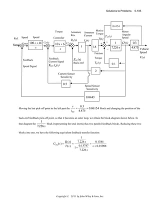
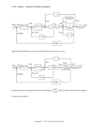
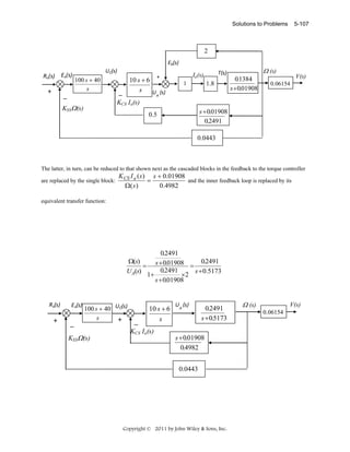
![5-108 Chapter 5: Reduction of Multiple Subsystems
Thus:
Finally
⎛10s + 6⎞ ⎛ 0.2491 ⎞
⎜
⎟⎜
⎟
Ω(s)
0.2491 (10 s + 6)
⎝ s ⎠ ⎝ s + 0.5173
⎠
=
=
UC(s)
⎛10s + 6⎞ ⎛ 0.2491 ⎞ ⎛ s + 0.01908 s (s + 0.5173) + 0.5 (10s + 6) (s+ 0.01908)
⎞
1+⎜
⎟⎜
⎟⎜
⎟
⎝ s ⎠ ⎝ s + 0.5173 ⎝ 0.4982 ⎠
⎠
⎞
0.2491(10 s + 6)
⎛ 100 s + 40 ⎞ ⎛
⎜
⎟⎜
⎜ s ( s + 0.5173) + 0.5 (10 s + 6) (s + 0.01908) ⎟
⎟
s
Ω ( s)
⎝
⎠⎝
⎠
=
Rv ( s )
0.2491 (10 s + 6)
⎛ 100 s + 40 ⎞ ⎛
1 + 0.0443 ⎜
⎟⎜
⎜
s
⎝
⎠ ⎝ s ( s + 0.5173) + 0.5(10 s + 6) (s + 0.01908)
⎞
⎟
⎟
⎠
or
Ω(s)
2491 ( s + 0.4 ) (s + 0.6)
.
=
R (s) s⎛6s2 +3.613s+ 0.0572 +11035⎛ s2 + s + 0.24⎞
⎞ . ⎜
⎟
⎜
⎟
v
⎝
⎠
⎝
⎠
2491 ( s + 0.4 ) ( s + 0.6)
.
=
s
6s3 +14.6442 +11.09 + 2.65
s
Hence:
Ω (s)
15.33 ( s + 0.4 ) ( s + 0.6 )
V ( s)
= 0.06154
=
3
Rv ( s)
Rv ( s)
6 s + 14.644 s 2 + 11.09 s + 2.65
b. Simulink was used to model the HEV cascade control system. That model is shown below. The reference
signal, rv (t), was set as a step input with a zero initial value, a step time = 0 seconds, and a final value
equal to 4 volts [corresponding to the desired final car speed, v (∞ ) = 60 km/h, e.g. a desired final value of
the change in car speed, Δv (∞ ) = 5.55 m/s]. The variables of interest [time, change in car speed,
acceleration, and motor armature current] were output (in array format) to four “workspace” sinks, each of
which was assigned the respective variable name. After the simulation ended, Matlab plot commands were
utilized to obtain and edit the required three graphs. These graphs are shown below.
The simulations show that in response to such a speed reference command, car acceleration would go
initially to a maximum value of 10.22 m/s2 and the motor armature current would reach a maximum value
of 666.7 A. That would require an electric motor drive rated around 80 kW or using both the electric motor
and gas or diesel engine, when fast acceleration is required. Most practical HEV control systems, however,
use current-limiting and acceleration-limiting devices or software programs.
Copyright © 2011 by John Wiley & Sons, Inc.](https://image.slidesharecdn.com/solutionscontrolsystemsengineeringbynormannice6ed-130502172814-phpapp02-131105052456-phpapp01/85/Solutions-control-system-sengineering-by-normannice-6ed-130502172814-phpapp02-295-320.jpg)
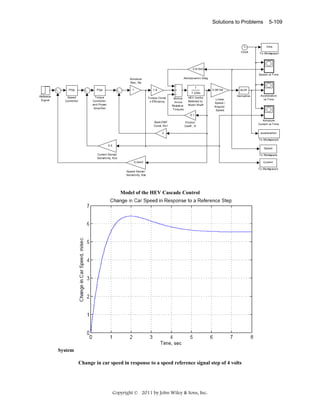
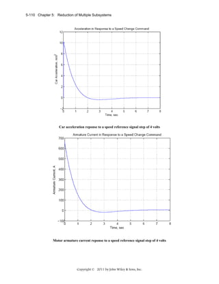


![Solutions to Problems 6-5
5.
s4
1
8
15
s3
4
20
0
s2
3
15
0
s1
6
0
0
s0
15
0
0
ROZ
Even (2): 2 jω; Rest (2): 2 lhp; Total: 2 jω; 2 lhp
6.
s6
1
-6
1
s5
1
0
1
s4
-6
0
-6
s3
-24
0
0
s2
ε
-6
s1
-144/ε
0
s0
-6
-6
ROZ
Even (4): 2 rhp; 2 lhp; Rest (2): 1 rhp; 1 lhp; Total: 3 rhp; 3 lhp
7.
Program:
den=[1 1 -6 0 1 1 -6]
A=roots(den)
Computer response:
den =
1
1
-6
0
1
1
-6
A =
-3.0000
2.0000
-0.7071 + 0.7071i
Copyright © 2011 by John Wiley & Sons, Inc.](https://image.slidesharecdn.com/solutionscontrolsystemsengineeringbynormannice6ed-130502172814-phpapp02-131105052456-phpapp01/85/Solutions-control-system-sengineering-by-normannice-6ed-130502172814-phpapp02-302-320.jpg)
![6-6 Chapter 6: Stability
-0.7071 - 0.7071i
0.7071 + 0.7071i
0.7071 - 0.7071i
8.
Program:
%-det([si() si();sj() sj()])/sj()
%Template for use in each cell.
syms e
%Construct a symbolic object for
%epsilon.
%%%%%%%%%%%%%%%%%%%%%%%%%%$$$$$$$$$%%%%%%%%%%%%%%%%%%%%%%%%%%%%%%%%%
s5=[1 4
3
0
0]
%Create s^5 row of Routh table.
%%%%%%%%%%%%%%%%%%%%%%%%%%%$$$$$$$$$%%%%%%%%%%%%%%%%%%%%%%%%%%%%%%%%
s4=[-1
-4
-2
0
0]
%Create s^4 row of Routh table.
%%%%%%%%%%%%%%%%%%%%%%%%%%%%%%%%%%%%%%%%%%%%%%%%%%%%%%%%%%%%%%%%%%%%
if -det([s5(1) s5(2);s4(1) s4(2)])/s4(1)==0
s3=[e...
-det([s5(1) s5(3);s4(1) s4(3)])/s4(1)
0
0];
%Create s^3 row of Routh table
%if 1st element is 0.
else
s3=[-det([s5(1) s5(2);s4(1) s4(2)])/s4(1) ...
-det([s5(1) s5(3);s4(1) s4(3)])/s4(1)
0
0];
%Create s^3 row of Routh table
%if 1st element is not zero.
end
%%%%%%%%%%%%%%%%%%%%%%%%%%%%%%%%%%%%%%%%%%%%%%%%%%%%%%%%%%%%%%%%%%%%
if -det([s4(1) s4(2);s3(1) s3(2)])/s3(1)==0
s2=[e ...
-det([s4(1) s4(3);s3(1) s3(3)])/s3(1)
0
0];
%Create s^2 row of Routh table
%if 1st element is 0.
else
s2=[-det([s4(1) s4(2);s3(1) s3(2)])/s3(1) ...
-det([s4(1) s4(3);s3(1) s3(3)])/s3(1)
0
0];
%Create s^2 row of Routh table
%if 1st element is not zero.
end
%%%%%%%%%%%%%%%%%%%%%%%%%%%%%%%%%%%%%%%%%%%%%%%%%%%%%%%%%%%%%%%%%%%%
if -det([s3(1) s3(2);s2(1) s2(2)])/s2(1)==0
s1=[e ...
-det([s3(1) s3(3);s2(1) s2(3)])/s2(1)
0
0];
%Create s^1 row of Routh table
%if 1st element is 0.
else
s1=[-det([s3(1) s3(2);s2(1) s2(2)])/s2(1) ...
-det([s3(1) s3(3);s2(1) s2(3)])/s2(1)
0
0];
%Create s^1 row of Routh table
%if 1st element is not zero
end
%%%%%%%%%%%%%%%%%%%%%%%%%%%%%%%%%%%%%%%%%%%%%%%%%%%%%%%%%%%%%%%%%%%%
s0=[-det([s2(1) s2(2);s1(1) s1(2)])/s1(1) ...
-det([s2(1) s2(3);s1(1) s1(3)])/s1(1)
0
0];
%Create s^0 row of Routh table.
%%%%%%%%%%%%%%%%%%%%%%%%%%%%%%%%%%%%%%%%%%%%%%%%%%%%%%%%%%%%%%%%%%%%
's3'
s3=simplify(s3);
pretty(s3)
's2'
%Display label.
%Simplify terms in s^3 row.
%Pretty print s^3 row.
%Display label.
Copyright © 2011 by John Wiley & Sons, Inc.](https://image.slidesharecdn.com/solutionscontrolsystemsengineeringbynormannice6ed-130502172814-phpapp02-131105052456-phpapp01/85/Solutions-control-system-sengineering-by-normannice-6ed-130502172814-phpapp02-303-320.jpg)
![Solutions to Problems 6-7
s2=simplify(s2);
pretty(s2)
's1'
s1=simplify(s1);
pretty(s1)
's0'
s0=simplify(s0);
pretty(s0)
%Simplify terms in s^2 row.
%Pretty print s^2 row.
%Display label.
%Simplify terms in s^1 row.
%Pretty print s^1 row.
%Display label.
%Simplify terms in s^0 row.
%Pretty print s^0 row.
Computer response:
s5 =
1
4
3
0
0
-1
-4
-2
0
0
s4 =
ans =
s3
[e
1
0
0]
-2
0
ans =
s2
[ -1 + 4 e
[- -------[
e
]
0]
]
ans =
s1
[
2
[ 2 e + 1 - 4 e
[- -------------[
-1 + 4 e
0
0
ans =
s0
[-2
0
0
0]
9.
240
T(s) = 4
3 + 35s2 + 50s + 264
s + 10s
Copyright © 2011 by John Wiley & Sons, Inc.
]
]
0]
]](https://image.slidesharecdn.com/solutionscontrolsystemsengineeringbynormannice6ed-130502172814-phpapp02-131105052456-phpapp01/85/Solutions-control-system-sengineering-by-normannice-6ed-130502172814-phpapp02-304-320.jpg)
![6-8 Chapter 6: Stability
2 rhp, 2 lhp
10.
Program:
numg=240;
deng=poly([-1 -2 -3 -4]);
'G(s)'
G=tf(numg,deng)
'Poles of G(s)'
pole(G)
'T(s)'
T=feedback(G,1)
'Poles of T(s)'
pole(T)
Computer response:
ans =
G(s)
Transfer function:
240
--------------------------------s^4 + 10 s^3 + 35 s^2 + 50 s + 24
ans =
Poles of G(s)
ans =
-4.0000
-3.0000
-2.0000
-1.0000
ans =
T(s)
Transfer function:
240
---------------------------------s^4 + 10 s^3 + 35 s^2 + 50 s + 264
ans =
Poles of T(s)
ans =
-5.3948 + 2.6702i
-5.3948 - 2.6702i
0.3948 + 2.6702i
Copyright © 2011 by John Wiley & Sons, Inc.](https://image.slidesharecdn.com/solutionscontrolsystemsengineeringbynormannice6ed-130502172814-phpapp02-131105052456-phpapp01/85/Solutions-control-system-sengineering-by-normannice-6ed-130502172814-phpapp02-305-320.jpg)
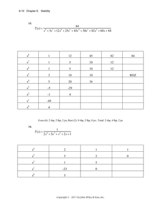
![Solutions to Problems 6-11
Total: 2 lhp, 2 rhp
System is unstable
15.
T (s) =
8
s − 2 s − s + 2s + 4s3 − 8s2 − 4s + 8
7
6
5
4
s7
1
-1
4
-4
s6
-2
2
-8
8
s5
-12
8
-16
0
s4
0.6667
-5.333
8
0
s3
-88
128
0
0
s2
-4.364
8
0
0
s1
-33.33
0
0
0
s0
8
0
0
0
ROZ
Even (6): 3 rhp, 3 lhp; Rest (1): 1 rhp; Total: 4 rhp, 3 lhp
16.
Program:
numg=8;
deng=[1 -2 -1 2 4 -8 -4 0];
'G(s)'
G=tf(numg,deng)
'T(s)'
T=feedback(G,1)
'Poles of T(s)'
pole(T)
Computer response:
ans =
G(s)
Transfer function:
8
----------------------------------------------s^7 - 2 s^6 - s^5 + 2 s^4 + 4 s^3 - 8 s^2 - 4 s
ans =
T(s)
Copyright © 2011 by John Wiley & Sons, Inc.](https://image.slidesharecdn.com/solutionscontrolsystemsengineeringbynormannice6ed-130502172814-phpapp02-131105052456-phpapp01/85/Solutions-control-system-sengineering-by-normannice-6ed-130502172814-phpapp02-308-320.jpg)
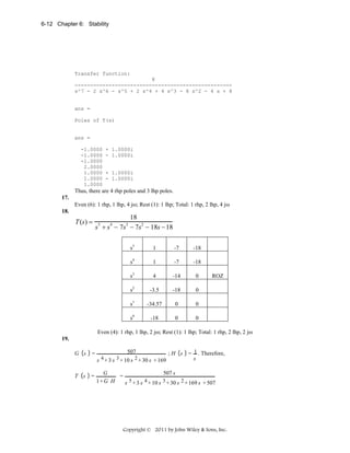
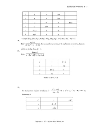
![6-14 Chapter 6: Stability
a)
a < 0, b < 0 ⇒ K > b, K > 0 ⇒ K > 0
b)
a < 0, b > 0 ⇒ K > b, K > 0 ⇒ K > b
c)
a > 0, b < 0 ⇒ K > b, K < 0 ⇒ b < K < 0
d)
a > 0, b > 0 ⇒ K > b, K < 0 ⇒ No solution
23.
T (s ) =
K( s + 3)(s + 5)
(1 + K )s + (8K − 6)s + (8 + 15 K )
2
For 1st column negative
For 1st column positive
s2
1+K
8+15K
K < -1
K > -1
s1
8K-6
0
K < 6/8
K > 6/8
s0
8+15K
0
K < -8/15
K > -8/15
Stable for K > 6/8
24.
Program:
K=[-6:0.00005:0];
for i=1:length(K);
dent=[(1+K(i)) (8*K(i)-6) (8+15*K(i))];
R=roots(dent);
A=real(R);
B=max(A);
if B>0
R
K=K(i)
break
end
end
K=[6:-0.00005:0];
for i=1:length(K);
dent=[(1+K(i)) (8*K(i)-6) (8+15*K(i))];
R=roots(dent);
A=real(R);
B=max(A);
if B>0
R
K=K(i)
break
end
end
Copyright © 2011 by John Wiley & Sons, Inc.](https://image.slidesharecdn.com/solutionscontrolsystemsengineeringbynormannice6ed-130502172814-phpapp02-131105052456-phpapp01/85/Solutions-control-system-sengineering-by-normannice-6ed-130502172814-phpapp02-311-320.jpg)
![Solutions to Problems 6-15
Computer response:
R =
1.0e+005 *
2.7999
-0.0000
K =
-1.0000
R =
0.0001 + 3.3166i
0.0001 - 3.3166i
K =
0.7500
25.
Program:
%-det([si() si();sj() sj()])/sj()
%Template for use in each cell.
syms K
%Construct a symbolic object for
%gain, K.
s2=[(1+K)
(8+15*K) 0];
%Create s^2 row of Routh table.
s1=[(8*K-6) 0 0];
%Create s^1 row of Routh table.
s0=[-det([s2(1) s2(2);s1(1) s1(2)])/s1(1) ...
-det([s2(1) s2(3);s1(1) s1(3)])/s1(1)
0
0];
%Create s^0 row of Routh table.
's2'
%Display label.
s2=simplify(s2);
%Simplify terms in s^2 row.
pretty(s2)
%Pretty print s^2 row.
's1'
%Display label.
s1=simplify(s1);
%Simplify terms in s^1 row.
pretty(s1)
%Pretty print s^1 row.
's0'
%Display label.
s0=simplify(s0);
%Simplify terms in s^0 row.
pretty(s0)
%Pretty print s^0 row.
Computer response:
ans =
s2
[1 + K
8 + 15 K
0]
ans =
s1
[8 K - 6
0
0]
ans =
s0
Copyright © 2011 by John Wiley & Sons, Inc.](https://image.slidesharecdn.com/solutionscontrolsystemsengineeringbynormannice6ed-130502172814-phpapp02-131105052456-phpapp01/85/Solutions-control-system-sengineering-by-normannice-6ed-130502172814-phpapp02-312-320.jpg)
![6-16 Chapter 6: Stability
[8 + 15 K
0
0
0]
26.
T (s) =
3
Ks 2 − 16 K
. For positive coefficients in the denominator, −1 < K <
.
2
( K + 1) s + (3 − 16 K )
16
Hence marginal stability only for this range of K.
27.
K(s+1)
. Always unstable since s3 and s2 terms are missing.
T(s) = 5
s + 2s4 + Ks + K
28.
T ( s) =
Ks 3 + 7 Ks 2 + 2 Ks − 40 K
Ks 3 + (7 K + 1) s 2 + 2 Ks + (12 − 40 K )
s3
K
2K
S2
7K +1
12 − 40 K
s1
54 K 2 − 10 K
7K +1
0
S0
12-40K
For stability,
10
12
<K<
54
40
29.
K(s+2)
T(s) = 4
s + 3s3 - 3s2 + (K+3)s + (2K-4)
s4
1
-3
2K - 4
s3
K+ 3
0
2K - 4
0
s1
3
- (K+12)
3
K(K+33)
K+12
0
0
s0
2K - 4
0
0
s2
Conditions state that K < -12, K > 2, and K > -33. These conditions cannot be met simultaneously.
System is not stable for any value of K.
Copyright © 2011 by John Wiley & Sons, Inc.](https://image.slidesharecdn.com/solutionscontrolsystemsengineeringbynormannice6ed-130502172814-phpapp02-131105052456-phpapp01/85/Solutions-control-system-sengineering-by-normannice-6ed-130502172814-phpapp02-313-320.jpg)
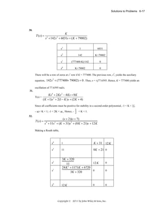
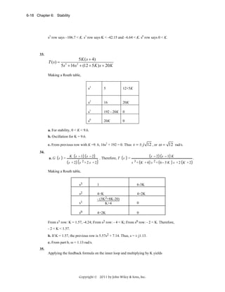
![Solutions to Problems 6-19
Ge =
K
s( s + 10s + 22)
2
Thus,
T=
K
s + 10s + 22 s + K
3
2
Making a Routh table:
s3
1
22
s2
10
K
s1
220 − K
0
s0
K
0
For oscillation, the s1 row must be a row of zeros. Thus, K = 220 will make the system oscillate. The
previous row now becomes, 10s2 + 220. Thus, s2 + 22 = 0, or s = ± j 22
frequency of oscillation is
22 . Hence, the
22 rad/s.
36.
Ks2 + 2Ks
T(s) = 3
s + (K-1)s2 + (2K-4)s + 24
s3
s2
1
2K-4
K-1
24
s1
2K 2 − 6K − 20
K −1
s0
24
0
0
For stability, K > 5; Row of zeros if K = 5. Therefore, 4s2 + 24 = 0. Hence, ω = 6 for
oscillation.
37.
Program:
K=[0:0.001:200];
for i=1:length(K);
deng=conv([1 -4 8],[1 3]);
numg=[0 K(i) 2*K(i) 0];
dent=numg+deng;
R=roots(dent);
A=real(R);
Copyright © 2011 by John Wiley & Sons, Inc.](https://image.slidesharecdn.com/solutionscontrolsystemsengineeringbynormannice6ed-130502172814-phpapp02-131105052456-phpapp01/85/Solutions-control-system-sengineering-by-normannice-6ed-130502172814-phpapp02-316-320.jpg)
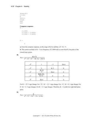
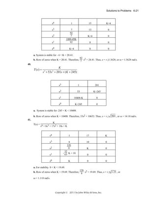
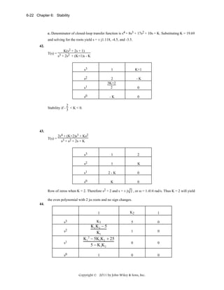
![6-26 Chapter 6: Stability
The second row of zeros was substituted with the coefficients resulting from differentiating the
2
K 2 Kω 0
)s +
characteristic equation: Qa ( s ) = s + (aω +
and
mT
mT
K
2
Q' a ( s) = 4s 3 + 2(aω 0 +
).
mT
4
2
0
Since all the plant parameters are positive, there are two sign changes in the first column of the
Routh array. So there are two poles in the RHP, two must be in the LHP.
49.
The characteristic equation for the system is 1 +
complex conjugate poles at s = ± j
K
K
= 0 or s 2 +
= 0 . The system has two
2
Ib
Ibs
K
. The arm will oscillate at a frequency
Ib
K
rad/sec.
Ib
50.
Eigenvalues are the roots of the following equation:
⎡ s 0 0⎤ ⎡ 0 1
−1
−3 ⎤
3⎤ ⎡s
⎢
⎥ ⎢
⎥ ⎢
⎥
3
2
4 ⎥ = s − 5s − 15s + 40
sI − A = ⎢ 0 s 0⎥ − ⎢ 2 2 −4⎥ = ⎢ −2 s − 2
⎢
⎥ ⎢
⎥ ⎢
⎥
4
s − 3⎦
⎣ 0 0 s⎦ ⎣ 1 −4 3 ⎦ ⎣ −1
Hence, eigenvalues are -3.2824, 1.9133, 6.3691. Therefore, 1 rhp, 2 lhp, 0 jω.
51.
Program:
A=[0 1 0;0 1 -4;-1 1 8];
eig(A)
Computer response:
ans =
7.4641
0.5359
1.0000
52.
Writing the open-loop state and output equations we get,
Copyright © 2011 by John Wiley & Sons, Inc.](https://image.slidesharecdn.com/solutionscontrolsystemsengineeringbynormannice6ed-130502172814-phpapp02-131105052456-phpapp01/85/Solutions-control-system-sengineering-by-normannice-6ed-130502172814-phpapp02-323-320.jpg)
![Solutions to Problems 6-27
•
x1 = x 2
•
x2 = x 2 + 3x 3
•
x3 = −3x1 − 4x 2 − 5x 3 + u
y = x2 + x3
Drawing the signal-flow diagram and including the unity feedback path yields,
1
1
1
1
3
s
1
r
x
1
1
s
1
x
3
s
2
1
-5
-4
-3
-1
Writing the closed-loop state and output equations from the signal-flow diagram,
•
x1 = x 2
•
x2 = x 2 + 3x 3
•
x3 = −3x1 − 4x 2 − 5x 3 + r − c
= −3x1 − 4x 2 − 5x3 + r − (x2 + x3 )
= −3x1 − 5x2 − 6x 3 + r
y = x2 + x3
In vector-matrix form,
⎡0 1 0 ⎤
⎡ 0⎤
x = ⎢ 0 1 3 ⎥ X + ⎢ 0⎥ r
⎢−3 −5 −6 ⎥
⎢ 1⎥
⎣
⎣ ⎦
⎦
•
y = [0 1 1]x
Now, find the characteristic equation.
Copyright © 2011 by John Wiley & Sons, Inc.
x
c=y
1](https://image.slidesharecdn.com/solutionscontrolsystemsengineeringbynormannice6ed-130502172814-phpapp02-131105052456-phpapp01/85/Solutions-control-system-sengineering-by-normannice-6ed-130502172814-phpapp02-324-320.jpg)
![6-28 Chapter 6: Stability
−1
0 ⎤
⎡ s 0 0⎤ ⎡ 0 1 0 ⎤ ⎡ s
−3 ⎥
sI − A = ⎢0 s 0⎥ − ⎢ 0 1 3 ⎥ = ⎢ 0 (s − 1)
⎢0 0 s⎥ ⎢ −3 −5 −6⎥ ⎢ 3
5`
(s + 6)⎥
⎦ ⎣
⎦
⎣
⎦ ⎣
= s3 + 5s2 + 9s + 9
Forming a Routh table to determine stability
s3
s2
s1
s0
1
5
36
5
9
9
9
0
0
Since there are no sign changes, the closed-loop system is stable.
53.
Program:
A=[0,1,0;0,1,3;-3,-4,-5];
B=[0;0;1];
C=[0,1,1];
D=0;
'G'
G=ss(A,B,C,D)
'T'
T=feedback(G,1)
'Eigenvalues of T'
ssdata(T);
eig(T)
Computer response:
ans =
G
a =
x1
x2
x3
x1
0
0
-3
x2
1
1
-4
x3
0
3
-5
x2
1
x3
1
b =
x1
x2
x3
u1
0
0
1
c =
y1
x1
0
Copyright © 2011 by John Wiley & Sons, Inc.](https://image.slidesharecdn.com/solutionscontrolsystemsengineeringbynormannice6ed-130502172814-phpapp02-131105052456-phpapp01/85/Solutions-control-system-sengineering-by-normannice-6ed-130502172814-phpapp02-325-320.jpg)
![6-34 Chapter 6: Stability
For stability row 2 requires K > −1630 and row 4 requires K > −133.008 . The dominant
requirement being the latter. It is clear also that when K > −133.008 , the first element on row 3 is
positive. So the overall requirement for stability is K > −133.008 .
62.
The characteristic equation of the system is given by:
1+
KC
K
1
− C
= 0 or
ms + bs + k K f Ts + 1
2
K f (ms 2 + bs + k )(Ts + 1) + K f K C (Ts + 1) − K C (ms 2 + bs + k ) = 0 or
K f (ms 2 + bs + k )(Ts + 1) + K f K C (Ts + 1) − K C (ms 2 + bs + k ) = 0 or
K f (mTs 3 + (bT + m) s 2 + (kT + b) s + k ) + K f K C (Ts + 1) − K C (ms 2 + bs + k ) = 0 or
K f mTs 3 + [ K f (bT + m) − K C m]s 2 + [ K f (kT + b) + K f K C T − K C b]s + [k + K f K C − K C k ] = 0
Substituting numerical values the equation becomes:
5.28 × 10 −6 K f s 3 + [0.03444 K f − 1.8]s 2 + [1584.78 K f − 11700]s + [22500 K f − 31.5 × 10 6 ] = 0
The Routh array is given by
s3
5.28 × 10 −6 K f
s2
0 . 03444
s
5.28 × 10 −6 22500 K f − 31.5 × 10 6 − 1584.78 K f − 11700 0.03444 K f − 1.8
1
[
K
1584.78K f − 11700
f
− 1 .8
[
] [
]
][
− 0.03444 K f − 1.8
22500 K f − 31.5 × 10 6
To obtain positive quantities on the first column it is required:
5.28 × 10 −6 K f > 0 ⇒ K f > 0
0.03444 K f − 1.8 > 0 ⇒ K f > 52.26
22500 K f − 31.5 × 10 6 > 0 ⇒ K f > 1400
Copyright © 2011 by John Wiley & Sons, Inc.
]
22500 K f − 31.5 × 10 6](https://image.slidesharecdn.com/solutionscontrolsystemsengineeringbynormannice6ed-130502172814-phpapp02-131105052456-phpapp01/85/Solutions-control-system-sengineering-by-normannice-6ed-130502172814-phpapp02-331-320.jpg)
![Solutions to Design Problems 6-35
[1584.78K
f
][
]
[
]
− 11700 0.03444 K f − 1.8 − 5.28 × 10 −6 22500 K f − 31.5 × 10 6 > 0
or
54.52 K 2 − 402.48 K f − 2852.6 K f + 21060 > 0.1188 K 2 − 166.32 K f
f
f
or
54.4 K 2 − 3088.76 K f + 21060 > 0
f
or
K 2 − 56.8 K f + 387.1 > 0
f
or
( K f − 7.92)( K f − 48.88) > 0
So either
or
K f < 7.92 and K f < 48.88 ⇒ K f < 7.92
K f > 7.92 and K f > 48.88 ⇒ K f > 7.92
The most dominant requirement is given by the fourth row. We conclude requiring
K f > 1400 .
63.
a. The Mesh equations obtained by defining clockwise mesh currents are given by
I1 :
I2 :
I3 :
1
+ R) I 1 − RI 2 = V1
sC
1
− RI 1 + (2 R +
) I 2 − RI 3 = 0
sC
1
− RI 2 + (2 R +
)I 3 = 0
sC
(
Solving for I 3 ,
Copyright © 2011 by John Wiley & Sons, Inc.](https://image.slidesharecdn.com/solutionscontrolsystemsengineeringbynormannice6ed-130502172814-phpapp02-131105052456-phpapp01/85/Solutions-control-system-sengineering-by-normannice-6ed-130502172814-phpapp02-332-320.jpg)
![Solutions to Design Problems 6-39
s5
250
213
s4
335
45.5 + 4 K
0
0.5
0
335(3.5 + K ) − 125
0
C
0.5
0
C [335 (3.5 + K ) − 125] − 0.5 × [335 × 213 − 250 × (45.5 + 4 K )]
C
0
335 × 213 − 250 × (45.5 + 4Κ ) #
s3
s2
s1
3.5 + K
s0
0.5
From the s3 row:
335 × 213 − 250 × (45.5 + 4Κ ) > 0 , therefore K < 59.98
(4)
From the s2 row: C =
[335 × 213 − 250(45.5 + 4 K )]× (45.5 + 4 K ) − 335 × [335(3.5 + K ) − 125] > 0.
335 × 213 − 250(45.5 + 4 K )
Therefore:
[335 × 213 − 250(45.5 + 4 K )]× (45.5 + 4 K ) − 335 × [335(3.5 + K ) − 125] > 0.
This inequality may be expanded to:
[59980 − 1000K ]× (45.5 + 4 K ) − 112225K − 392787.5 + 41875 =
− 4000 K 2 + 82195 K + 2378177.5 > 0 , or ( K − 36.7339) × ( K + 16.1852) < 0 which
shows that for stability:
K < 36.73
For C > 0, the s1 row
C [335 (3.5 + K ) − 125] − 0.5 × [335 × 213 − 250 × (45.5 + 4 K )]
is
C
greater than 0 if:
#
3
1
The S row was multiplied by 335 and the S row was multiplied by C.
Copyright © 2011 by John Wiley & Sons, Inc.](https://image.slidesharecdn.com/solutionscontrolsystemsengineeringbynormannice6ed-130502172814-phpapp02-131105052456-phpapp01/85/Solutions-control-system-sengineering-by-normannice-6ed-130502172814-phpapp02-336-320.jpg)
![6-40 Chapter 6: Stability
[335 (3.5 + K ) − 125] − 0.5 × [335 × 213 − 250 × (45.5 + 4 K )] > 0
C
This inequality may be re-written as:
[335 (3.5 + K ) − 125] −
0.5 × [335 × 213 − 250 × (45.5 + 4 K )]2
[335 × 213 − 250(45.5 + 4 K )]× (45.5 + 4 K ) − 335 × [335(3.5 + K ) − 125]
>0
After algebraic manipulations this can be rewritten as:
−1340000 K 3 + 22845325K 2 + 942768725 K + 6.9234 ×10⁸ > 0
or
( K + 0.7485)( K + 18.84)( K − 36.7) < 0
From the previous, and for positive K, we conclude that the system will be stable only if level
controller’s derivative gain, KDLC is within the range: 0 < KDLC< 36.7.
66.
⎡ s + 11.7 − 6.8 − 61.6 K
⎢ 3.5
s + 24 66.9 K
sI − A = ⎢
⎢ 0
−1
s
⎢
0
10
⎣ −1
− 7.7 K ⎤
− 8.4 K ⎥
⎥
0 ⎥
⎥
s ⎦
s + 24 66.9 K − 8.4 K
det( sI − A ) = ( s + 11.7) − 1
0
3.5 66.9 K
− 61.6 K 0
−1
−1
0
− 8.4 K
0
s
s
0
10
s
3.5 66.9 K
+ 6.8 0
−1
3.5 s + 24 66.9 K
+ 7.7 K 0
−1
s
−1
0
10
Copyright © 2011 by John Wiley & Sons, Inc.
s
10
− 8.4 K
0
s](https://image.slidesharecdn.com/solutionscontrolsystemsengineeringbynormannice6ed-130502172814-phpapp02-131105052456-phpapp01/85/Solutions-control-system-sengineering-by-normannice-6ed-130502172814-phpapp02-337-320.jpg)
![6-44 Chapter 6: Stability
2.491 ( K P s + 40 ) ( s + 0.6 )
Ω ( s)
=
2
Rv ( s) s 6 s + 3.613 s + 0.0572 + 0.11035 K P s 2 + (40 + 0.6 K P ) s + 24
(
[
)
=
]
2.491( KPs + 40 ) (s + 0.6 )
6s + ( 3.613 + 0.11035KP ) s2 +( 4.4712 + 0.06621KP ) s + 2.65
3
Noting that the change in car speed, v =
r
itot
ω = 0.06154 ω , we get the system transfer function, T(s) =
V(s)/Rv(s):
0.1533 ( s + 40 ) ( s + 0.6 )
V ( s)
Ω (s)
= 0.06154
=
3
Rv ( s )
Rv ( s )
6 s + ( 3.613 + 0.11035 K P ) s 2 + ( 4.4712 + 0.06621 K P ) s + 2.65
The characteristic polynomial for that system is, therefore:
P(s) = 6 s 3 + (3.613 + 0.11035 K P ) s 2 + (4.4712 + 0.06621 K P ) s + 2.65
Hence, the Routh-Hurwitz for the system is given by:
s3
6
4.4712 + 0.06621 K P
0
s2
3.613 + 0.11035 K P
2.65
0
s1
(3.613 + 0.11035 K P )(4.4712 + 0.06621 K P ) − 15.9
0
0
0
0
3.613 + 0.11035 K P
s0
2.65
For stability,
3.613 + 0.11035 K P ≥ 0 ⇒ K P ≥ −32.74 and
Copyright © 2011 by John Wiley & Sons, Inc.](https://image.slidesharecdn.com/solutionscontrolsystemsengineeringbynormannice6ed-130502172814-phpapp02-131105052456-phpapp01/85/Solutions-control-system-sengineering-by-normannice-6ed-130502172814-phpapp02-341-320.jpg)
![7-2 Chapter 7: Steady-State Errors
s3
1
2x10⁵
s2
2x10⁴
1.2x10⁸
s1
194000
0
s0
120000000
0
we see that the system is stable.
c.
Program:
numg=200000*[1 600];
deng=poly([0 0 -20000]);
G=tf(numg,deng);
'T(s)'
T=feedback(G,1)
poles=pole(T)
Computer response:
ans =
T(s)
Transfer function:
200000 s + 1.2e008
-----------------------------------s^3 + 20000 s^2 + 200000 s + 1.2e008
poles =
1.0e+004 *
-1.9990
-0.0005 + 0.0077i
-0.0005 - 0.0077I
ANSWERS TO REVIEW QUESTIONS
1. Nonlinear, system configuration
2. Infinite
3. Step(position), ramp(velocity), parabola(acceleration)
4. Step(position)-1, ramp(velocity)-2, parabola(acceleration)-3
5. Decreases the steady-state error
6. Static error coefficient is much greater than unity.
7. They are exact reciprocals.
8. A test input of a step is used; the system has no integrations in the forward path; the error for a step input
is 1/10001.
9. The number of pure integrations in the forward path
Copyright © 2011 by John Wiley & Sons, Inc.](https://image.slidesharecdn.com/solutionscontrolsystemsengineeringbynormannice6ed-130502172814-phpapp02-131105052456-phpapp01/85/Solutions-control-system-sengineering-by-normannice-6ed-130502172814-phpapp02-344-320.jpg)

![Solutions to Problems 7-11
e. Poles of T(s) = -3.0190, -1.3166, 0.3426 ± j0.7762, -0.3495. Therefore, system is unstable and
results of (c) and (d) are meaningless
33.
a. For the inner loop:
10
s(s+1)(s+3)(s+4)
10
= 3 2
G1(s) =
20
s(s +8s +19s+32)
1 + (s+1)(s+3)(s+4)
Ge(s) =
20
s(s3+8s2+19s+32)
Ge(s)
20
T(s) = 1+G (s) = 4 3
s +8s +19s2+32s+20
e
b. From Ge(s), system is Type 1.
c. Since system is Type 1, ess = 0
20 5
5
d. From Ge(s), Kv = lim sGe (s) = 32 = 8 . Therefore, ess = K = 8.
v
s→ 0
e. Poles of T(s) = -5.4755, -0.7622 ± j1.7526, -1. Therefore, system is stable and results of parts c and
d are valid.
34.
Program:
numg1=[1 9];deng1=poly([0 -6 -12 -14]);
'G1(s)='
G1=tf(numg1,deng1)
numg2=6*poly([-9 -17]);deng2=poly([-12 -32 -68]);
'G2(s)='
G2=tf(numg2,deng2)
numh1=13;denh1=1;
'H1(s)='
H1=tf(numh1,denh1)
numh2=1;denh2=[1 7];
'H2(s)='
H2=tf(numh2,denh2)
%Close loop with H1 and form G3
'G3(s)=G2(s)/(1+G2(s)H1(s)'
G3=feedback(G2,H1)
%Form G4=G1G3
'G4(s)=G1(s)G3(s)'
G4=series(G1,G3)
%Form Ge=G4/1+G4H2
'Ge(s)=G4(s)/(1+G4(s)H2(s))'
Ge=feedback(G4,H2)
%Form T(s)=Ge(s)/(1+Ge(s)) to test stability
'T(s)=Ge(s)/(1+Ge(s))'
T=feedback(Ge,1)
'Poles of T(s)'
pole(T)
%Computer response shows that system is stable. Now find error specs.
Kp=dcgain(Ge)
'sGe(s)='
sGe=tf([1 0],1)*Ge;
'sGe(s)'
Copyright © 2011 by John Wiley & Sons, Inc.](https://image.slidesharecdn.com/solutionscontrolsystemsengineeringbynormannice6ed-130502172814-phpapp02-131105052456-phpapp01/85/Solutions-control-system-sengineering-by-normannice-6ed-130502172814-phpapp02-353-320.jpg)
![7-12 Chapter 7: Steady-State Errors
sGe=minreal(sGe)
Kv=dcgain(sGe)
's^2Ge(s)='
s2Ge=tf([1 0],1)*sGe;
's^2Ge(s)'
s2Ge=minreal(s2Ge)
Ka=dcgain(s2Ge)
essstep=100/(1+Kp)
essramp=100/Kv
essparabola=200/Ka
Computer response:
ans =
G1(s)=
Transfer function:
s + 9
------------------------------s^4 + 32 s^3 + 324 s^2 + 1008 s
ans =
G2(s)=
Transfer function:
6 s^2 + 156 s + 918
-----------------------------s^3 + 112 s^2 + 3376 s + 26112
ans =
H1(s)=
Transfer function:
13
ans =
H2(s)=
Transfer function:
1
----s + 7
ans =
G3(s)=G2(s)/(1+G2(s)H1(s)
Transfer function:
6 s^2 + 156 s + 918
-----------------------------s^3 + 190 s^2 + 5404 s + 38046
Solutions to Problems 7-13
ans =
G4(s)=G1(s)G3(s)
Transfer function:
6 s^3 + 210 s^2 + 2322 s + 8262
-----------------------------------------------------s^7 + 222 s^6 + 11808 s^5 + 273542 s^4 + 3.16e006 s^3
+ 1.777e007 s^2 + 3.835e007 s
ans =
Ge(s)=G4(s)/(1+G4(s)H2(s))
Transfer function:
6 s^4 + 252 s^3 + 3792 s^2 + 24516 s + 57834
------------------------------------------------------s^8 + 229 s^7 + 13362 s^6 + 356198 s^5 + 5.075e006 s^4
+ 3.989e007 s^3 + 1.628e008 s^2 + 2.685e008 s
+ 8262
ans =
T(s)=Ge(s)/(1+Ge(s))
Transfer function:
6 s^4 + 252 s^3 + 3792 s^2 + 24516 s + 57834
------------------------------------------------------s^8 + 229 s^7 + 13362 s^6 + 356198 s^5 + 5.075e006 s^4
+ 3.989e007 s^3 + 1.628e008 s^2 + 2.685e008 s
+ 66096
ans =
Poles of T(s)
ans =
-157.1538
-21.6791
Copyright © 2011 by John Wiley & Sons, Inc.](https://image.slidesharecdn.com/solutionscontrolsystemsengineeringbynormannice6ed-130502172814-phpapp02-131105052456-phpapp01/85/Solutions-control-system-sengineering-by-normannice-6ed-130502172814-phpapp02-354-320.jpg)
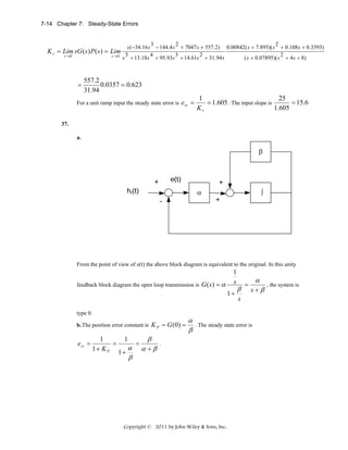
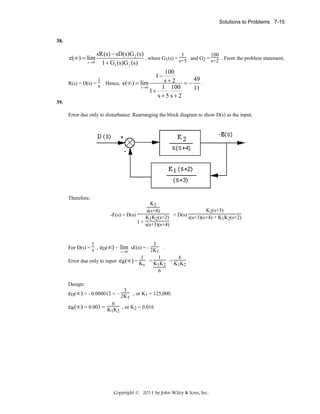
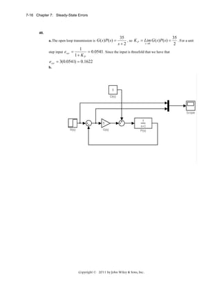
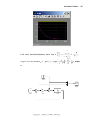
![7-24 Chapter 7: Steady-State Errors
s0
4K
0
0
Therefore, system is stable for 0 < K and steady-state error calculations are valid.
46.
Program:
K=10
numg1=K*poly([-1 -2]);deng1=poly([0 0 -4 -5 -6]);
'G1(s)='
G1=tf(numg1,deng1)
numh1=[1 6];denh1=poly([-8 -9]);
'H1(s)='
H1=tf(numh1,denh1)
'H2(s)=H1-1'
H2=H1-1
%Form Ge(s)=G1(s)/(1+G1(s)H2(s)
'Ge(s)=G1(s)/(1+G1(s)H2(s))'
Ge=feedback(G1,H2)
%Test system stability
'T(s)=Ge(s)/(1+Ge(s))'
T=feedback(Ge,1)
pole(T)
Kp=dcgain(Ge)
'sGe(s)'
sGe=tf([1 0],1)*Ge;
sGe=minreal(sGe)
Kv=dcgain(sGe)
's^2Ge(s)'
s2Ge=tf([1 0],1)*sGe;
s2Ge=minreal(s2Ge)
Ka=dcgain(s2Ge)
essstep=30/(1+Kp)
essramp=30/Kv
essparabola=60/Ka
K=1E6
numg1=K*poly([-1 -2]);deng1=poly([0 0 -4 -5 -6]);
'G1(s)='
G1=tf(numg1,deng1)
numh1=[1 6];denh1=poly([-8 -9]);
'H1(s)='
H1=tf(numh1,denh1)
'H2(s)=H1-1'
H2=H1-1
%Form Ge(s)=G1(s)/(1+G1(s)H2(s)
'Ge(s)=G1(s)/(1+G1(s)H2(s))'
Ge=feedback(G1,H2)
%Test system stability
'T(s)=Ge(s)/(1+Ge(s))'
T=feedback(Ge,1)
pole(T)
Kp=dcgain(Ge)
'sGe(s)'
sGe=tf([1 0],1)*Ge;
sGe=minreal(sGe)
Copyright © 2011 by John Wiley & Sons, Inc.](https://image.slidesharecdn.com/solutionscontrolsystemsengineeringbynormannice6ed-130502172814-phpapp02-131105052456-phpapp01/85/Solutions-control-system-sengineering-by-normannice-6ed-130502172814-phpapp02-366-320.jpg)
![Solutions to Problems 7-25
Kv=dcgain(sGe)
's^2Ge(s)'
s2Ge=tf([1 0],1)*sGe;
s2Ge=minreal(s2Ge)
Ka=dcgain(s2Ge)
essstep=30/(1+Kp)
essramp=30/Kv
essparabola=60/Ka
Computer response:
K =
10
ans =
G1(s)=
Transfer function:
10 s^2 + 30 s + 20
------------------------------s^5 + 15 s^4 + 74 s^3 + 120 s^2
ans =
H1(s)=
Transfer function:
s + 6
--------------s^2 + 17 s + 72
ans =
H2(s)=H1-1
Transfer function:
-s^2 - 16 s - 66
---------------s^2 + 17 s + 72
ans =
Ge(s)=G1(s)/(1+G1(s)H2(s))
Transfer function:
10 s^4 + 200 s^3 + 1250 s^2 + 2500 s + 1440
----------------------------------------------------------------------s^7 + 32 s^6 + 401 s^5 + 2448 s^4 + 7178 s^3 + 7480 s^2 - 2300 s - 1320
Copyright © 2011 by John Wiley & Sons, Inc.](https://image.slidesharecdn.com/solutionscontrolsystemsengineeringbynormannice6ed-130502172814-phpapp02-131105052456-phpapp01/85/Solutions-control-system-sengineering-by-normannice-6ed-130502172814-phpapp02-367-320.jpg)
![Solutions to Problems 7-29
- 2.3e008 s - 1.32e008
Ka =
0
essstep =
-330.0000
essramp =
Inf
essparabola =
Inf
47.
a. Mason’s rule can be used to find the open loop transfer from input to output:
Only one forward path,
T1 = K T ( K v +
1
1
)K m
τs
LCs 2
K mα
Three touching loops,
Ls
K α
1
1
Δ = 1+ m +
+
Ls
LCs 2 Z L Cs
L1 = −
,
L2 = −
1
1
, L3 = −
2
Z L Cs
LCs
; Δ1 = 1
KT K m
1
(K v + )
2
TΔ
1
τs
LCs
. Letting Z L =
G ( s) = 1 1 =
K α
1
1
sC L
Δ
1+ m +
+
2
Ls
LCs
Z L Cs
KT K m
1
(K v + )
2
K K ( K τs + 1)
τs
LCs
= 2 T m v
G(s) =
K α
C
1
τs [L(C + C L ) s + K mαC ]
1+ m +
+ L
2
Ls
C
LCs
Since the system is not unity feedback, we calculate
K T K m ( K vτs + 1)
τs [L(C + C L ) s + K mαC ]
G ( s)
=
K K ( K τs + 1)
K K ( K τs + 1)
1 + GH ( s ) − G ( s )
1+ β 2 T m v
− 2 T m v
τs [L(C + C L ) s + K mαC ] τs [L(C + C L ) s + K mαC ]
( K vτs + 1)
K K
= T m
K K
τ
s 2 [L(C + C L ) s + K mαC ] + ( β − 1) T m ( K vτs + 1)
2
τ
Copyright © 2011 by John Wiley & Sons, Inc.](https://image.slidesharecdn.com/solutionscontrolsystemsengineeringbynormannice6ed-130502172814-phpapp02-131105052456-phpapp01/85/Solutions-control-system-sengineering-by-normannice-6ed-130502172814-phpapp02-371-320.jpg)
![7-30 Chapter 7: Steady-State Errors
The system is type 0.
b. For a step input we calculate K P = Lim
s →0
Then
ess =
1
G(s)
=
1 + GH ( s ) − G ( s ) β − 1
1
1
= 1−
1+ KP
β
48.
G1(s)G2(s)
D(s)G2(s)
Y(s) = R(s) 1 + G (s)G (s)H(s) + 1 + G (s)G (s)H(s)
1
2
1
2
G1(s)G2(s)
D(s)G2(s)
E(s) = R(s) - Y(s) = R(s) - 1 + G (s)G (s)H(s) R(s) - 1 + G (s)G (s)H(s)
1
2
1
2
G1(s)G2(s)
G2(s)
= ⎡1 - 1 + G (s)G (s)H(s)⎤ R(s) - 1 + G (s)G (s)H(s) D(s)
1
2
1
2
⎣
⎦
Thus,
⎧⎡
⎫
⎤
G1 (s)G 2 (s)
G 2 (s)
⎪
⎪
e(∞) = lim sE(s) = lim ⎨ ⎢1 −
⎥ R(s) − 1 + G (s)G (s)H(s) D(s) ⎬
s→0
s→0
⎪ ⎣ 1 + G1 (s)G 2 (s)H(s) ⎦
⎪
1
2
⎩
⎭
49.
a. E(s) = R(s) - C(s). But, C(s) = [R(s) - C(s)H(s)]G1(s)G2(s) + D(s). Solving for C(s),
R(s)G1(s)G2(s)
D(s)
C(s) = 1 + G (s)G (s)H(s) + 1 + G (s)G (s)H(s)
1
2
1
2
Substituting into E(s),
G1(s)G2(s)
1
E(s) = ⎡1 - 1 + G (s)G (s)H(s)⎤ R(s) - 1 + G (s)G (s)H(s) D(s)
1
2
1
2
⎣
⎦
1
b. For R(s) = D(s) = s ,
e(∞) = lim sE(s) = 1 −
s→0
lim G1 (s)G 2 (s)
1
1 + lim G1 (s)G 2 (s)H(s) 1 + lim G1 (s)G 2 (s)H(s)
s→0
s→0
−
s→0
c. Zero error if G1(s) and/or G2(s) is Type 1. Also, H(s) is Type 0 with unity dc gain.
50.
First find the forward transfer function of an equivalent unity feedback system.
Copyright © 2011 by John Wiley & Sons, Inc.](https://image.slidesharecdn.com/solutionscontrolsystemsengineeringbynormannice6ed-130502172814-phpapp02-131105052456-phpapp01/85/Solutions-control-system-sengineering-by-normannice-6ed-130502172814-phpapp02-372-320.jpg)
![Solutions to Problems 7-41
s3
1
48500 K P
s2
2.89
140165 K P − 584.21
2.89
584.021
s
48500 K P
1
The dominant requirement is given by the third row K P > 0.00417
67.
a.
Yh-Ycat
Spring
displacement
Desired
force
Input
voltage+
1
100
Input
transducer
K
1
1000
Controller
F up
0.7883( s + 53.85)
( s2 + 15.47 s + 9283 )( s 2 + 8.119 s + 376 .3)
Actuator
82300
F out
Pantograph
dynamics
Spring
1
100
Sensor
Y h-Ycat
Spring
displacement
Desired
force
+
K
100
1
1000
Controller
Actuator
Fup
0.7883( s + 53.85)
(s 2 + 15.47s + 9283 )(s 2 + 8.119 s + 376 .3)
82300
-
b.
G(s) =
Pantograph
dynamics
Spring
0.7883(s + 53.85)
Yh (s) − Ycat (s)
= 2
2
Fup (s)
(s + 15.47s + 9283)(s + 8.119s + 376.3)
Ge(s) = (K/100)*(1/1000)*G(s)*82.3e3
0.6488K (s+53.85)
Ge(s) =
(s2 + 8.119s + 376.3) (s2 + 15.47s + 9283)
Kp = 0.6488K*53.85/[(376.3)(9283)] = K*1.0002E-5
Copyright © 2011 by John Wiley & Sons, Inc.
Fout](https://image.slidesharecdn.com/solutionscontrolsystemsengineeringbynormannice6ed-130502172814-phpapp02-131105052456-phpapp01/85/Solutions-control-system-sengineering-by-normannice-6ed-130502172814-phpapp02-383-320.jpg)
![Solutions to Problems 7-43
G ( s) =
0.11 ( s + 0.6) × (100s + K I
SC
)
s [s ( s + 0.5173) + 5 (s + 0.6) × (s + 0.01908) ]
(3)
For the steady-state error for a unit-ramp input, r(t) = t u(t), to be equal to 2.5%:
eramp (∞) =
1
=
lim s G ( s)
s →0
1
0.11 ( s + 0.6) × (100s + K I
)
⎛
SC
lim s ⎜
s → 0 ⎜ s[s ( s + 0.5173) + 5 (s + 0.6) × (s + 0.01908)]
⎝
From equation (4), we get:
1
0.11× 0.6 × K I
⎞
⎟
⎟
⎠
= 0.025 (4)
= 0.025 , which yields: KISC = 34.7.
SC
0 + 5 × 0.6 × 0.01908
c. We’ll start by finding G1(s), the equivalent transfer function of the parallel combination,
representing the torque and speed controllers, shown in Figure P7.35:
G1 ( s ) =
13.53 s 3 ( s + 0.6) ⎛ 100 s + 40 ⎞ 313.53 s 2 + 300 s + 72
(5)
+
⎜
⎟=
( s + 0.5) ( s + 0.5) ⎝
s
s ( s + 0.5)
⎠
Given that the equivalent transfer function of the car is: G2 ( s ) =
6.13 × 10 −3
, we apply equation
s + 0.01908
7.62* of the text taking into consideration that the disturbance here is a step with a magnitude equal to
83.7:
83.7
e( ∞ ) = −
lim
s →0
1
+ lim G1 ( s )
G2 ( s ) s→0
=−
83.7
=0
3.11 + ∞
Copyright © 2011 by John Wiley & Sons, Inc.](https://image.slidesharecdn.com/solutionscontrolsystemsengineeringbynormannice6ed-130502172814-phpapp02-131105052456-phpapp01/85/Solutions-control-system-sengineering-by-normannice-6ed-130502172814-phpapp02-385-320.jpg)
![E I G H T
Root Locus Techniques
SOLUTIONS TO CASE STUDIES CHALLENGES
Antenna Control: Transient Design via Gain
a. From the Chapter 5 Case Study Challenge:
76.39K
s(s+150)(s+1.32)
1
Since Ts = 8 seconds, we search along - , the real part of poles with this settling time, for 180o.
2
G(s) =
We find the point to be - 0.5+j6.9 with 76.39K = 7194.23, or K = 94.18. Second-order
approximation is OK since third pole is much more than 5 times further from the imaginary axis
than the dominant second-order pair.
b.
Program:
numg= 1;
deng=poly([0 -150 -1.32]);
'G(s)'
G=tf(numg,deng)
rlocus(G)
axis([-2,0,-10,10]);
title(['Root Locus'])
grid on
[K1,p]=rlocfind(G)
K=K1/76.39
Computer response:
ans =
G(s)
Transfer function:
1
----------------------s^3 + 151.3 s^2 + 198 s
Select a point in the graphics window
selected_point =
-0.5034 + 6.3325i
Copyright © 2011 by John Wiley & Sons, Inc.](https://image.slidesharecdn.com/solutionscontrolsystemsengineeringbynormannice6ed-130502172814-phpapp02-131105052456-phpapp01/85/Solutions-control-system-sengineering-by-normannice-6ed-130502172814-phpapp02-386-320.jpg)
![Solutions to Case Studies Challenges 8-3
UFSS Vehicle: Transient Design via Gain
a. Push -K1 to the right past the summing junction yielding G(s) =
K(s+0.437)
, where
s(s+2)(s+1.29)(s+0.193)
K = 0.25K1. Combine the parallel feedback paths and obtain H(s) = (s+1). Hence, G(s)H(s) =
K(s+0.437)(s+1)
. The root locus is shown below in (b). Searching the 10% overshoot line (ζ
s(s+2)(s+1.29)(s+0.193)
= 0.591; θ = 126.24ο), we find the operating point to be -1.07 ± j1.46 where K = 3.389, or K1 =
13.556.
b.
Program:
numg= [1 0.437];
deng=poly([0 -2 -1.29 -0.193]);
G=tf(numg,deng);
numh=[1 1];
denh=1;
H=tf(numh,denh);
GH=G*H;
rlocus(GH)
pos=(10);
z=-log(pos/100)/sqrt(pi^2+[log(pos/100)]^2);
sgrid(z,0)
title(['Root Locus with ' , num2str(pos), ' Percent Overshoot Line'])
[K,p]=rlocfind(GH);
pause
K1=K/0.25
T=feedback(K*G,H)
Copyright © 2011 by John Wiley & Sons, Inc.](https://image.slidesharecdn.com/solutionscontrolsystemsengineeringbynormannice6ed-130502172814-phpapp02-131105052456-phpapp01/85/Solutions-control-system-sengineering-by-normannice-6ed-130502172814-phpapp02-388-320.jpg)
![8-4 Chapter 8: Root Locus Techniques
T=minreal(T)
step(T)
title(['Step Response for Design of ' , num2str(pos), ' Percent'])
Computer response:
Select a point in the graphics window
selected_point =
-1.0704 + 1.4565i
K1 =
13.5093
Transfer function:
3.377 s + 1.476
--------------------------------------------s^4 + 3.483 s^3 + 6.592 s^2 + 5.351 s + 1.476
Transfer function:
3.377 s + 1.476
--------------------------------------------s^4 + 3.483 s^3 + 6.592 s^2 + 5.351 s + 1.476
Copyright © 2011 by John Wiley & Sons, Inc.](https://image.slidesharecdn.com/solutionscontrolsystemsengineeringbynormannice6ed-130502172814-phpapp02-131105052456-phpapp01/85/Solutions-control-system-sengineering-by-normannice-6ed-130502172814-phpapp02-389-320.jpg)
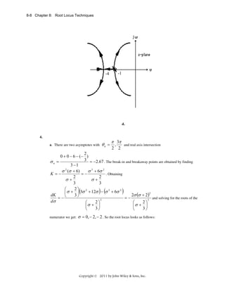
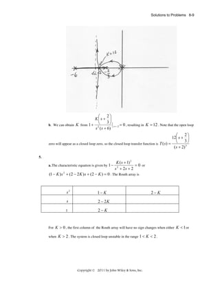
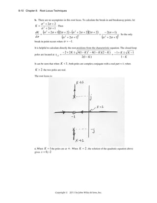
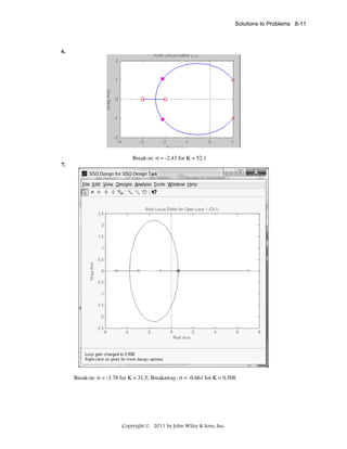
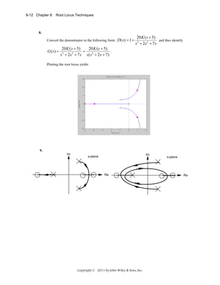
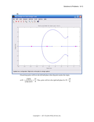
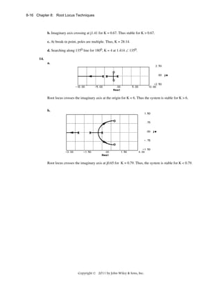
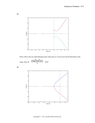
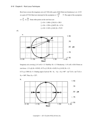

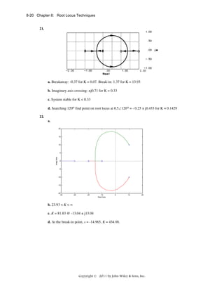
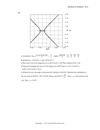
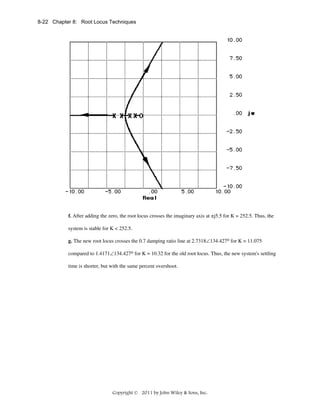
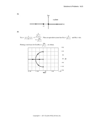
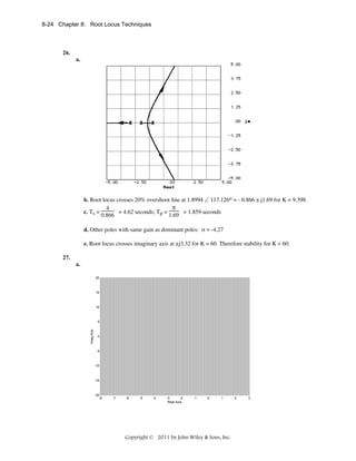
![Solutions to Problems 8-25
b.
a
a
( 6 5 4 2) (2)
4 2
3
(2k 1)
,
4 2
2 2
9.5
c. At the jω axis crossing, K = 115.6. Thus for stability, 0 < K < 115.6.
d. Breakaway points at σ = -2.524 @ K = 0.496 and σ = -5.576 @ K = 0.031.
e. For 25% overshoot, Eq. (4.39) yields ζ = 0.404. Searching along this damping ratio line, we find
the 1800 point at –0.6608 + j1.496 where K = 35.98.
f. –7.839 ± j7.425
g. Second-order approximation not valid because of the existence of closed-loop zeros in the rhp.
h.
Program:
numg=35.98*[1 -2 2];
deng=poly([-2 -4 -5 -6]);
G=tf(numg,deng);
T=feedback(G,1)
step(T)
Computer response:
Transfer function:
35.98 s^2 - 71.96 s + 71.96
-----------------------------------s^4 + 17 s^3 + 140 s^2 + 196 s + 312
Simulation shows over 30% overshoot and nonminimum-phase behavior. Second-order
approximation not valid.
Copyright © 2011 by John Wiley & Sons, Inc.](https://image.slidesharecdn.com/solutionscontrolsystemsengineeringbynormannice6ed-130502172814-phpapp02-131105052456-phpapp01/85/Solutions-control-system-sengineering-by-normannice-6ed-130502172814-phpapp02-410-320.jpg)
![8-28 Chapter 8: Root Locus Techniques
32.
a.
15
10
Imag Axis
5
0
-5
-10
-15
-10
-8
-6
-4
Real Axis
-2
0
2
b. Searching along the 10% overshoot line (angle = 126.239o), the point - 0.7989 + j1.0898 yields
180o for K = 81.74.
c. Higher-order poles are located at approximately –6.318 and –7.084. Since these poles are more than
5 times further from the imaginary axis than the dominant pole found in (b), the second-order
approximation is valid.
d. Searching along the imaginary axis yields 180o at j2.53, with K = 394.2.
Hence, for stability, 0 < K < 394.2.
33.
Program:
pos=10;
z=-log(pos/100)/sqrt(pi^2+[log(pos/100)]^2)
numg=1;
deng=poly([0 -3 -4 -8]);
G=tf(numg,deng)
Gzpk=zpk(G)
rlocus(G,0:1:100)
pause
axis([-2,0,-2,2])
sgrid(z,0)
pause
[K,P]=rlocfind(G)
T=feedback(K*G,1)
pause
step(T)
Computer response:
z =
0.5912
Copyright © 2011 by John Wiley & Sons, Inc.](https://image.slidesharecdn.com/solutionscontrolsystemsengineeringbynormannice6ed-130502172814-phpapp02-131105052456-phpapp01/85/Solutions-control-system-sengineering-by-normannice-6ed-130502172814-phpapp02-413-320.jpg)
![Solutions to Problems 8-31
10
8
6
4
Imag Axis
2
0
-2
-4
-6
-8
-10
-5
-4
-3
-2
-1
0
1
2
Real Axis
b.
Program:
numg=11*[1 4 5];
deng=conv([1 2 5],poly([-3 -4]));
G=tf(numg,deng);
T=feedback(G,1);
step(T)
Peak time approximately 0.8 second instead of 1 second.
Copyright © 2011 by John Wiley & Sons, Inc.](https://image.slidesharecdn.com/solutionscontrolsystemsengineeringbynormannice6ed-130502172814-phpapp02-131105052456-phpapp01/85/Solutions-control-system-sengineering-by-normannice-6ed-130502172814-phpapp02-416-320.jpg)
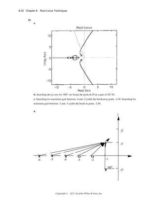
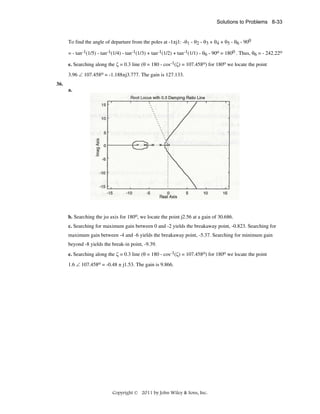
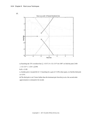
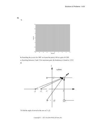
![8-36 Chapter 8: Root Locus Techniques
1
2
3
4
5
6
1
90
0
tan
Solving for θ1, the angle of arrival is θ1 = –191.50.
1
4
3
tan
1
2
4
tan
1
2
5
180
e. The closed-loop zeros are the poles of H(s), or –1 ± j2.
f. Searching the ζ = 0.358; (θ = 110.97ο) for 180o, we find the point
= -0.6537+j1.705. The gain, K = 0.8764.
g. Higher-order poles are at –2.846 ± j1.731. These are not 5 times further than the dominant poles.
Further, there are closed-loop zeros at –1 ± j2 that are not cancelled any higher-order poles. Thus, the
second-order approximation is not valid.
39.
50
40
30
20
Imag Axis
10
0
-10
-20
-30
-40
-50
-40
-35
-30
-25
-20
-15
Real Axis
-10
-5
0
5
a. The root locus crosses the imaginary axis at j2.621 with K = 4365. Therefore, the system is stable
for 0 < K < 4365.
b. Search the 0.707 damping ratio line for 180o and find –0.949 + j0.949 with K = 827.2.
c. Assume critical damping where root locus breaks away from the real axis. Locus breaks away at –
1.104 with K = 527.6.
40.
Program:
numg=1;
deng=poly([0 -3 -7 -8]);
Copyright © 2011 by John Wiley & Sons, Inc.](https://image.slidesharecdn.com/solutionscontrolsystemsengineeringbynormannice6ed-130502172814-phpapp02-131105052456-phpapp01/85/Solutions-control-system-sengineering-by-normannice-6ed-130502172814-phpapp02-421-320.jpg)
![Solutions to Problems 8-37
numh=[1 30];
denh=[1 20 200];
G=tf(numg,deng)
Gzpk=zpk(G)
H=tf(numh,denh)
rlocus(G*H)
pause
K=0:10:1e4;
rlocus(G*H,K)
sgrid(0.707,0)
axis([-2,2,-5,5]);
pause
for i=1:1:3;
[K,P]=rlocfind(G*H)
end
T=feedback(K*G,H)
step(T)
Computer response:
Transfer function:
1
-----------------------------s^4 + 18 s^3 + 101 s^2 + 168 s
Zero/pole/gain:
1
------------------s (s+8) (s+7) (s+3)
Transfer function:
s + 30
---------------s^2 + 20 s + 200
Select a point in the graphics window
selected_point =
-0.9450 + 0.9499i
K =
828.1474
P =
-9.9500
-9.9500
-8.1007
-8.1007
-0.9492
-0.9492
+10.0085i
-10.0085i
+ 1.8579i
- 1.8579i
+ 0.9512i
- 0.9512i
Select a point in the graphics window
selected_point =
0.0103 + 2.6385i
Copyright © 2011 by John Wiley & Sons, Inc.](https://image.slidesharecdn.com/solutionscontrolsystemsengineeringbynormannice6ed-130502172814-phpapp02-131105052456-phpapp01/85/Solutions-control-system-sengineering-by-normannice-6ed-130502172814-phpapp02-422-320.jpg)
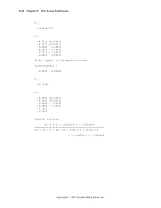
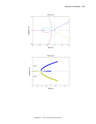
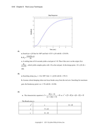
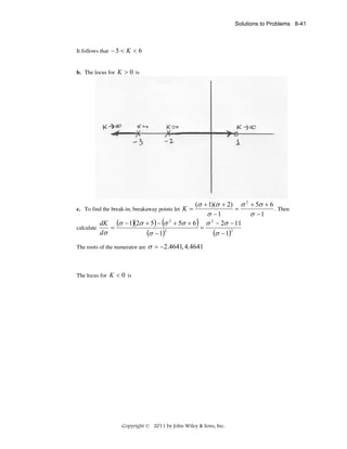
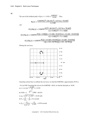
![Solutions to Problems 8-47
c
d
48.
a. Using Figure P8.15(a),
[Ms2+(D+Dc)s+(K+Kc)]X(s) - [Dcs+Kc]Xa(s) = 0
Rearranging,
[Ms2+Ds+K]X(s) = -[Dcs+Kc](X(s)-Xa(s))
(1)
where [Dcs+Kc](X(s)-Xa(s)) can be thought of as the input to the plant.
For the active absorber,
(Mcs2+Dcs+Kc)Xa(s) - (Dcs+Kc)X(s) = 0
or
Mcs2Xa(s)+Dcs(Xa(s)-X(s))+Kc(Xa(s)-X(s)) = 0
Adding -Mcs2X(s) to both sides,
Mcs2(Xa(s)-X(s))+Dcs(Xa(s)-X(s))+Kc(Xa(s)-X(s)) = -Mcs2X(s)
Let Xa(s)-X(s) = Xc(s) and s2X(s) = C(s) = plant output acceleration. Therefore,
Mcs2Xc(s)+DcsXc(s)+KcXc(s) = -McC(s)
or
(Mcs2+Dcs+Kc)Xc(s) = -McC(s)
Using Eqs. (1) and (2), and Xa(s)-X(s) = Xc(s),
Xc(s)
-Mc
Dcs+Kc
X(s)
=
2+D s+K ; Xc(s) = Ms2+Ds+K
C(s)
Mcs
c
c
which suggests the following block diagram:
Copyright © 2011 by John Wiley & Sons, Inc.
(2)](https://image.slidesharecdn.com/solutionscontrolsystemsengineeringbynormannice6ed-130502172814-phpapp02-131105052456-phpapp01/85/Solutions-control-system-sengineering-by-normannice-6ed-130502172814-phpapp02-432-320.jpg)
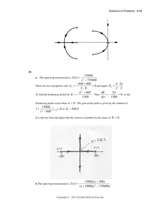
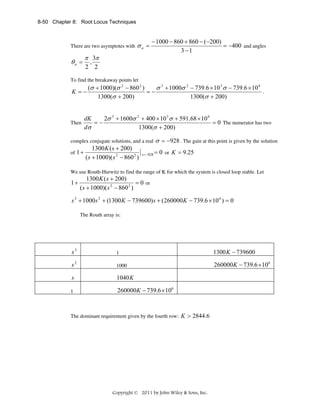
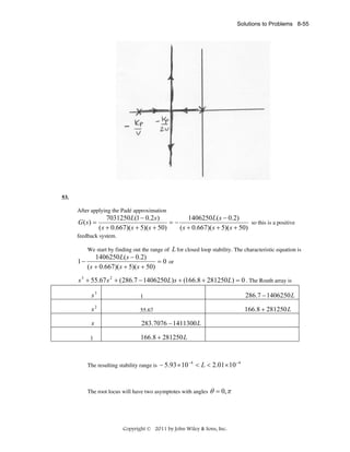
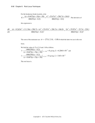
![Solutions to Problems 8-57
54.
a. Using Mason’s rule it can readily be found that (with d=0) the open loop transmission from u r to
u o is
u0
=
ur
(Kν τs + 1)
1 1
K T K m ( Kν τs + 1)
τs
Ls Cs =
C
1
1
τs L(C + C L ) s 2 + K mαCs + 1
1+ Km
α+
+ L
Ls
LCs 2 C
KT
Km
[
So the system’s characteristic equation is:
1+ β
K T K m ( Kν τs + 1)
=0
τs L(C + C L ) s 2 + K mαCs + 1
[
]
or
τL(C + C L ) s 3 + K mαCτs 2 + [τ + βK T K m Kν τ ]s + βK T K m = 0
b. Substituting numerical values the characteristic equation becomes
Copyright © 2011 by John Wiley & Sons, Inc.
]](https://image.slidesharecdn.com/solutionscontrolsystemsengineeringbynormannice6ed-130502172814-phpapp02-131105052456-phpapp01/85/Solutions-control-system-sengineering-by-normannice-6ed-130502172814-phpapp02-442-320.jpg)
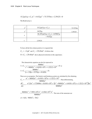
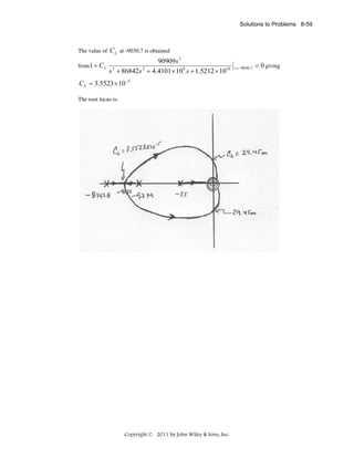
![8-62 Chapter 8: Root Locus Techniques
=
s 2 + 1225s + 2530000
0.008 s 3 + 9.8 s 2 + 40240 s + 500000
b. The transfer function of the forward loop, KG(s):
(
)
Vs ( s )
K s 2 + 1225s + 2530000
KG ( s ) =
=
Ev ( s) 0.008 s 3 + 9.8 s 2 + 40240 s + 500000
The transfer function of the feedback loop is given by: H ( s ) =
200 .
s + 200
The system’s characteristic equation is:
(
)
⎛
⎞⎛ 200 ⎞
K s 2 + 1225s + 2530000
1+ ⎜
3
2
⎜ 0.008 s + 9.8 s + 40240 s + 500000 ⎟⎜ s + 200 ⎟ = 0
⎟
⎠
⎝
⎠⎝
Or equivalently
s 4 + 1425 s 3 + (5275000 + 25000 K )s 2 + (1.0685 × 10⁹ + 3.0625 × 10⁷ K )s + (1.25 ×10¹⁰ + 6.325 ×10¹⁰ K )
=0
The following MATLAB M-file was written to plot the root locus for the system and to find the
required-above operational parameters and functions:
numg = [1 1225 2.53E6];
deng = [0.008 9.8 40240 500000];
G = tf(numg, deng);
numh = 200;
denh = [1 200];
H = tf(numh, denh);
rlocus(G*H);
title('Full Root Locus for DC Bus Voltage Control System')
pause
axis ([-150, 0, -150, 150]);
z=0.707;
sgrid(z,0)
Copyright © 2011 by John Wiley & Sons, Inc.](https://image.slidesharecdn.com/solutionscontrolsystemsengineeringbynormannice6ed-130502172814-phpapp02-131105052456-phpapp01/85/Solutions-control-system-sengineering-by-normannice-6ed-130502172814-phpapp02-447-320.jpg)
![Solutions to Problems 8-63
title('Root Locus Zoomed-in around Dominant Poles with a 0.707
Damping Line')
[K1,p]=rlocfind(G*H);
pause
K = K1;
T=feedback(K*G,H);
%T is the closed-loop TF of the system
T=minreal(T);
step(750*T);
grid
title('Step Response of DC Bus Voltage')
The first figure shown below is the full root locus for that system.
4
1
Full Root Locus for DC Bus Voltage Control System
x 10
T(s)
0.8
0.6
Imaginary Axis
0.4
0.2
0
-0.2
-0.4
-0.6
-0.8
-1
-1200
-1000
-800
-600
-400
-200
0
Real Axis
Copyright © 2011 by John Wiley & Sons, Inc.
200
400
600](https://image.slidesharecdn.com/solutionscontrolsystemsengineeringbynormannice6ed-130502172814-phpapp02-131105052456-phpapp01/85/Solutions-control-system-sengineering-by-normannice-6ed-130502172814-phpapp02-448-320.jpg)
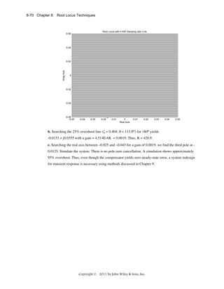
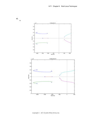
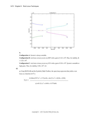
![8-73 Chapter 8: Root Locus Techniques
Program:
syms s N KLSS KHSS KG JR JG tel s
numGdt=3.92*N^2*KLSS*KHSS*KG*s;
denGdt=(N^2*KHSS*(JR*s^2+KLSS)*(JG*s^2*[tel*s+1]+KG*s)+JR*s^2*KLSS*[(JG*s^2
+KHSS)*(tel*s+1)+KG*s]);
Gdt=numGdt/denGdt;
'Gdt in General Terms'
pretty(Gdt)
'Values to Substitute'
KLSS=12.6e6
KHSS=301e3
KG=668
JR=190120
JG=3.8
tel=20e-3
Copyright © 2011 by John Wiley & Sons, Inc.](https://image.slidesharecdn.com/solutionscontrolsystemsengineeringbynormannice6ed-130502172814-phpapp02-131105052456-phpapp01/85/Solutions-control-system-sengineering-by-normannice-6ed-130502172814-phpapp02-458-320.jpg)
![8-74 Chapter 8: Root Locus Techniques
numGdt=3.92*N^2*KLSS*KHSS*KG*s;
numGdt=vpa(numGdt,4);
denGdt=(N^2*KHSS*(JR*s^2+KLSS)*(JG*s^2*[tel*s+1]+KG*s)+JR*s^2*KLSS*[(JG*s^2
+KHSS)*(tel*s+1)+KG*s]);
denGdt=vpa(denGdt,4);
'Gdt with Values Substituted'
Gdt=numGdt/denGdt;
pretty(Gdt)
Gdt=expand(Gdt);
Gdt=vpa(Gdt,4);
'Gdt Different Form 1'
pretty(Gdt);
denGdt=collect(denGdt,N^2);
'Gdt Different Form 2'
Gdt=collect(Gdt,N^2);
pretty(Gdt)
[numGdt,denGdt]=numden(Gdt);
numGdt=numGdt/0.4349e10;
denGdt=denGdt/0.4349e10;
denGdt=expand(denGdt);
denGdt=collect(denGdt,N^2);
Gdt=vpa(numGdt/denGdt,4);
'Gdt Different Form 3'
pretty(Gdt)
'Putting into Form for RL as a Function of N^2 using previous results'
numGH=[1 49.99 8855 3313 582400];
denGH=[41.87 2094 0.3684e7 0.1658e9 0];
denGH=denGH/denGH(1)
GH=tf(numGH,denGH)
GHzpk=zpk(GH)
'Zeros of GH'
rootsnumGH=roots(numGH)
'Poles of GH'
rootsdenGH=roots(denGH)
K=0:1:10000;
rlocus(GH,K)
sgrid(0.5,0)
pause
axis([-10,0,-20,20])
[K,P]=rlocfind(GH)
Computer response:
ans =
Gdt in General Terms
98 2
/
2
2
2
-- N KLSS KHSS KG s / (N KHSS (JR s + KLSS) (JG s (tel s + 1) + KG s)
25
/
2
2
+ JR s KLSS ((JG s + KHSS) (tel s + 1) + KG s))
ans =
Values to Substitute
KLSS =
12600000
Copyright © 2011 by John Wiley & Sons, Inc.](https://image.slidesharecdn.com/solutionscontrolsystemsengineeringbynormannice6ed-130502172814-phpapp02-131105052456-phpapp01/85/Solutions-control-system-sengineering-by-normannice-6ed-130502172814-phpapp02-459-320.jpg)
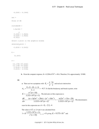
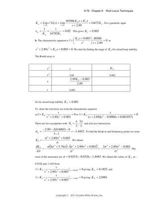
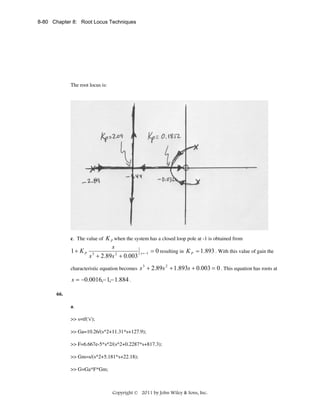
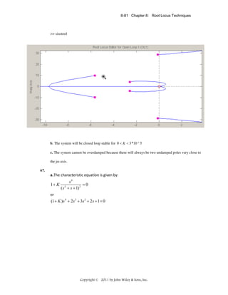
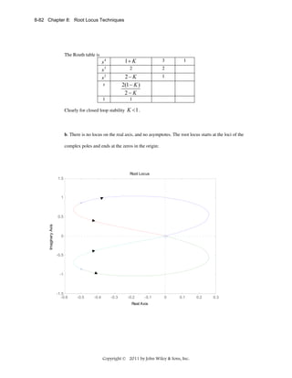
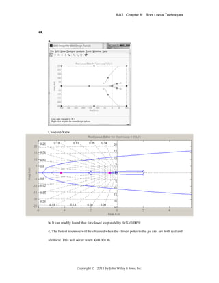
![8-84 Chapter 8: Root Locus Techniques
d. When K=0.00136 the dominant poles are situated at -0.57. The settling time
Ts ≈
4
= 7.02 sec
0.57
e. The actual settling time is 9.7 sec as shown in the figure below.
Step Response
1
0.9
0.8
0.7
Amplitude
0.6
0.5
0.4
0.3
0.2
0.1
0
0
2
4
6
8
10
12
14
16
18
Time (sec)
69.
% Parameters
Jl=10;Bl=1;k=100;Jm=2;Bm=0.5;a=0.25;%a is the location of the zero
%numerator and denominator of the open loop transfer function
numo=k*[1 a];
deno=[Jl*Jm (Jl*Bm+Jm*Bl) (k*(Jl+Jm)+Bl*Bm) k*(Bl+Bm) 0];
syso=tf(numo,deno);
%Pole-Zero map for the open loop transfer function
pzmap(syso);
%Root Locus
rlocus(syso);axis([-1 0 -0.3 0.3]);
zgrid(0.707,[]); %grid for zeta=0.707 for approx. 5% overshoot
[KD,poles]=rlocfind(syso);
%Choose the appropriate location of the poles in the window and multiply the factor by the open
loop
%transfer function
syso=KD*syso;
%Close the loop
sysc=feedback(syso,1);
Copyright © 2011 by John Wiley & Sons, Inc.](https://image.slidesharecdn.com/solutionscontrolsystemsengineeringbynormannice6ed-130502172814-phpapp02-131105052456-phpapp01/85/Solutions-control-system-sengineering-by-normannice-6ed-130502172814-phpapp02-469-320.jpg)
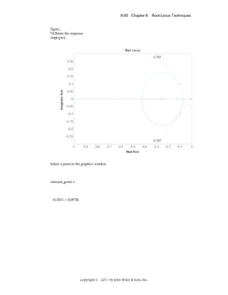
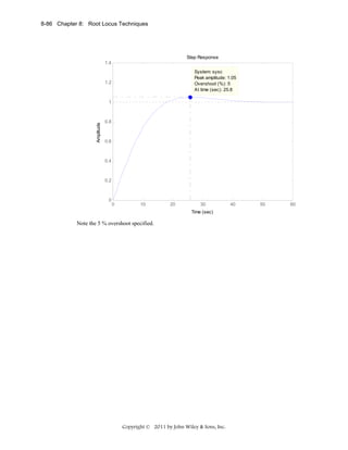
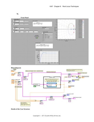
![8-88 Chapter 8: Root Locus Techniques
71.
The following MATLAB M-file was written to plot the root locus for the system and to find the
required-above operational parameters and functions:
numg = poly ([-0.071-6.25i -0.071+6.25i]);
deng = poly ([-0.047 -2 -0.262+5.1i -0.262-5.1i]);
G = tf(numg, deng);
rlocus(G);
pos=(16);
z=-log(pos/100)/sqrt(pi^2+(log(pos/100))^2);
sgrid(z,0)
title(['Root Locus with ', num2str(pos), ' Percent Overshoot Line
for Synchronous Machine with Te = 0.5 sec'])
[K1,p]=rlocfind(G);
pause
K=0.936*K1;
T=feedback(K*G,1);
%T is the closed-loop TF of the system
T=minreal(T);
step(T);
grid
Copyright © 2011 by John Wiley & Sons, Inc.](https://image.slidesharecdn.com/solutionscontrolsystemsengineeringbynormannice6ed-130502172814-phpapp02-131105052456-phpapp01/85/Solutions-control-system-sengineering-by-normannice-6ed-130502172814-phpapp02-473-320.jpg)
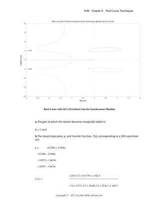
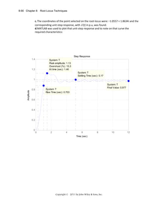
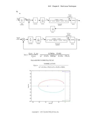

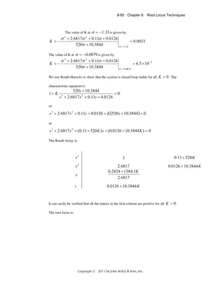
![8-96 Chapter 8: Root Locus Techniques
74.
a.
With the speed controller configured as a proportional controller [KISC= 0 and GSC(s) =
KPSC], the open-loop transfer function is: Gsc (s)Gv ( s) =
0.11 K Psc ( s + 0.6)
s ( s + 0.5173) + 5(s + 0.6)(s + 0.01908)
.
Expanding the denominator of this transfer function, gives:
DG ( s ) = 6 s 2 + 3.613 s + 0.05724 .
Solving for the roots shows that there are two open-loop poles: – 0.5858 and – 0.0163. Thus, the
open-loop transfer function may be re-written as:
Gsc ( s )Gv ( s) =
0.11 K Psc ( s + 0.6)
K1 ( s + 0.6)
=
6s 2 + 3.613 s + 0.05724 ( s + 0.5858)( s + 0.0163)
In this equation: K1 =
K P sc × 0.11
6
(1)
(2)
The following MATLAB M-file was written to plot the root locus for the system and to find the
value of the proportional gain, K1, at the breakaway or break-in points.
Copyright © 2011 by John Wiley & Sons, Inc.](https://image.slidesharecdn.com/solutionscontrolsystemsengineeringbynormannice6ed-130502172814-phpapp02-131105052456-phpapp01/85/Solutions-control-system-sengineering-by-normannice-6ed-130502172814-phpapp02-481-320.jpg)
![8-97 Chapter 8: Root Locus Techniques
numg = [1 0.6];
deng = poly ([-0.0163 -0.5858]);
G = tf(numg, deng);
rlocus(G);
pos=(0);
z=-log(pos/100)/sqrt(pi^2+(log(pos/100))^2);
sgrid(z,0)
title(['Root Locus with ', num2str(pos) , ' Percent Overshoot
Line'])
[K1,p]=rlocfind(G);
pause
T=feedback(K1*G,1);
%T is the closed-loop TF of the system
T=minreal(T);
step(T);
axis ([0, 8, 0, 1]);
grid
The root locus shown below was obtained. Using MATLAB tools, the gain at the break-in point was
found to be larger and, hence, would yield a faster closed-loop unit-step response. The following
repeated real poles were found, which indicated that the step response is critically damped: p = 0.6910, - 0.6910. These poles corresponded to: K1 = 0.78 (which corresponds to KPSC = 42.54). The
closed-loop transfer function, T(s), was found to be:
0.78 s + 0.468
T(s) =
----------------------s2 + 1.382 s + 0.4775
Copyright © 2011 by John Wiley & Sons, Inc.](https://image.slidesharecdn.com/solutionscontrolsystemsengineeringbynormannice6ed-130502172814-phpapp02-131105052456-phpapp01/85/Solutions-control-system-sengineering-by-normannice-6ed-130502172814-phpapp02-482-320.jpg)
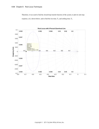
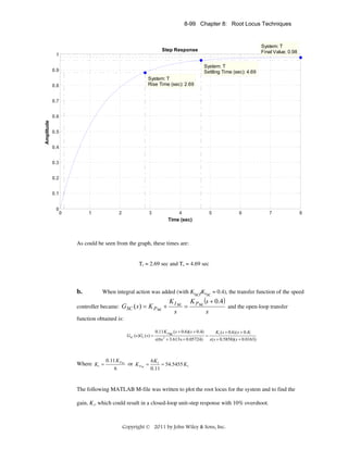
![8-100 Chapter 8: Root Locus Techniques
numg = poly ([-0.4 -0.6]);
deng = poly ([0 -0.0163 -0.5858]);
G = tf(numg, deng);
rlocus(G);
pos=(10);
z=-log(pos/100)/sqrt(pi^2+(log(pos/100))^2);
axis ([-1, 0, -0.5, 0.5]);
sgrid(z,0)
title(['Root Locus with ', num2str(pos) , ' Percent Overshoot
Line'])
[K1,p]=rlocfind(G);
pause
T=feedback(K1*G,1);
%T is the closed-loop TF of the system
T=minreal(T);
step(T);
axis ([0, 20, 0, 1.5]);
grid
The root locus shown below was obtained. Using MATLAB tools, the gain at the point selected on
the locus (- 0.275 + j 0.376) was found to be K1 = 0.526 (which corresponds to KPSC = 28.7). The
corresponding closed-loop transfer function, T(s), is:
T ( s) =
0.526 s 2 + 0.526 s + 0.1262
s 3 + 1.128 s 2 + 0.5355 s + 0.1262
T(s) has the closed-loop poles: p = – 0.580, – 0.275 ± j 0.376 and zeros at – 0.4 & – 0.6. Thus, the
complex conjugate poles are not dominant, and hence, the output response, c(t), obtained using
Copyright © 2011 by John Wiley & Sons, Inc.](https://image.slidesharecdn.com/solutionscontrolsystemsengineeringbynormannice6ed-130502172814-phpapp02-131105052456-phpapp01/85/Solutions-control-system-sengineering-by-normannice-6ed-130502172814-phpapp02-485-320.jpg)
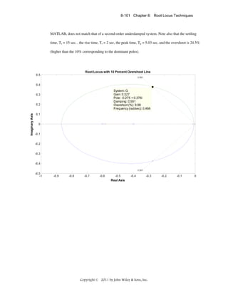

![9-4 Chapter 9: Design via Root Locus
12. 25 times; the improvement equals the ratio of the zero location to the pole location.
13. No; the feedback compensator's zero is not a zero of the closed-loop system.
14. A. Response of inner loops can be separately designed; B. Faster responses possible; C. Amplification
may not be necessary since signal goes from high amplitude to low.
SOLUTIONS TO PROBLEMS
1.
Uncompensated system: Search along the ζ = 0.5 line and find the operating point is at -1.5356 ±
j2.6598 with K = 73.09. Hence, %OS = e
=
− ζπ / 1− ζ
2
x100 = 16.3%; Ts =
4
= 2.6 seconds; Kp
1.5356
73.09
=2.44. A higher-order pole is located at -10.9285.
30
Compensated: Add a pole at the origin and a zero at -0.1 to form a PI controller. Search along the ζ =
0.5 line and find the operating point is at -1.5072 ± j2.6106 with K = 72.23. Hence, the estimated
performance specifications for the compensated system are: %OS = e
− ζπ / 1− ζ
2
x100 = 16.3%; Ts =
4
= 2.65 seconds; Kp = ∞. Higher-order poles are located at -0.0728 and -10.9125. The
1.5072
compensated system should be simulated to ensure effective pole/zero cancellation.
2.
a. Insert a cascade compensator, such as
b.
Program:
K=1
G1=zpk([],[0,-3,-6],K)
Gc=zpk([-0.01],[0],1)
G=G1*Gc
rlocus(G)
T=feedback(G,1)
T1=tf(1,[1,0])
T2=T*T1
t=0:0.1:200;
step(T1,T2,t)
Gc (s) =
s + 0.01
.
s
%G1=1/s(s+3)(s+6)
%Gc=(s+0.01)/s
%Form 1/s to integrate step input
%Show input ramp and ramp response
Computer response:
K =
1
Copyright © 2011 by John Wiley & Sons, Inc.](https://image.slidesharecdn.com/solutionscontrolsystemsengineeringbynormannice6ed-130502172814-phpapp02-131105052456-phpapp01/85/Solutions-control-system-sengineering-by-normannice-6ed-130502172814-phpapp02-491-320.jpg)
![Solutions to Problems 9-7
4.
a. Searching along the 126.16o line (10% overshoot, ζ = 0.59), find the operating point at
-1.1207 + j1.5336 with K = 27.9948. Hence, Kv =
27.9948
= 1.3331 .
3x7
b. A 3.0006 x improvement will yield Kv = 4. Use a lag compensator, Gc(s) =
c.
Program:
K=17.5
G=zpk([],[0,-3,-5],K)
Gc=zpk([-0.3429],[-0.1],1)
Ge=G*Gc;
T1=feedback(G,1);
T2=feedback(Ge,1);
T3=tf(1,[1,0]);
%Form 1/s to integrate step input
T4=T1*T3;
T5=T2*T3;
t=0:0.1:20;
step(T3,T4,T5,t)
%Show input ramp and ramp responses
Computer response:
K =
27.9948
Zero/pole/gain:
27.9948
------------s (s+3) (s+7)
Zero/pole/gain:
(s+0.3001)
---------(s+0.1)
Copyright © 2011 by John Wiley & Sons, Inc.
s + 0.3.0006
.
s + 0.1](https://image.slidesharecdn.com/solutionscontrolsystemsengineeringbynormannice6ed-130502172814-phpapp02-131105052456-phpapp01/85/Solutions-control-system-sengineering-by-normannice-6ed-130502172814-phpapp02-494-320.jpg)
![9-10 Chapter 9: Design via Root Locus
Compensated: To reduce the settling time by a factor of 2, the closed-loop poles should be – 4.64 ±
j4.64. The summation of angles to this point is 119o . Hence, the contribution of the compensating
zero should be 180o -119o =61o . Using the geometry shown below,
4.64
= tan (61o). Or, zc = 7.21.
zc − 4.64
After adding the compensator zero, the gain at -4.64+j4.64 is K = 4.77. Hence,
Kp =
4.77 x 6 x 7.21
4
π
= 6.88 . Ts =
= 0.86 second; Tp =
= 0.677 second;
2 x3 x5
4.64
4.64
%OS = e −ζπ /
1− ζ
2
x100 = 4.33%; ωn =
4.642 + 4.64 2 = 6.56 rad/s; higher-order pole at
-5.49. The problem with the design is that there is steady-state error, and no effective pole/zero
cancellation. The design should be simulated to be sure the transient requirements are met.
7.
Program:
clf
'Uncompensated System'
numg=[1 6];
deng=poly([-2 -3 -5]);
'G(s)'
G=tf(numg,deng);
Gzpk=zpk(G)
rlocus(G,0:1:100)
z=0.707;
pos=exp(-pi*z/sqrt(1-z^2))*100;
sgrid(z,0)
title(['Uncompensated Root Locus with ' , num2str(z), ' Damping Ratio
Line'])
[K,p]=rlocfind(G); %Allows input by selecting point on graphic
'Closed-loop poles = '
p
i=input('Give pole number that is operating point
');
'Summary of estimated specifications'
operatingpoint=p(i)
gain=K
estimated_settling_time=4/abs(real(p(i)))
estimated_peak_time=pi/abs(imag(p(i)))
estimated_percent_overshoot=pos
Copyright © 2011 by John Wiley & Sons, Inc.](https://image.slidesharecdn.com/solutionscontrolsystemsengineeringbynormannice6ed-130502172814-phpapp02-131105052456-phpapp01/85/Solutions-control-system-sengineering-by-normannice-6ed-130502172814-phpapp02-497-320.jpg)
![Solutions to Problems 9-11
estimated_damping_ratio=z
estimated_natural_frequency=sqrt(real(p(i))^2+imag(p(i))^2)
Kp=dcgain(K*G)
'T(s)'
T=feedback(K*G,1)
'Press any key to continue and obtain the step response'
pause
step(T)
title(['Step Response for Uncompensated System with ' , num2str(z),...
' Damping Ratio'])
'Press any key to go to PD compensation'
pause
'Compensated system'
done=1;
while done>0
a=input('Enter a Test PD Compensator, (s+a). a =
')
numc=[1 a];
'Gc(s)'
GGc=tf(conv(numg,numc),deng);
GGczpk=zpk(GGc)
wn=4/[(estimated_settling_time/2)*z];
rlocus(GGc)
sgrid(z,wn)
title(['PD Compensated Root Locus with ' , num2str(z),...
' Damping Ratio Line', 'PD Zero at ', num2str(a), ', and Required Wn'])
done=input('Are you done? (y=0,n=1) ');
end
[K,p]=rlocfind(GGc); %Allows input by selecting point on graphic
'Closed-loop poles = '
p
i=input('Give pole number that is operating point
');
'Summary of estimated specifications'
operatingpoint=p(i)
gain=K
estimated_settling_time=4/abs(real(p(i)))
estimated_peak_time=pi/abs(imag(p(i)))
estimated_percent_overshoot=pos
estimated_damping_ratio=z
estimated_natural_frequency=sqrt(real(p(i))^2+imag(p(i))^2)
Kp=dcgain(K*GGc)
'T(s)'
T=feedback(K*GGc,1)
'Press any key to continue and obtain the step response'
pause
step(T)
title(['Step Response for Compensated System with ' , num2str(z),...
' Damping Ratio'])
Computer response:
ans =
Uncompensated System
ans =
G(s)
Zero/pole/gain:
(s+6)
----------------(s+5) (s+3) (s+2)
Copyright © 2011 by John Wiley & Sons, Inc.](https://image.slidesharecdn.com/solutionscontrolsystemsengineeringbynormannice6ed-130502172814-phpapp02-131105052456-phpapp01/85/Solutions-control-system-sengineering-by-normannice-6ed-130502172814-phpapp02-498-320.jpg)
![Solutions to Problems 9-23
Adding the compensator pole and using – 4 + j3 as the test point, K = 105.46.
e. Compensated: Searching the real axis segments for K = 105.46, we find higher-order poles at
12.32, and approximately at –4.71 ± 1.38. Since there is no pole/zero cancellation with the zeros at -6
and –4.5, the system should be simulated to check the settling time.
f.
The graph shows about 2% overshoot and a 1.1 second settling time compared to a desired 1.52%
overshoot and a settling time of 1 second.
12.
Program:
clf
numg=[1 6];
deng=poly([-3 -4 -7 -9]);
'G(s)'
G=tf(numg,deng);
Copyright © 2011 by John Wiley & Sons, Inc.](https://image.slidesharecdn.com/solutionscontrolsystemsengineeringbynormannice6ed-130502172814-phpapp02-131105052456-phpapp01/85/Solutions-control-system-sengineering-by-normannice-6ed-130502172814-phpapp02-510-320.jpg)
![9-24 Chapter 9: Design via Root Locus
Gzpk=zpk(G)
rlocus(G)
z=0.8;
pos=exp(-pi*z/sqrt(1-z^2))*100;
sgrid(z,0)
title(['Uncompensated Root Locus with ' , num2str(z), ' Damping
Ratio Line'])
[K,p]=rlocfind(G);
'Closed-loop poles = '
p
i=input('Give pole number that is operating point
');
'Summary of estimated specifications'
operatingpoint=p(i)
gain=K
estimated_settling_time=4/abs(real(p(i)))
estimated_peak_time=pi/abs(imag(p(i)))
estimated_percent_overshoot=pos
estimated_damping_ratio=z
estimated_natural_frequency=sqrt(real(p(i))^2+imag(p(i))^2)
Kp=K*numg(max(size(numg)))/deng(max(size(deng)))
'T(s)'
T=feedback(K*G,1)
'Press any key to continue and obtain the step response'
pause
step(T)
title(['Step Response for Uncompensated System with ' ,
num2str(z),...
' Damping Ratio'])
'Press any key to go to Lead compensation'
pause
'Compensated system'
b=4.5;
'Lead Zero at -4.5 '
done=1;
while done>0
a=input('Enter a Test Lead Compensator Pole, (s+a). a =
');
'Gc(s)'
Gc=tf([1 b],[1 a])
GGc=G*Gc;
[numggc,denggc]=tfdata(GGc,'v');
'G(s)Gc(s)'
GGczpk=zpk(GGc)
wn=4/((1)*z);
rlocus(GGc);
sgrid(z,wn)
title(['Lead Compensated Root Locus with ' , num2str(z),...
' Damping Ratio Line, Lead Pole at ', num2str(-a), ', and Required
Wn'])
done=input('Are you done? (y=0,n=1) ');
end
[K,p]=rlocfind(GGc); %Allows input by selecting point on graphic
'Closed-loop poles = '
p
i=input('Give pole number that is operating point
');
'Summary of estimated specifications'
operatingpoint=p(i)
gain=K
Copyright © 2011 by John Wiley & Sons, Inc.](https://image.slidesharecdn.com/solutionscontrolsystemsengineeringbynormannice6ed-130502172814-phpapp02-131105052456-phpapp01/85/Solutions-control-system-sengineering-by-normannice-6ed-130502172814-phpapp02-511-320.jpg)
![Solutions to Problems 9-25
estimated_settling_time=4/abs(real(p(i)))
estimated_peak_time=pi/abs(imag(p(i)))
estimated_percent_overshoot=pos
estimated_damping_ratio=z
estimated_natural_frequency=sqrt(real(p(i))^2+imag(p(i))^2)
Kp=dcgain(K*GGc)
'T(s)'
T=feedback(K*GGc,1)
'Press any key to continue and obtain the step response'
pause
step(T)
title(['Step Response for Compensated System with ' ,
num2str(z),...
' Damping Ratio'])
Computer response:
ans =
G(s)
Zero/pole/gain:
(s+6)
----------------------(s+9) (s+7) (s+4) (s+3)
Select a point in the graphics window
selected_point =
-3.1453 + 2.4074i
ans =
Closed-loop poles =
p =
-10.3301
-6.3017
-3.1841 + 2.4187i
-3.1841 - 2.4187i
Give pole number that is operating point
3
ans =
Summary of estimated specifications
operatingpoint =
-3.1841 + 2.4187i
gain =
Copyright © 2011 by John Wiley & Sons, Inc.](https://image.slidesharecdn.com/solutionscontrolsystemsengineeringbynormannice6ed-130502172814-phpapp02-131105052456-phpapp01/85/Solutions-control-system-sengineering-by-normannice-6ed-130502172814-phpapp02-512-320.jpg)
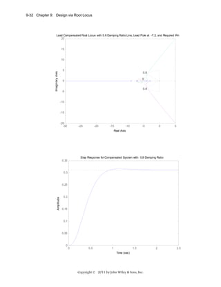
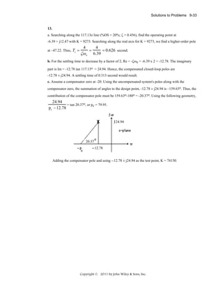
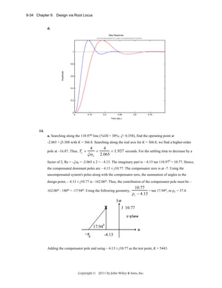
![Solutions to Problems 9-35
b. Searching the real axis segments for K = 5443 yields higher-order poles at approximately –8.12 and
–42.02. The pole at –42.02 can be neglected since it is more than five times further from the
imaginary axis than the dominant pair. The pole at –8.12 may not be canceling the zero at -7. Hence,
simulate to be sure the requirements are met.
c.
Program:
'Uncompensated System G1(s)'
numg1=1;
deng1=poly([-15 (-3+2*j) (-3-2*j)]);
G1=tf(numg1,deng1)
G1zpk=zpk(G1)
K1=366.8
'T1(s)'
T1=feedback(K1*G1,1);
T1zpk=zpk(T1)
'Compensator Gc(s)'
numc=[1 7];
denc=[1 37.4];
Gc=tf(numc,denc)
'Compensated System G2(s) = G1(s)Gc(s)'
K2=5443
G2=G1*Gc;
G2zpk=zpk(G2)
'T2(s)'
T2=feedback(K2*G2,1);
T2zpk=zpk(T2)
step(T1,T2)
title(['Uncompensated and Lead Compensated Systems'])
Computer response:
ans =
Uncompensated System G1(s)
Transfer function:
1
-------------------------s^3 + 21 s^2 + 103 s + 195
Zero/pole/gain:
1
----------------------(s+15) (s^2 + 6s + 13)
K1 =
366.8000
ans =
T1(s)
Zero/pole/gain:
366.8
--------------------------------(s+16.87) (s^2 + 4.132s + 33.31)
Copyright © 2011 by John Wiley & Sons, Inc.](https://image.slidesharecdn.com/solutionscontrolsystemsengineeringbynormannice6ed-130502172814-phpapp02-131105052456-phpapp01/85/Solutions-control-system-sengineering-by-normannice-6ed-130502172814-phpapp02-522-320.jpg)
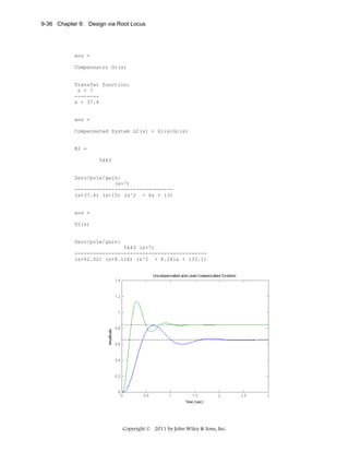
![Solutions to Problems 9-37
15.
a. Searching the 15% overshoot line (121.127o) for 180o yields -0.372 + j0.615. Hence, Ts =
4
=
σd
4
0.372 = 10.75 seconds.
4
4
b. For 7 seconds settling time, σd = T = 7 = 0.571. ωd = 0.571 tan (180o - 121.127o) = 0.946.
s
Therefore, the design point is -0.571 + j0.946. Summing the angles of the uncompensated system's
poles as well as the compensator pole at -15 yields -213.493o. Therefore, the compensator zero must
contribute (213.493o - 180o) = 33.493o. Using the geometry below,
jω
s-plane
j0.946
33.493o
-zc
σ
-0.571
0.946
o
zc - 0.571 = tan (33.493 ) . Hence, zc = 2. The compensated open-loop transfer function is
K(s+2)
. Evaluating the gain for this function at the point, -0.571 + j0.946 yields K
s(s+1)(s2+10s+26)(s+15)
= 207.512.
c.
Program:
numg= 207.512*[1 2];
r=roots([1,10,26]);
deng=poly([0 ,-1, r(1),r(2),-15]);
'G(s)'
G=tf(numg,deng);
Gzpk=zpk(G)
T=feedback(G,1);
step(T)
title(['Step Response for Design of Ts = 7, %OS = 15'])
Computer response:
ans =
G(s)
Zero/pole/gain:
207.512 (s+2)
------------------------------s (s+15) (s+1) (s^2 + 10s + 26)
Copyright © 2011 by John Wiley & Sons, Inc.](https://image.slidesharecdn.com/solutionscontrolsystemsengineeringbynormannice6ed-130502172814-phpapp02-131105052456-phpapp01/85/Solutions-control-system-sengineering-by-normannice-6ed-130502172814-phpapp02-524-320.jpg)
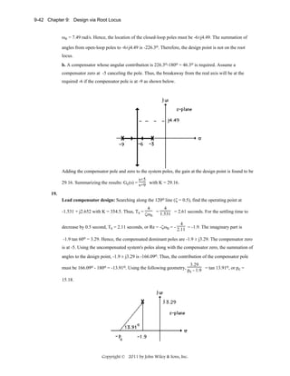
![Solutions to Problems 9-43
Adding the compensator pole and using -1.9 ± j3.29 as the test point, K = 1417.
Computer simulations yield the following: Uncompensated: Ts = 3 seconds, %OS = 14.6%.
Compensated: Ts = 2.3 seconds, %OS = 15.3%.
Lag compensator design: The lead compensated open-loop transfer function is
GLC(s) =
1417(s + 5)
. The uncompensated
(s + 2)(s + 4)(s + 6)(s + 8)(s + 15.18)
1
Kp = 354.5/(2 x 4 x 6 x 8) = 0.923. Hence, the uncompensated steady-state error is 1+K
p
= 0.52.
Since we want 30 times improvement, the lag-lead compensated system must have a steady-state
error of 0.52/30 = 0.017. The lead compensated Kp = 1417*5/(2*4*6*8*15.18) = 1.215. Hence, the
1
lead-compensated error is 1+K = 0.451. Thus, the lag compensator must improve the leadp
1
compensated error by 0.451/0.017 = 26.529 times. Thus 0.451/ ( 1+K
pllc
) = 26.529, where Kpllc =
57.823 is the lead-lag compensated system's position constant. Thus, the improvement in Kp from the
lead to the lag-lead compensated system is 57.823/1.215 = 47.59. Use a lag compensator, whose zero
is 47.59 times farther than its pole, or Glag =
loop transfer function is GLLC(s) =
(s + 0.04759)
. Thus, the lead-lag compensated open(s + 0.001)
1417(s + 5)(s + 0.04759)
.
(s + 2)(s + 4)(s + 6)(s + 8)(s + 15.18)(s + 0.001)
20.
Program:
numg=1;
deng=poly([-2 -4 -6 -8]);
'G(s)'
G=tf(numg,deng);
Gzpk=zpk(G)
rlocus(G,0:5:500)
z=0.5;
pos=exp(-pi*z/sqrt(1-z^2))*100;
sgrid(z,0)
title(['Uncompensated Root Locus with ' , num2str(z), ' Damping Ratio
Line'])
[K,p]=rlocfind(G); %Allows input by selecting point on graphic
'Closed-loop poles = '
p
i=input('Give pole number that is operating point
');
'Summary of estimated specifications for uncompensated system'
operatingpoint=p(i)
gain=K
estimated_settling_time=4/abs(real(p(i)))
estimated_peak_time=pi/abs(imag(p(i)))
estimated_percent_overshoot=pos
estimated_damping_ratio=z
estimated_natural_frequency=sqrt(real(p(i))^2+imag(p(i))^2)
Kpo=dcgain(K*G)
T=feedback(K*G,1);
Copyright © 2011 by John Wiley & Sons, Inc.](https://image.slidesharecdn.com/solutionscontrolsystemsengineeringbynormannice6ed-130502172814-phpapp02-131105052456-phpapp01/85/Solutions-control-system-sengineering-by-normannice-6ed-130502172814-phpapp02-530-320.jpg)
![9-44 Chapter 9: Design via Root Locus
'Press any key to continue and obtain the step response'
pause
step(T)
whitebg('w')
title(['Step Response for Uncompensated System with ' , num2str(z),...
' Damping Ratio'],'color','black')
'Press any key to go to Lead compensation'
pause
'Compensated system'
b=5;
'Lead Zero at -b '
done=1;
while done>0
a=input('Enter a Test Lead Compensator Pole, (s+a). a =
');
numgglead=[1 b];
dengglead=conv([1 a],poly([-2 -4 -6 -8]));
'G(s)Glead(s)'
GGlead=tf(numgglead,dengglead);
GGleadzpk=zpk(GGlead)
wn=4/((estimated_settling_time-0.5)*z);
clf
rlocus(GGlead,0:10:2000)
sgrid(z,wn)
axis([-10 0 -5 5])
title(['Lead Compensated Root Locus with ' , num2str(z),...
' Damping Ratio Line, Lead Pole at ', num2str(-a), ', and Required Wn'])
done=input('Are you done? (y=0,n=1) ');
end
[K,p]=rlocfind(GGlead); %Allows input by selecting point on graphic
'Closed-loop poles = '
p
i=input('Give pole number that is operating point
');
'Summary of estimated specifications for lead-compensated system'
operatingpoint=p(i)
gain=K
estimated_settling_time=4/abs(real(p(i)))
estimated_peak_time=pi/abs(imag(p(i)))
estimated_percent_overshoot=pos
estimated_damping_ratio=z
estimated_natural_frequency=sqrt(real(p(i))^2+imag(p(i))^2)
Kplead=dcgain(K*GGlead)
T=feedback(K*GGlead,1);
'Press any key to continue and obtain the step response'
pause
step(T)
whitebg('w')
title(['Step Response for Lead Compensated System with ' , num2str(z),...
' Damping Ratio'],'color','black')
'Press any key to continue and design lag compensation'
pause
'Improvement in steady-state error with lead compensator is'
error_improvement=(1+Kplead)/(1+Kpo)
additional_error_improvement=30/error_improvement
Kpnn=additional_error_improvement*(1+Kplead)-1
pc=0.001
zc=pc*(Kpnn/Kplead)
numggleadlag=conv(numgglead,[1 zc]);
denggleadlag=conv(dengglead,[1 pc]);
'G(s)Glead(s)Glag(s)'
GGleadGlag=tf(numggleadlag,denggleadlag);
GGleadGlagzpk=zpk(GGleadGlag)
Copyright © 2011 by John Wiley & Sons, Inc.](https://image.slidesharecdn.com/solutionscontrolsystemsengineeringbynormannice6ed-130502172814-phpapp02-131105052456-phpapp01/85/Solutions-control-system-sengineering-by-normannice-6ed-130502172814-phpapp02-531-320.jpg)
![Solutions to Problems 9-45
rlocus(GGleadGlag,0:10:2000)
z=0.5;
pos=exp(-pi*z/sqrt(1-z^2))*100;
sgrid(z,0)
title(['Lag-Lead Compensated Root Locus with ' , num2str(z), ...
' Damping Ratio Line and Lag Pole at ',num2str(-pc)])
[K,p]=rlocfind(GGleadGlag); %Allows input by selecting point on graphic
'Closed-loop poles = '
p
i=input('Give pole number that is operating point
');
'Summary of estimated specifications for lag-lead compensated system'
operatingpoint=p(i)
gain=K
estimated_settling_time=4/abs(real(p(i)))
estimated_peak_time=pi/abs(imag(p(i)))
estimated_percent_overshoot=pos
estimated_damping_ratio=z
estimated_natural_frequency=sqrt(real(p(i))^2+imag(p(i))^2)
Kpleadlag=dcgain(K*GGleadGlag)
T=feedback(K*GGleadGlag,1);
'Press any key to continue and obtain the step response'
pause
step(T)
whitebg('w')
title(['Step Response for Lag-Lead Compensated System with ',
num2str(z),...
' Damping Ratio and Lag Pole at ',num2str(-pc)],'color','black')
Computer response:
ans =
G(s)
Zero/pole/gain:
1
----------------------(s+8) (s+6) (s+4) (s+2)
Select a point in the graphics window
selected_point =
-1.5036 + 2.6553i
ans =
Closed-loop poles =
Copyright © 2011 by John Wiley & Sons, Inc.](https://image.slidesharecdn.com/solutionscontrolsystemsengineeringbynormannice6ed-130502172814-phpapp02-131105052456-phpapp01/85/Solutions-control-system-sengineering-by-normannice-6ed-130502172814-phpapp02-532-320.jpg)
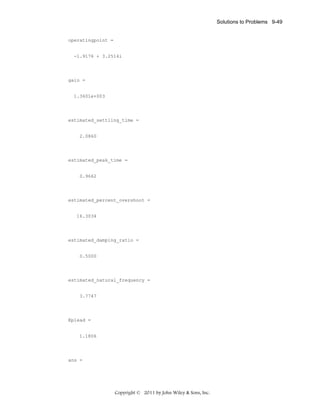
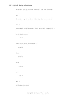
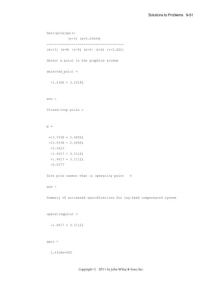
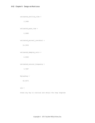
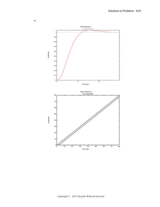
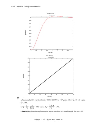
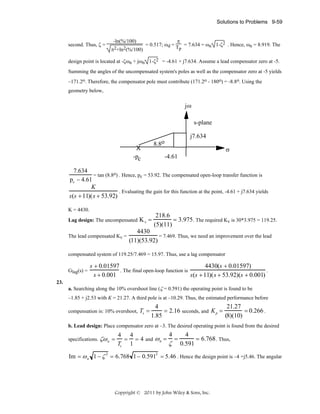
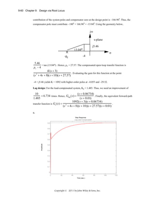
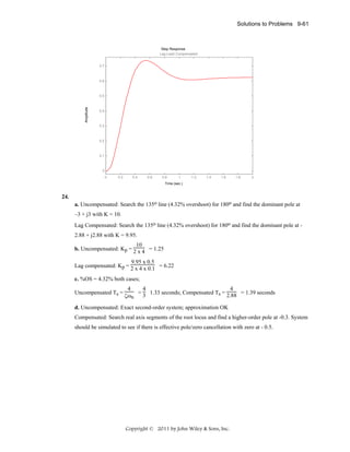
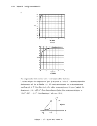
![9-64 Chapter 9: Design via Root Locus
26.
a. The desired operating point is found from the desired specifications. ζω n =
ωn =
2
ζ
=
4 4
= = 2 and
Ts 2
2
= 4.954 . Thus, Im = ωn 1 − ζ 2 = 4.954 1 − 0.40372 = 4.5324 . Hence
0.4037
the design point is –2 +j4.5324. Now, add a pole at the origin to increase system type and drive error
to zero for step inputs.
Now design a PD controller. The angular contribution to the design point of the system poles and pole
at the origin is 101.90. Thus, the compensator zero must contribute 1800 – 101.90 =78.10. Using the
geometry below,
4.5324
= tan(78.10 ) . Hence, zc = 2.955. The compensated open-loop transfer function with PD
zc − 2
compensation is
K ( s + 2.955)
. Adding the compensator zero to the system and
s( s + 4)(s + 6)(s + 10)
evaluating the gain for this at the point –2 + j4.5324 yields K = 294.51 with a higher-order pole at
-2.66 and -13.34.
PI design: Use
Ge ( s) =
GPI (s) =
(s + 0.01)
. Hence, the equivalent open-loop transfer function is
s
K ( s + 2.955)( s + 0.01)
with K = 294.75.
s 2 ( s + 4)( s + 6)( s + 10)
b.
Program (Step Response):
numg=[-2.995 -0.01];
deng=[0 0 -4 -6 -10];
K=294.75;
G=zpk(numg,deng,K)
T=feedback(G,1);
step(T)
Computer response:
Zero/pole/gain:
Copyright © 2011 by John Wiley & Sons, Inc.](https://image.slidesharecdn.com/solutionscontrolsystemsengineeringbynormannice6ed-130502172814-phpapp02-131105052456-phpapp01/85/Solutions-control-system-sengineering-by-normannice-6ed-130502172814-phpapp02-551-320.jpg)
![Solutions to Problems 9-65
294.75 (s+2.995) (s+0.01)
------------------------s^2 (s+4) (s+6) (s+10)
Program (Ramp Response):
numg=[-2.995 -0.01];
deng=[0 0 -4 -6 -10];
K=294.75;
G=zpk(numg,deng,K)
T=feedback(G,1);
Ta=tf([1],[1 0]);
step(T*Ta)
Computer response:
Zero/pole/gain:
294.75 (s+2.995) (s+0.01)
------------------------s^2 (s+4) (s+6) (s+10)
Copyright © 2011 by John Wiley & Sons, Inc.](https://image.slidesharecdn.com/solutionscontrolsystemsengineeringbynormannice6ed-130502172814-phpapp02-131105052456-phpapp01/85/Solutions-control-system-sengineering-by-normannice-6ed-130502172814-phpapp02-552-320.jpg)
![9-66 Chapter 9: Design via Root Locus
27.
Program:
numg=[]
deng=[-4 -6 -10]
'G(s)'
G=zpk(numg,deng,1)
pos=input('Type desired percent overshoot ');
z=-log(pos/100)/sqrt(pi^2+[log(pos/100)]^2);
Ts=input('Type desired settling time ');
zci=input(...
'Type desired position of integral controller zero (absolute value) ');
wn=4/(Ts*z);
desired_pole=(-z*wn)+(wn*sqrt(1-z^2)*i)
angle_at_desired_pole=(180/pi)*angle(evalfr(G,desired_pole))
PD_angle=180-angle_at_desired_pole;
zcpd=((imag(desired_pole)/tan(PD_angle*pi/180))-real(desired_pole));
'PD Compensator'
numcpd=[1 zcpd];
dencpd=[0 1];
'Gcpd(s)'
Gcpd=tf(numcpd,dencpd)
Gcpi=zpk([-zci],[0],1)
Ge=G*Gcpd*Gcpi
rlocus(Ge)
sgrid(z,0)
title(['PID Compensated Root Locus with ' ,...
num2str(pos), '% Damping Ratio Line'])
[K,p]=rlocfind(Ge);
'Closed-loop poles = '
p
f=input('Give pole number that is operating point
');
'Summary of estimated specifications for selected point'
'on PID compensated root locus'
operatingpoint=p(f)
gain=K
Copyright © 2011 by John Wiley & Sons, Inc.](https://image.slidesharecdn.com/solutionscontrolsystemsengineeringbynormannice6ed-130502172814-phpapp02-131105052456-phpapp01/85/Solutions-control-system-sengineering-by-normannice-6ed-130502172814-phpapp02-553-320.jpg)
![Solutions to Problems 9-67
estimated_settling_time=4/abs(real(p(f)))
estimated_peak_time=pi/abs(imag(p(f)))
estimated_percent_overshoot=pos
estimated_damping_ratio=z
estimated_natural_frequency=sqrt(real(p(f))^2+imag(p(f))^2)
T=feedback(K*Ge,1);
step(T)
title(['Step Response for PID Compensated System with ' ,...
num2str(pos),'% Damping Ratio Line'])
pause
one_over_s=tf(1,[1 0]);
Tr=T*one_over_s;
t=0:0.01:10;
step(one_over_s,Tr)
title('Ramp Response for PID Compensated System')
Computer response:
numg =
[]
deng =
0
-4
-6
-10
ans =
G(s)
Zero/pole/gain:
1
-------------------s (s+4) (s+6) (s+10)
Type desired percent overshoot 25
Type desired settling time 2
Type desired position of integral controller zero (absolute value) 0.01
desired_pole =
-2.0000 + 4.5324i
angle_at_desired_pole =
101.8963
ans =
PD Compensator
ans =
Copyright © 2011 by John Wiley & Sons, Inc.](https://image.slidesharecdn.com/solutionscontrolsystemsengineeringbynormannice6ed-130502172814-phpapp02-131105052456-phpapp01/85/Solutions-control-system-sengineering-by-normannice-6ed-130502172814-phpapp02-554-320.jpg)
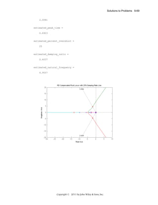
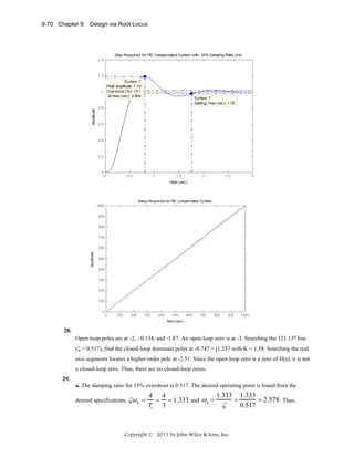
![Solutions to Problems 9-71
Im = ω n 1 − ζ = 2.578 1− 0.517 = 2.207 . Hence the design point is –1.333 + j2.207. The
2
2
angular contribution of the system poles and compensator zero at the design point is 100.80. Thus, the
compensator zero must contribute 1800 – 100.80 = 79.20. Using the geometry below,
jω
s-plane
j2.207
X
-zc
79.2o
-1.333
σ
2.207
= tan (79.2o) . Hence, zc = 1.754. The compensated open-loop transfer function with PD
zc − 1.333
compensation is
K ( s + 1.754)
. Evaluating the gain for this function at the point
s(s + 2)(s + 4)( s + 6)
–1.333 + j2.207 yields K = 47.28 with higher-order poles at –1.617 and –7.718. Following
Figure 9.49(c) in the text,
1
= 1.754 . Therefore, K f = 0.5701 . Also, using the notation of
Kf
Figure 9.49(c), K1 K f = 47.28 , from which K1 = 82.93 .
b.
Program:
K1=82.93;
numg=K1;
deng=poly([0 -2 -4 -6]);
'G(s)'
G=tf(numg,deng);
Gzpk=zpk(G)
Kf=0.5701
numh=Kf*[1 1.754];
denh=1
'H(s)'
H=tf(numh,denh);
Hzpk=zpk(H)
'T(s)'
T=feedback(G,H);
T=minreal(T)
step(T)
title('Step Response for Feedback Compensated System')
Computer response:
ans =
G(s)
Copyright © 2011 by John Wiley & Sons, Inc.](https://image.slidesharecdn.com/solutionscontrolsystemsengineeringbynormannice6ed-130502172814-phpapp02-131105052456-phpapp01/85/Solutions-control-system-sengineering-by-normannice-6ed-130502172814-phpapp02-558-320.jpg)
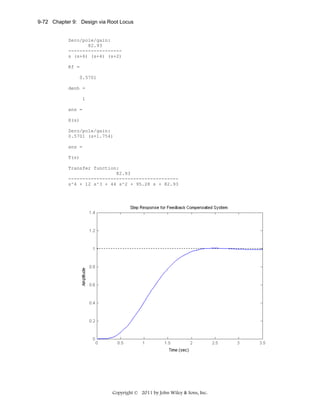
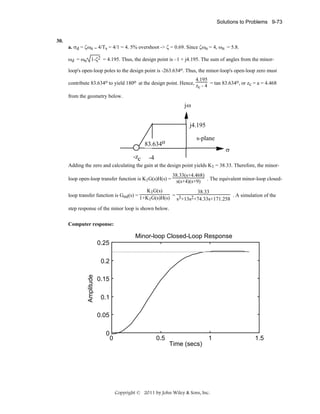
![9-74 Chapter 9: Design via Root Locus
b. The major-loop open-loop transfer function is
G e (s) =
38.33K
.
s + 13s + 74.33s + 171.258
3
2
Drawing the root locus using Ge(s) and searching along the 10% overshoot line (ζ = 0.591) for 180o
yields the point -3.349 + j4.572 with a gain 38.33K = 31.131, or K = 0.812.
c.
Program:
numg=31.131;
deng=[1 13 74.33 171.258];
'G(s)'
G=tf(numg,deng)
T=feedback(G,1);
step(T)
title('Major-loop Closed-Loop Response')
Computer response:
G(s)
Transfer function:
31.13
-----------------------------s^3 + 13 s^2 + 74.33 s + 171.3
d. Adding the PI compensator, Ge(s) =
31.131(s+0.1)
.
s(s3+13s2+74.33s+171.258)
Copyright © 2011 by John Wiley & Sons, Inc.](https://image.slidesharecdn.com/solutionscontrolsystemsengineeringbynormannice6ed-130502172814-phpapp02-131105052456-phpapp01/85/Solutions-control-system-sengineering-by-normannice-6ed-130502172814-phpapp02-561-320.jpg)
![Solutions to Problems 9-75
Program:
numge=31.131*[1 0.1];
denge=[1 13 74.33 171.258 0];
'Ge(s)'
Ge=tf(numge,denge)
T=feedback(Ge,1);
t=0:0.1:10;
step(T,t)
title('Major-loop Closed-Loop Response with PI Compensator')
pause
step(T)
title('Major-loop Closed-Loop Response with PI Compensator')
Computer response:
ans =
Ge(s)
Transfer function:
31.13 s + 3.113
---------------------------------s^4 + 13 s^3 + 74.33 s^2 + 171.3 s
Copyright © 2011 by John Wiley & Sons, Inc.](https://image.slidesharecdn.com/solutionscontrolsystemsengineeringbynormannice6ed-130502172814-phpapp02-131105052456-phpapp01/85/Solutions-control-system-sengineering-by-normannice-6ed-130502172814-phpapp02-562-320.jpg)

![Solutions to Problems 9-81
0.04*[1/0.0001 1]
1
s
Constant
Simulation with GC ( s ) =
Gc(s)
n(s)
d(s)
G(s)
0.04(1 + s / 0.0001)
s
Copyright © 2011 by John Wiley & Sons, Inc.
Scope](https://image.slidesharecdn.com/solutionscontrolsystemsengineeringbynormannice6ed-130502172814-phpapp02-131105052456-phpapp01/85/Solutions-control-system-sengineering-by-normannice-6ed-130502172814-phpapp02-568-320.jpg)
![9-96 Chapter 9: Design via Root Locus
d.
Program:
numg= 1897.125*[1 0.1988];
deng=poly([0 -40 -9.431 -.001]);
'G(s)'
G=tf(numg,deng);
Gzpk=zpk(G)
rlocus(G)
pos=10
z=-log(pos/100)/sqrt(pi^2+[log(pos/100)]^2)
sgrid(z,0)
title(['Root Locus with ' , num2str(pos), ' Percent Overshoot Line'])
[K,p]=rlocfind(G) %Allows input by selecting point on graphic
pause
T=feedback(K*G,1);
step(T)
title(['Step Response for Design of ' , num2str(pos), ' Percent'])
Computer response:
ans =
G(s)
Zero/pole/gain:
1897.125 (s+0.1988)
---------------------------s (s+40) (s+9.431) (s+0.001)
pos =
10
z =
0.5912
Select a point in the graphics window
selected_point =
-3.3649 + 4.8447i
K =
0.9090
Copyright © 2011 by John Wiley & Sons, Inc.](https://image.slidesharecdn.com/solutionscontrolsystemsengineeringbynormannice6ed-130502172814-phpapp02-131105052456-phpapp01/85/Solutions-control-system-sengineering-by-normannice-6ed-130502172814-phpapp02-583-320.jpg)
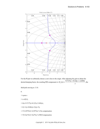
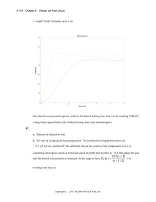
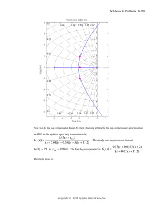
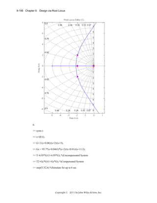
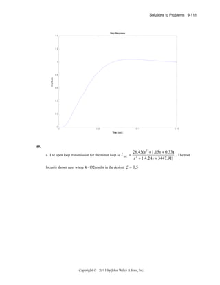
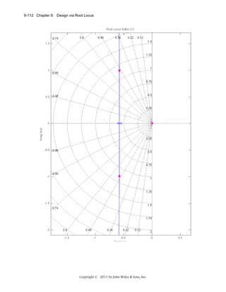

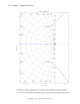

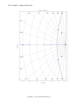
![9-124 Chapter 9: Design via Root Locus
b. The required ess = 0.075 , which corresponds to a K p =
procedure of Section 9.2, let
1 − ess
= 12.33 . Following the
ess
zc K pN
12.33
=
=
= 2.2 . Arbitrarily let pc = 0.01 , so
pc K po 5.7234
zc = 0.022 . The resulting compensator is Gc ( s ) =
3( s + 0.022)
( s + 0.01)
c. We decided to use SIMULINK for this simulation. The block diagram is given by:
9078 *[1/0.43
1
3
/9.6 1 ],[1/0.5
Constant
Gain
Transfer Fcn
Scope
1
3
s+0.022
9078 *[1/0.43
s+0.01
Constant 1
Gain 1
/9.6 1 ],[1/0.5
Transfer Fcn 2
Transfer Fcn 1
The resulting simulation shows the improvement in steady state error without affecting much the
transient response.
54.
1. As can be seen from the entries in the first column of Table P9.54 below, we need to improve the
steady-state error of this system as well as its transient response.
Copyright © 2011 by John Wiley & Sons, Inc.](https://image.slidesharecdn.com/solutionscontrolsystemsengineeringbynormannice6ed-130502172814-phpapp02-131105052456-phpapp01/85/Solutions-control-system-sengineering-by-normannice-6ed-130502172814-phpapp02-611-320.jpg)
![Solutions to Problems 9-127
3.
The following MATLAB M-file was written to simulate the system and plot its step response (shown below) to
check whether all requirements may be met using a PD controller.
numg = 125*[1 1225 2.53E6];
deng = [1 1225 503E4 625E5];
Gp = tf(numg, deng);
%Gp is the transfer function (TF) of the plant
numh = 200;
denh = [1 200];
H = tf(numh, denh);
%H is the TF of the feedback low-pass filter
Zc = 433.9;
numgc = [1 Zc];
dengc = 1;
Gc = tf(numgc, dengc);
%Gc is the TF of the PD Controller
rlocus(Gp*Gc*H);
axis ([-250, 0, -250, 250]);
z=0.707;
sgrid(z,0)
title('Root Locus Zoomed-in around Dominant Poles with a 0.707 Damping Line')
[K1,p]=rlocfind(Gp*Gc*H);
pause
K = K1;
T=feedback((K*Gc*Gp),H);
%T is the closed-loop TF of the system
step(750*T);
axis ([0, 0.04, 0, 1300]);
grid
title(['Step Response of PD-cont. Bus Voltage for Zc = - ', num2str(Zc)]);
Copyright © 2011 by John Wiley & Sons, Inc.](https://image.slidesharecdn.com/solutionscontrolsystemsengineeringbynormannice6ed-130502172814-phpapp02-131105052456-phpapp01/85/Solutions-control-system-sengineering-by-normannice-6ed-130502172814-phpapp02-614-320.jpg)
![9-130 Chapter 9: Design via Root Locus
Gc(s)G p(s)H(s) =
25000 K (s 2 + 1225 s + 2.53 ×10 6 )(s + 800)(s + Z PI )
.
s(s 3 + 1225 s 2 + 503 × 10 4 s + 625 ×10 5 )(s + 200)
The following MATLAB M-file was written to add the integral mode. It was run a few times with various values of
the PI controller’s zero, ZPI, (between zero and the closest open-loop pole at -12.5) to check whether all
requirements are met using a PID controller.
numg = 125*[1 1225 2.53E6];
deng = [1 1225 503E4 625E5];
Gp = tf(numg, deng);
%Gp is the transfer function (TF) of the plant
numh = 200;
denh = [1 200];
H = tf(numh, denh);
%H is the TF of the feedback low-pass filter
Zc = 800;
Zi = 4;
numgc = poly ([-Zi, -Zc]);
dengc = [1 0];
Gc = tf(numgc, dengc);
%Gc is the TF of the PID Controller
rlocus(Gp*Gc*H);
axis ([-200, 0, -200, 200]);
z=0.707;
sgrid (z,0)
title('Root Locus Zoomed-in around Dominant Poles with a 0.707 Damping Line')
[K1,p]=rlocfind(Gp*Gc*H);
pause
K = K1;
T=feedback((K*Gc*Gp),H);
%T is the closed-loop TF of the system
step(750*T);
Copyright © 2011 by John Wiley & Sons, Inc.](https://image.slidesharecdn.com/solutionscontrolsystemsengineeringbynormannice6ed-130502172814-phpapp02-131105052456-phpapp01/85/Solutions-control-system-sengineering-by-normannice-6ed-130502172814-phpapp02-617-320.jpg)
![Solutions to Problems 9-131
axis ([0, 0.4, 0, 850]);
grid
title(['Step Response of PID-cont. of DC Bus for Zc = -',num2str(Zc),' and Zi
= - ',num2str(Zi),]);
PID Root Locus Zoomed-in around Dominant Poles with a 0.707 Damping Line
200
0.707
150
System: PID-Cont
Gain: 0.00298
Pole: -125 + 125i
Damping: 0.707
Overshoot (%): 4.33
Frequency (rad/sec): 177
100
Imaginary Axis
50
0
-50
-100
-150
0.707
-200
-200
-180
-160
-140
-120
-100
-80
-60
-40
-20
0
Real Axis
6.
As a result, the following transfer function of the PID controller was found:
⎛
⎛ s 2 + 804 s + 3200 ⎞
⎟=
Gc( s ) = 0.003 × ⎜
⎜
⎟
s
⎝
⎠
K3 ⎜ s 2 +
⎜
⎜
⎝
K1
K ⎞
s+ 2 ⎟
⎟
K3
K3 ⎟
⎠
.
s
Thus, the gains, K1, K2, and K3 are: K3 = 0.003; K1 = 2.41; and K2 = 9.6.
7.
The system simulation showed that all steady-state and transient response requirements have been met (see the
figure below and Table P9.54).
Copyright © 2011 by John Wiley & Sons, Inc.](https://image.slidesharecdn.com/solutionscontrolsystemsengineeringbynormannice6ed-130502172814-phpapp02-131105052456-phpapp01/85/Solutions-control-system-sengineering-by-normannice-6ed-130502172814-phpapp02-618-320.jpg)
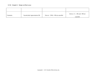

![9-136 Chapter 9: Design via Root Locus
From which, zc = 24.09. Putting this into the forward path,
0.6488K (s+53.85)(s2 + 16s + 9200)(s+24.09)
Get(s) =
(s2 + 8.119s + 376.3) (s^2 + 15.47s + 9283)(s+60)2
Using root locus, the gain 0.6488K = 1637, or K = 2523.
b. Add a PI controller
GPI (s) =
(s + 0.1)
s
Thus,
0.6488K (s+53.85)(s2 + 16s + 9200)(s+24.09)(s+0.1)
Get(s) =
s (s2 + 8.119s + 376.3) (s^2 + 15.47s + 9283)(s+60)2
_____
Using root locus, the gain 0.6488K = 1740, or K = 2682.
c.
Program:
syms s
numg=1637*(s+53.85)*(s^2+16*s+9200)*(s+24.09)*(s+0.1);
deng=s*(s^2+15.47*s+9283)*(s^2+8.119*s+376.3)*(s+60)^2;
numg=sym2poly(numg);
deng=sym2poly(deng);
G=tf(numg,deng);
Gzpk=zpk(G)
T=feedback(G,1);
step(T,0:0.01:1)
title(['With PD, Notch, and PI'])
pause
step(T)
title(['With PD, Notch, and PI'])
Computer response:
Zero/pole/gain:
Copyright © 2011 by John Wiley & Sons, Inc.](https://image.slidesharecdn.com/solutionscontrolsystemsengineeringbynormannice6ed-130502172814-phpapp02-131105052456-phpapp01/85/Solutions-control-system-sengineering-by-normannice-6ed-130502172814-phpapp02-623-320.jpg)
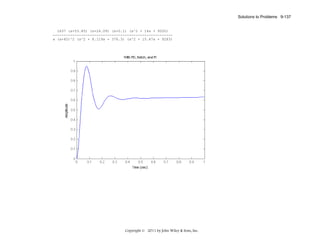
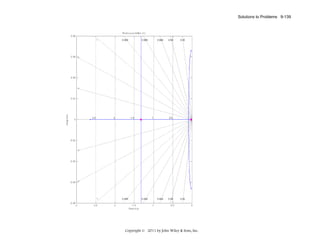

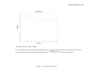
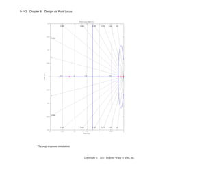

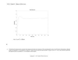
![Solutions to Problems 9-145
numg = [1 0.6];
deng = poly ([-0.0163 -0.5858]);
G = tf(numg, deng);
rlocus(G);
axis ([-0.8, 0.1, -0.1, 0.1]);
pos=(0);
z=-log(pos/100)/sqrt(pi^2+(log(pos/100))^2);
sgrid(z,0)
title(['Root Locus with ', num2str(pos) , ' Percent Overshoot Line'])
[K1,p]=rlocfind(G);
pause
T=feedback(K1*G,1);
%Tu is the closed-loop TF of the uncompensated system
T=minreal(T);
step(4*T);
xlabel ('Time')
ylabel ('Speed Sensor Output, c(t) in volts')
title (['Step Response of Uncompensated System at K = ', num2str(K1), ' to a 4 volt Input Step'])
grid
Copyright © 2011 by John Wiley & Sons, Inc.](https://image.slidesharecdn.com/solutionscontrolsystemsengineeringbynormannice6ed-130502172814-phpapp02-131105052456-phpapp01/85/Solutions-control-system-sengineering-by-normannice-6ed-130502172814-phpapp02-632-320.jpg)
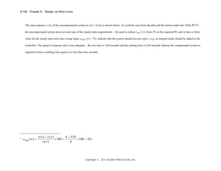
![9-148 Chapter 9: Design via Root Locus
Thus, we obtain a type-1 system with a transfer function1 of the “Plant & Compensator” given by: G ( s ) =
constant
K1 ( s + 0.6)
, which has a “position” error
s ( s + 0.5858)
K P = lim G ( s) = ∞ and a “velocity” error constant, K v = lim sG ( s) = 1.024 K1 .
s →0
s →0
Hence, the requirement to have a zero steady-state error for a step input, r(t) = A u(t) = 4 u(t) is satisfied, since: estep (∞ ) =
A
4
=
=0.
1+ K P 1+ ∞
1
1
=
≤ 0.02 , e.g., if K1 ≥ 48.83 . At this value of
K v 1.024 K1
48.83 s + 29.3
K1, the open-loop transfer function of the PI-compensated system is: G ( s ) =
.
s ( s + 0.5858)
The requirement that eramp(∞) ≤ 2%, for a unit-ramp input will be satisfied if eramp (∞ ) =
The following MATLAB file was written to check whether all requirements have been met:
numg = [48.83 29.3];
deng = poly ([0 -0.5858]);
G = tf(numg, deng);
T = feedback(G,1);
%T is the closed-loop TF of the PI_compensated system
T = minreal(T);
step(4*T);
1
Enter this transfer function and the results obtained for the PI-compensated system into Table P9.57.
Copyright © 2011 by John Wiley & Sons, Inc.](https://image.slidesharecdn.com/solutionscontrolsystemsengineeringbynormannice6ed-130502172814-phpapp02-131105052456-phpapp01/85/Solutions-control-system-sengineering-by-normannice-6ed-130502172814-phpapp02-635-320.jpg)
![Solutions to Problems 9-149
axis ([0, 0.2, 0, 5]);
grid
xlabel ('Time')
ylabel ('Speed Sensor Output, c(t) in volts')
title ('PI-compensated Systems Response to a 4 volt Input Step')
pause
numr = 1;
denr = poly (0);
R = tf(numr, denr);
T2 = R*T;
E= R-T2;
%E = Ramp error of PI_compensated system
step(T2,'b', R,'g', E,'r');
axis ([0, 5, 0, 5]);
grid
xlabel ('Time')
ylabel ('Output Rate, dc(t)/dt, V/s (Blue); Unit Ramp (Green); Error (Red)');
title ('Response of PI-compensated System to a Unit-ramp Input')
Copyright © 2011 by John Wiley & Sons, Inc.](https://image.slidesharecdn.com/solutionscontrolsystemsengineeringbynormannice6ed-130502172814-phpapp02-131105052456-phpapp01/85/Solutions-control-system-sengineering-by-normannice-6ed-130502172814-phpapp02-636-320.jpg)
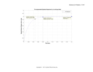
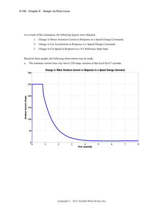
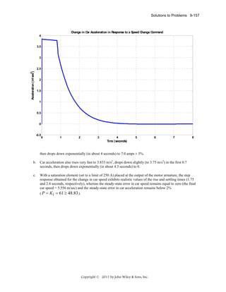
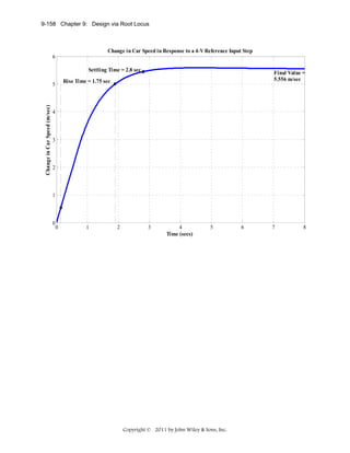
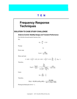
![10-2 Chapter 10: Frequency Response Methods
a. Phase is 180o at ω = 11.5 rad/s. At this frequency the gain is - 48.41 dB, or K = 263.36. Therefore,
for stability, 0 < K < 263.36.
b. If K = 3, the magnitude curve will be 9.54 dB higher and go through zero dB at ω = 0.94 rad/s. At
this frequency, the phase response is -125.99o. Thus, the phase margin is 180o - 125.99o = 54.01o.
Using Eq. (10.73), ζ = 0.528. Eq. (4.38) yields %OS = 14.18%.
c.
Program:
numga=50.88;
denga=poly([0 -1.32 -100]);
'Ga(s)'
Ga=tf(numga,denga);
Gazpk=zpk(Ga)
'(a)'
bode(Ga)
title('Bode Plot at Gain of 50.88')
pause
[Gm,Pm,Wcp,Wcg]=margin(Ga);
'Gain for Stability'
Gm
pause
'(b)'
numgb=50.88*3;
dengb=denga;
'Gb(s)'
Gb=tf(numgb,dengb);
Gbzpk=zpk(Gb)
bode(Gb)
title('Bode Plot at Gain of 3*50.88')
[Gm,Pm,Wcp,Wcg]=margin(Gb);
'Phase Margin'
Pm
for z=0:.01:1
Pme=atan(2*z/(sqrt(-2*z^2+sqrt(1+4*z^4))))*(180/pi);
if Pm-Pme<=0;
break
end
end
z
percent=exp(-z*pi/sqrt(1-z^2))*100
Computer response:
ans =
Copyright © 2011 by John Wiley & Sons, Inc.](https://image.slidesharecdn.com/solutionscontrolsystemsengineeringbynormannice6ed-130502172814-phpapp02-131105052456-phpapp01/85/Solutions-control-system-sengineering-by-normannice-6ed-130502172814-phpapp02-647-320.jpg)
![Answers to Review Questions 10-5
3. Separate magnitude and phase curves; polar plot
4. If the transfer function of the system is G(s), let s=jω. The resulting complex number's magnitude is the
magnitude response, while the resulting complex number's angle is the phase response.
5. Bode plots are asymptotic approximations to the frequency response displayed as separate magnitude and
phase plots, where the magnitude and frequency are plotted in dB.
6. Negative 6 dB/octave which is the same as 20 dB/decade
7. Negative 24 dB/octave or 80 dB/decade
8. Negative 12 dB/octave or 40 dB/decade
9. Zero degrees until 0.2; a negative slope of 45o/decade from a frequency of 0.2 until 20; a constant -90o
phase from a frequency of 20 until ∞
10. Second-order systems require a correction near the natural frequency due to the peaking of the curve for
different values of damping ratio. Without the correction the accuracy is in question.
11. Each pole yields a maximum difference of 3.01 dB at the break frequency. Thus for a pole of
multiplicity three, the difference would be 3x3.01 or 9.03 dB at the break frequency, - 4.
12. Z = P - N, where Z = # of closed-loop poles in the right-half plane, P = # of open-loop poles in the righthalf plane, and N = # of counter-clockwise encirclements of -1 made by the mapping.
13. Whether a system is stable or not since the Nyquist criterion tells us how many rhp the system has
14. A Nyquist diagram, typically, is a mapping, through a function, of a semicircle that encloses the right
half plane.
15. Part of the Nyquist diagram is a polar frequency response plot since the mapping includes the positive jω
axis.
16. The contour must bypass them with a small semicircle.
17. We need only map the positive imaginary axis and then determine that the gain is less than unity when
the phase angle is 180o.
18. We need only map the positive imaginary axis and then determine that the gain is greater than unity
when the phase angle is 180o.
19. The amount of additional open-loop gain, expressed in dB and measured at 180o of phase shift, required
to make a closed-loop system unstable.
20. The phase margin is the amount of additional open-loop phase shift, ΦM, required at unity gain to make
the closed-loop system unstable.
21. Transient response can be obtained from (1) the closed-loop frequency response peak, (2) phase margin
22. a. Find T(jω)=G(jω)/[1+G(jω)H(jω)] and plot in polar form or separate magnitude and phase plots. b.
Superimpose G(jω)H(jω) over the M and N circles and plot. c. Superimpose G(jω)H(jω) over the Nichols
chart and plot.
Copyright © 2011 by John Wiley & Sons, Inc.](https://image.slidesharecdn.com/solutionscontrolsystemsengineeringbynormannice6ed-130502172814-phpapp02-131105052456-phpapp01/85/Solutions-control-system-sengineering-by-normannice-6ed-130502172814-phpapp02-650-320.jpg)
![10-12 Chapter 10: Frequency Response Methods
7.
Gain dB
0
-50
-100
-150 -1
10
10 0
101
102
101
102
Frequency (rad/sec)
Phase deg
0
-90
-180
-270
10-1
10 0
Frequency (rad/sec)
8.
Program:
numg=[1 5];
deng=conv([1 6 100],[1 4 25]);
G=tf(numg,deng);
'G(s)'
Gzpk=zpk(G)
nyquist(G)
axis([-3e-3,4e-3,-5e-3,5e-3])
w=0:0.1:100;
[re,im]=nyquist(G,w);
for i=1:1:length(w)
M(i)=abs(re(i)+j*im(i));
A(i)=atan2(im(i),re(i))*(180/pi);
if 180-abs(A(i))<=1;
re(i);
im(i);
K=1/abs(re(i));
fprintf('nw = %g',w(i))
fprintf(', Re = %g',re(i))
fprintf(', Im = %g',im(i))
fprintf(', M = %g',M(i))
fprintf(', Angle = %g',A(i))
fprintf(', K = %g',K)
Gm=20*log10(1/M(i));
fprintf(', Gm = %g',Gm)
break
end
end
Computer response:
ans =
G(s)
Zero/pole/gain:
(s+5)
Copyright © 2011 by John Wiley & Sons, Inc.](https://image.slidesharecdn.com/solutionscontrolsystemsengineeringbynormannice6ed-130502172814-phpapp02-131105052456-phpapp01/85/Solutions-control-system-sengineering-by-normannice-6ed-130502172814-phpapp02-657-320.jpg)
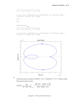
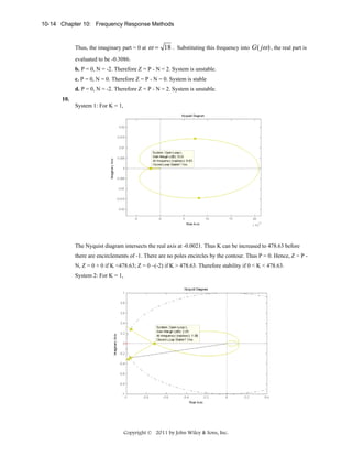
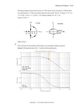
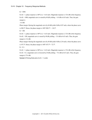
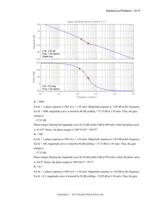
![Solutions to Problems 10-19
K = 0.1:
For K = 1, phase response is 180o at ω = 1.41 rad/s. Magnitude response is 0 dB at this frequency.
For K = 0.1, magnitude curve is lowered by 20 dB yielding -20 dB at 1.41 rad/s. Thus, the gain
margin is 20 dB.
Phase margin: Lowering the magnitude curve by 20 dB yields no frequency where the magnitude
curve is 0 dB. Hence, the phase margin is infinite.
12.
Program:
%Enter G(s)************************
numg=1;
deng=poly([0 -3 -12]);
'G(s)'
G=tf(numg,deng)
w=0.01:0.1:100;
%Enter K **************************
K=input('Type gain, K ');
bode(K*G,w)
pause
[M,P]=bode(K*G,w);
%Calculate Gain Margin**************
for i=1:1:length(P);
if P(i)<=-180;
fprintf('nGain K = %g',K)
fprintf(', Frequency(180 deg) = %g',w(i))
fprintf(', Magnitude = %g',M(i))
fprintf(', Magnitude (dB) = %g',20*log10(M(i)))
fprintf(', Phase = %g',P(i))
Gm=20*log10(1/M(i));
fprintf(', Gain Margin (dB) = %g',Gm)
break
end
end
%Calculate Phase Margin**************
for i=1:1:length(M);
if M(i)<=1;
fprintf('nGain K = %g',K)
fprintf(', Frequency (0 dB) = %g',w(i))
fprintf(', Magnitude = %g',M(i))
fprintf(', Magnitude (dB) = %g',20*log10(M(i)))
fprintf(', Phase = %g',P(i))
Pm=180+P(i);;
fprintf(', Phase Margin = %g',Pm)
break
end
end
'Alternate program using MATLAB margin function:'
clear
clf
%Bode Plot and Find Points
%Enter G(s)************************
numg=1;
deng=poly([0 -3 -12]);
'G(s)'
G=tf(numg,deng)
w=0.01:0.1:100;
Copyright © 2011 by John Wiley & Sons, Inc.](https://image.slidesharecdn.com/solutionscontrolsystemsengineeringbynormannice6ed-130502172814-phpapp02-131105052456-phpapp01/85/Solutions-control-system-sengineering-by-normannice-6ed-130502172814-phpapp02-664-320.jpg)
![10-20 Chapter 10: Frequency Response Methods
%Enter K **************************
K=input('Type gain, K ');
bode(K*G,w)
[Gm,Pm,Wcp,Wcg]=margin(K*G)
'Gm(dB)'
20*log10(Gm)
Computer response:
ans =
G(s)
Transfer function:
1
------------------s^3 + 15 s^2 + 36 s
Type gain, K 40
Gain K = 40, Frequency(180 deg) = 6.01, Magnitude = 0.0738277, Magnitude
(dB) = -22.6356, Phase = -180.076, Gain Margin (dB) = 22.6356
Gain K = 40, Frequency (0 dB) = 1.11, Magnitude = 0.93481, Magnitude (dB) =
-0.585534, Phase = -115.589, Phase Margin = 64.4107
Copyright © 2011 by John Wiley & Sons, Inc.](https://image.slidesharecdn.com/solutionscontrolsystemsengineeringbynormannice6ed-130502172814-phpapp02-131105052456-phpapp01/85/Solutions-control-system-sengineering-by-normannice-6ed-130502172814-phpapp02-665-320.jpg)

![10-22 Chapter 10: Frequency Response Methods
13.
Program:
numg=8000;
deng=poly([-6 -20 -35]);
G=tf(numg,deng)
ltiview
Computer response:
Transfer function:
8000
---------------------------s^3 + 61 s^2 + 1030 s + 4200
Copyright © 2011 by John Wiley & Sons, Inc.](https://image.slidesharecdn.com/solutionscontrolsystemsengineeringbynormannice6ed-130502172814-phpapp02-131105052456-phpapp01/85/Solutions-control-system-sengineering-by-normannice-6ed-130502172814-phpapp02-667-320.jpg)
![10-24 Chapter 10: Frequency Response Methods
14.
⎛ 1 ⎞
yields
Squaring Eq. (10.51) and setting it equal to
⎝ 2⎠
2
ωn4
(ωn2 - ω2)2 + 4ζ2ωn2ω2
1
=2
Simplifying,
ω 4 + 2ωn2(2ζ2 - 1)ω2 - ωn4 = 0
Solving for ω2 using the quadratic formula and simplifying yields,
ω2 = ωn2 [ - (2ζ2 - 1) ±
4ζ4 - 4ζ2 + 2 ]
Taking the square root and selecting the positive term,
ω = ωn
15.
(1 - 2ζ2) +
4ζ4 - 4ζ2 + 2
a. Using Eq. (10.55), ωBW = 10.06 rad/s.
Copyright © 2011 by John Wiley & Sons, Inc.](https://image.slidesharecdn.com/solutionscontrolsystemsengineeringbynormannice6ed-130502172814-phpapp02-131105052456-phpapp01/85/Solutions-control-system-sengineering-by-normannice-6ed-130502172814-phpapp02-669-320.jpg)
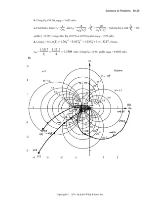
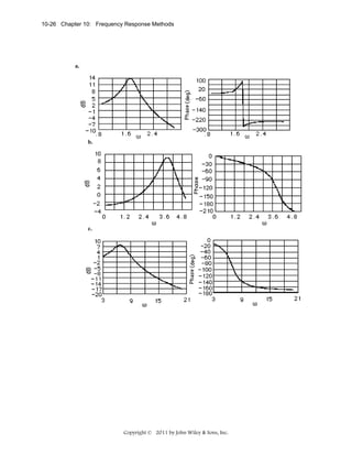
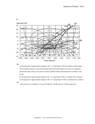
![10-28 Chapter 10: Frequency Response Methods
(a)
v=0.3
(c)
0.5
v=1
0.8
-355
o
1.0
-5
o
2
(b)
v=2
o
-340
o
-10
3
1.4
o
-20
5
-320
4
o
7
5
3
6
10
o
o
-60
-300
-280
o
-40
o
o
o
o
o
-200
-270 -260
-240
-220
o
-180 o-160
o
o
-140
o
-120
-100
o
o
-90
o
-80
Systems (a) and (b) are both unstable since the open-loop magnitude is greater than unity when the
open-loop phase is 180o. System (c) is tangent to approximately M = 3. Using Figure 10.40, we
estimate 58% overshoot.
20.
Program:
%Enter G(s)***********************
numg=[1 5];
deng=[1 4 25 0];
'G(s)'
G=tf(numg,deng)
%Enter K *************************
K=input('Type gain, K ');
'T(s)'
T=feedback(K*G,1)
bode(T)
title('Closed-loop Frequency Response')
[M,P,w]=bode(T);
[Mp i]=max(M);
Mp
MpdB=20*log10(Mp)
wp=w(i)
for i=1:1:length(M);
if M(i)<=0.707;
fprintf('Bandwidth = %g',w(i))
break
end
end
Copyright © 2011 by John Wiley & Sons, Inc.](https://image.slidesharecdn.com/solutionscontrolsystemsengineeringbynormannice6ed-130502172814-phpapp02-131105052456-phpapp01/85/Solutions-control-system-sengineering-by-normannice-6ed-130502172814-phpapp02-673-320.jpg)
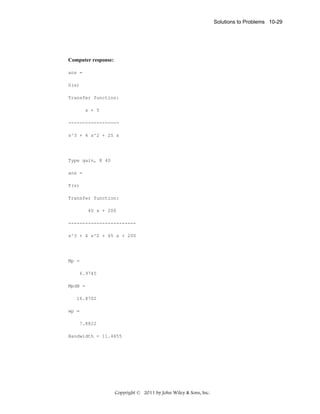
![10-30 Chapter 10: Frequency Response Methods
21.
Program:
numg=[5 30];
deng=[1 4 15 0];
G=tf(numg,deng)
bode(G)
%Make a Bode plot.
title('Open-Loop Frequency Response')
%Add a title to the Bode plot.
[Gm,Pm,Wcp,Wcg]=margin(G);
%Find margins and margin
%frequencies.
'Gain margin(dB); Phase margin(deg.); 0 dB freq. (r/s);'
'180 deg. freq. (r/s)'
%Display label.
margins=[20*log10(Gm),Pm,Wcg,Wcp]
%Display margin data.
ltiview
Computer response:
Transfer function:
5 s + 30
-----------------s^3 + 4 s^2 + 15 s
ans =
Gain margin(dB); Phase margin(deg.); 0 dB freq. (r/s);
Copyright © 2011 by John Wiley & Sons, Inc.](https://image.slidesharecdn.com/solutionscontrolsystemsengineeringbynormannice6ed-130502172814-phpapp02-131105052456-phpapp01/85/Solutions-control-system-sengineering-by-normannice-6ed-130502172814-phpapp02-675-320.jpg)
![Solutions to Problems 10-31
ans =
180 deg. freq. (r/s)
margins =
15.5649
65.1103
2.4319
6.7088
22.
Program:
%Enter G(s)************************************
numg=5*[1 6];
deng=[1 4 15 0];
'Open-Loop System'
'G(s)'
G=tf(numg,deng)
clf
w=.10:1:10;
nichols(G,w)
ngrid
title('Nichols Plot')
Copyright © 2011 by John Wiley & Sons, Inc.](https://image.slidesharecdn.com/solutionscontrolsystemsengineeringbynormannice6ed-130502172814-phpapp02-131105052456-phpapp01/85/Solutions-control-system-sengineering-by-normannice-6ed-130502172814-phpapp02-676-320.jpg)
![10-32 Chapter 10: Frequency Response Methods
[M,P]=nichols(G,w);
for i=1:1:length(M);
if M(i)<=0.45;
BW=w(i);
break
end
end
pause
MpdB=input('Enter Mp in dB from Nichols Plot ');
Mp=10^(MpdB/20);
z2=roots([4,-4,(1/Mp^2)]);%Since Mp=1/sqrt(4z^2(1-z^2))
z1=sqrt(z2);
z=min(z1);
Pos=exp(-z*pi/(sqrt(1-z^2)));
Ts=(4/(BW*z))*sqrt((1-z^2)+sqrt(4*z^4-4*z^2+2));
Tp=(pi/(BW*sqrt(1-z^2)))*sqrt((1-z^2)+sqrt(4*z^4-4*z^2+2));
'Closed-Loop System'
'T(s)'
T=feedback(G,1)
bode(T)
title('Closed-Loop Frequency Response Plots')
fprintf('nDamping Ratio = %g',z)
fprintf(', Percent Overshoot = %g',Pos*100)
fprintf(', Bandwidth = %g',BW)
fprintf(', Mp (dB) = %g',MpdB)
fprintf(', Mp = %g',Mp)
fprintf(', Settling Time = %g',Ts)
fprintf(', Peak Time = %g',Tp)
pause
step(T)
title('Closed-Loop Step Response')
Computer response:
ans =
Open-Loop System
ans =
G(s)
Transfer function:
5 s + 30
-----------------s^3 + 4 s^2 + 15 s
Enter Mp in dB from Nichols Plot
0
ans =
Closed-Loop System
ans =
T(s)
Transfer function:
Copyright © 2011 by John Wiley & Sons, Inc.](https://image.slidesharecdn.com/solutionscontrolsystemsengineeringbynormannice6ed-130502172814-phpapp02-131105052456-phpapp01/85/Solutions-control-system-sengineering-by-normannice-6ed-130502172814-phpapp02-677-320.jpg)
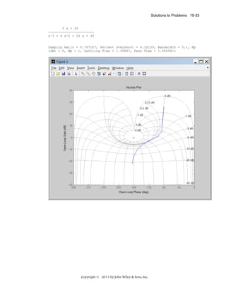
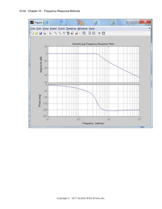
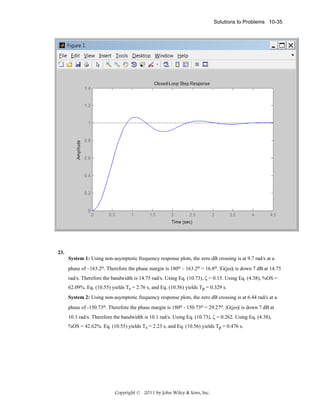
![10-36 Chapter 10: Frequency Response Methods
24.
a.
Gain dB
50
0
-50 -1
10
10
1
10 2
10
10 0
1
10
Frequency (rad/sec)
Phase deg
-60
-90
-120
-150
-180
10
-1
10
0
2
Frequency (rad/sec)
b. Zero dB frequency = 7.8023; Looking at the phase diagram at this frequency, the phase margin is
8.777 degrees. Using Eq. (10.73) or Figure 10.48, ζ = 0.08. Thus, %OS = 77.7.
c.
Step Response for K = 40
1.6
1.4
1.2
Amplitude
1
0.8
0.6
0.4
0.2
0
0
1
2
3
4
5
6
Time (secs)
7
8
9
10
25.
From the Bode plots: Gain margin = 14.96 dB; phase margin = 49.570; 0 dB frequency = 2.152 rad/s;
1800 frequency = 6.325 rad/s; bandwidth(@-7 dB point) = 3.8 rad/s. From Eq. (10.73) ζ = 0.48; from
Eq. (4.38) %OS = 17.93; from Eq. (10.55) Ts = 2.84 s; from Eq. (10.56) Tp = 1.22 s.
26.
Program:
G=zpk([-2],[0 -1 -4],100)
%G=zpk([-3 -5],[0 -2 -4 -6],50)
G=tf(G)
Copyright © 2011 by John Wiley & Sons, Inc.](https://image.slidesharecdn.com/solutionscontrolsystemsengineeringbynormannice6ed-130502172814-phpapp02-131105052456-phpapp01/85/Solutions-control-system-sengineering-by-normannice-6ed-130502172814-phpapp02-681-320.jpg)
![Solutions to Problems 10-37
bode(G)
title('System 1')
%title('System 2')
pause
%Find Phase Margin
[Gm,Pm,Wcg,Wcp]=margin(G);
w=1:.01:20;
[M,P,w]=bode(G,w);
%Find Bandwidth
for k=1:1:length(M);
if 20*log10(M(k))+7<=0;
'Mag'
20*log10(M(k))
'BW'
wBW=w(k)
break
end
end
%Find Damping Ratio,Percent Overshoot, Settling Time, and Peak Time
for z= 0:.01:10
Pt=atan(2*z/(sqrt(-2*z^2+sqrt(1+4*z^4))))*(180/pi);
if (Pm-Pt)<=0
z;
Po=exp(-z*pi/sqrt(1-z^2));
Ts=(4/(wBW*z))*sqrt((1-2*z^2)+sqrt(4*z^4-4*z^2+2));
Tp=(pi/(wBW*sqrt(1-z^2)))*sqrt((1-2*z^2)+sqrt(4*z^4-4*z^2+2));
fprintf('Bandwidth = %g ',wBW)
fprintf('Phase Margin = %g',Pm)
fprintf(', Damping Ratio = %g',z)
fprintf(', Percent Overshoot = %g',Po*100)
fprintf(',Settling Time = %g',Ts)
fprintf(', Peak Time = %g',Tp)
break
end
end
T=feedback(G,1);
step(T)
title('Step Response System 1')
%title('Step Response System 2')
Computer response:
Zero/pole/gain:
100 (s+2)
------------s (s+1) (s+4)
Transfer function:
100 s + 200
----------------s^3 + 5 s^2 + 4 s
ans =
Mag
ans =
-7.0007
Copyright © 2011 by John Wiley & Sons, Inc.](https://image.slidesharecdn.com/solutionscontrolsystemsengineeringbynormannice6ed-130502172814-phpapp02-131105052456-phpapp01/85/Solutions-control-system-sengineering-by-normannice-6ed-130502172814-phpapp02-682-320.jpg)
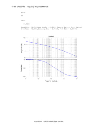
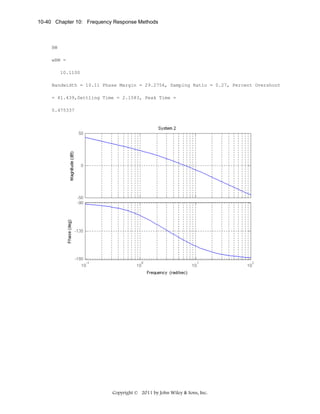
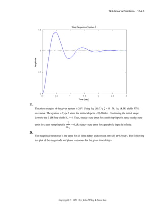
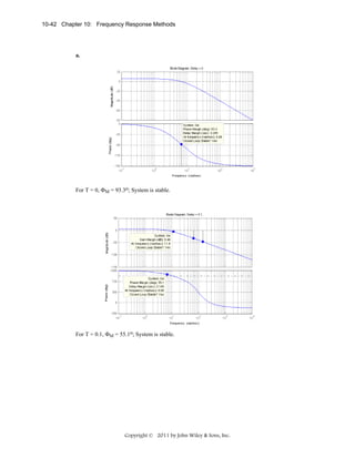
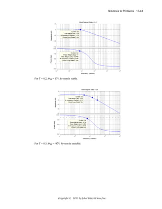
![Solutions to Problems 10-45
Gain dB
0
-50
-100
-150 -1
10
10 0
10 1
10 2
Frequency (rad/sec)
Phase deg
0
-360
-720
-1080
-1440
-1
10
10
0
10
1
10
2
Frequency (rad/sec)
The phase is -180o at 2.12 rad/s. At this frequency, the gain is -34.76 dB. Thus the gain can be raised
by 34.76 dB = 54.71. Hence for stability, 0<K<54.71.
30.
The Bode plots for K = 40 and a delay of 0.5 second is shown below.
Gain dB
50
0
-50
-100 -1
10
10 0
10 1
10 2
Frequency (rad/sec)
0
Phase deg
-360
-720
-1080
-1440
-1
10
10
0
10
1
10
2
Frequency (rad/sec)
The magnitude curve crosses zero dB at a frequency of 1.0447 rad/s. At this frequency, the phase plot
shows a phase margin of 35.74 degrees. Using Eq. (10.73) or Figure 10.48, ζ = 0.33. Thus, %OS =
33.3.
31.
Program:
%Enter G(s)************************
numg1=1;
deng1=poly([0 -3 -12]);
'G1(s)'
G1=tf(numg1,deng1)
[numg2,deng2]=pade(0.5,5);
Copyright © 2011 by John Wiley & Sons, Inc.](https://image.slidesharecdn.com/solutionscontrolsystemsengineeringbynormannice6ed-130502172814-phpapp02-131105052456-phpapp01/85/Solutions-control-system-sengineering-by-normannice-6ed-130502172814-phpapp02-690-320.jpg)
![10-46 Chapter 10: Frequency Response Methods
'G2(s) (delay)'
G2=tf(numg2,deng2)
'G(s)=G1(s)G2(s)'
G=G1*G2
%Enter K **************************
K=input('Type gain, K ');
T=feedback(K*G,1);
step(T)
title(['Step Response for K = ',num2str(K)])
Computer response:
ans =
G1(s)
Transfer function:
1
------------------s^3 + 15 s^2 + 36 s
ans =
G2(s) (delay)
Transfer function:
-s^5 + 60 s^4 - 1680 s^3 + 2.688e004 s^2 - 2.419e005 s + 9.677e005
-----------------------------------------------------------------s^5 + 60 s^4 + 1680 s^3 + 2.688e004 s^2 + 2.419e005 s + 9.677e005
ans =
G(s)=G1(s)G2(s)
Transfer function:
-s^5 + 60 s^4 - 1680 s^3 + 2.688e004 s^2 - 2.419e005 s + 9.677e005
-------------------------------------------------------------------------s^8 + 75 s^7 + 2616 s^6 + 5.424e004 s^5 + 7.056e005 s^4 + 5.564e006 s^3
+ 2.322e007 s^2 + 3.484e007 s
Copyright © 2011 by John Wiley & Sons, Inc.](https://image.slidesharecdn.com/solutionscontrolsystemsengineeringbynormannice6ed-130502172814-phpapp02-131105052456-phpapp01/85/Solutions-control-system-sengineering-by-normannice-6ed-130502172814-phpapp02-691-320.jpg)
![10-48 Chapter 10: Frequency Response Methods
Original-1/s Magnitude
30
Magnitude (dB)
25
20
15
10
5
0
-5
10 -1
10 0
10 1
10 2
10 1
10 2
Frequency (rad/s)
Original-1/s
0
Phase (deg)
-20
-40
-60
-80
-100
10 -1
10 0
Frequency (rad/s)
Original-1/s(s+5.3) Magnitude
60
40
20
0
-20
10 -1
10 0
10 1
10 2
10 1
10 2
Frequency (rad/s)
Original-1/s(s+5.3)
8
6
4
2
0
-2
-4
10 -1
10 0
Frequency (rad/s)
Estimated K = 41 dB = 112. Therefore, final estimate is
G(s) =
112
.
s(s + 5.3)
33.
Program:
%Generate total system Bode plots - numg0,deng0 - M0,P0
clf
numg0=12*poly([-1 -20]);
deng0=conv([1 7],[1 4 100]);
G0=tf(numg0,deng0);
w=0.1:0.1:100;
Copyright © 2011 by John Wiley & Sons, Inc.](https://image.slidesharecdn.com/solutionscontrolsystemsengineeringbynormannice6ed-130502172814-phpapp02-131105052456-phpapp01/85/Solutions-control-system-sengineering-by-normannice-6ed-130502172814-phpapp02-693-320.jpg)
![Solutions to Problems 10-49
[M0,P0]=bode(G0,w);
M0=M0(:,:);
P0=P0(:,:);
[20*log10(M0),P0,w];
bode(G0,w)
pause
%Subtract (s+1) [numg1,deng1] and generate Bode plot-M2,P2
numg1=[1 1];
deng1=1;
G1=tf(numg1,deng1);
[M1,P1]=bode(G1,w);
M1=M1(:,:);
P1=P1(:,:);
M2=20*log10(M0)-20*log10(M1);
P2=P0-P1;
clf
subplot(2,1,1)
semilogx(w,M2)
grid
subplot(2,1,2)
semilogx(w,P2)
grid
pause
%Subtract10^2/(s^2+2*0.3*10s+10^2) [numg2,deng2] and generate Bode plotM4,P4
numg2=100;
deng2=[1 2*0.3*10 10^2];
G2=tf(numg2,deng2);
[M3,P3]=bode(G2,w);
M3=M3(:,:);
P3=P3(:,:);
M4=M2-20*log10(M3);
P4=P2-P3;
clf
subplot(2,1,1)
semilogx(w,M4)
grid
subplot(2,1,2)
semilogx(w,P4)
grid
pause
%Subtract(8.5/23)(s+23)/(s+8.5) [numg3,deng3] and generate Bode plot-M6,P6
numg3=(8.5/23)*[1 23];
deng3=[1 8.5];
G3=tf(numg3,deng3);
[M5,P5]=bode(G3,w);
M5=M5(:,:);
P5=P5(:,:);
M6=M4-20*log10(M5);
P6=P4-P5;
clf
subplot(211)
semilogx(w,M6)
grid
subplot(212)
semilogx(w,P6)
grid
Copyright © 2011 by John Wiley & Sons, Inc.](https://image.slidesharecdn.com/solutionscontrolsystemsengineeringbynormannice6ed-130502172814-phpapp02-131105052456-phpapp01/85/Solutions-control-system-sengineering-by-normannice-6ed-130502172814-phpapp02-694-320.jpg)

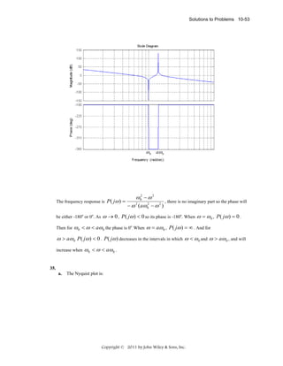
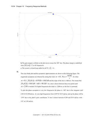
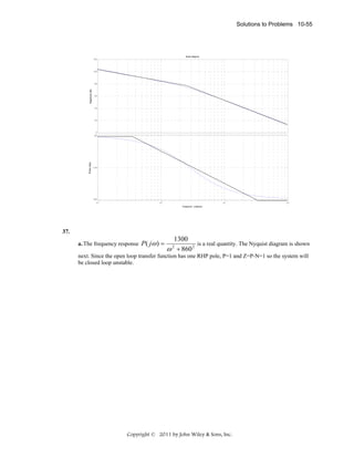
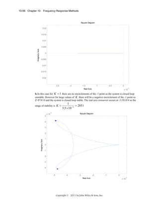
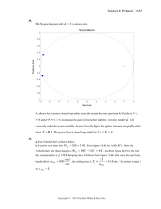
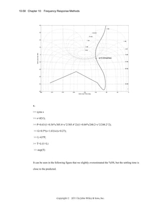
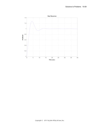
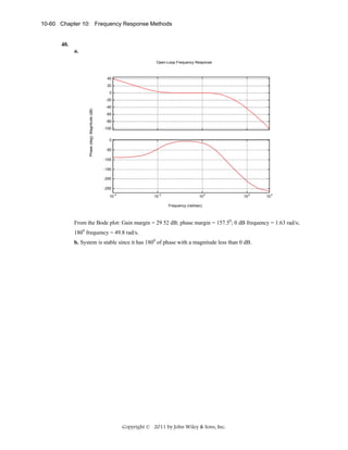
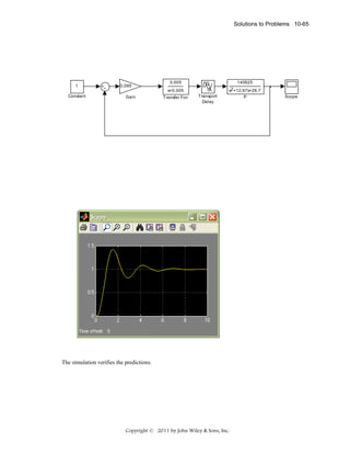
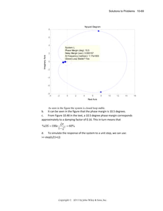
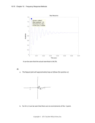
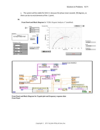
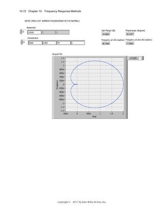
![Solutions to Problems 10-75
The details of the MathScript node code follow:
for zeta=0:0.01:1
newphasemargin=atan(2*zeta/(sqrt(-2*zeta^2+sqrt(1+4*zeta^4))))*(180/pi);
tol=phasemargin-newphasemargin;
if tol<=0
PO=100*exp(-zeta*pi/sqrt(1-zeta^2));
ts=(4/(Bw*zeta))*sqrt((1-2*zeta^2)+sqrt(4*zeta^4-4*zeta^2+2));
tp=(pi/(Bw*sqrt(1-zeta^2)))*sqrt((1-2*zeta^2)+sqrt(4*zeta^4-4*zeta^2+2));
break
end;
end;
52.
The following MATLAB file was used to plot the Bode magnitude and phase plots for that system and
to obtain the response of the system, c(t), at a pure delay of 1 second.
numg1 = conv([4 1], [10 1]);
%numerator of G1 without pure delay
deng0 = conv([25 1],[3.333 1]); %the denominator without pure
integrator
deng1 = conv(deng0, [1 0]);
%add pure integrator to denominator
G1 = tf(numg1, deng1);
%G1 is the open-loop TF without pure
delay
[numd,dend]= pade(1,5);
%5th-order Pade approximation of
pure delay
D = (tf (numd, dend));
G = G1*D;
Bode(G);
grid
pause
T = feedback(G,1);
%C.L. TF of the PD_compensated system
T = minreal(T);
step(T);
grid
xlabel ('Time')
ylabel ('Controlled Level, c(t) in p. u.')
title ('Unit Step Response of Water Level in the Steam generator ')
a. The Bode magnitude and phase plots for this system, obtained using fifth-order Pade approximation
for τ = 1 sec, are shown below with minimum stability margins displayed.
Copyright © 2011 by John Wiley & Sons, Inc.](https://image.slidesharecdn.com/solutionscontrolsystemsengineeringbynormannice6ed-130502172814-phpapp02-131105052456-phpapp01/85/Solutions-control-system-sengineering-by-normannice-6ed-130502172814-phpapp02-720-320.jpg)
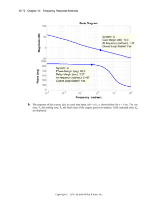
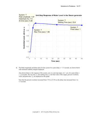
![Solutions to Problems 10-81
55.
a.
The following MATLAB file was used to plot the Bode magnitude and phase plots for that system and
to obtain the response of the system, c(t), to a step input, r(t) = 4 u(t).
K = 0.78;
numg = K*[1 0.6];
deng = poly ([-0.0163 -0.5858]);
G = tf(numg, deng);
bode (G);
grid
pause
T = feedback(G,1);
%T is the closed-loop TF of the P_controlled
system
T = minreal(T);
step(4*T);
grid
Copyright © 2011 by John Wiley & Sons, Inc.](https://image.slidesharecdn.com/solutionscontrolsystemsengineeringbynormannice6ed-130502172814-phpapp02-131105052456-phpapp01/85/Solutions-control-system-sengineering-by-normannice-6ed-130502172814-phpapp02-726-320.jpg)
![Solutions to Problems 10-83
P-controlled System's Response to a 4 volt Input Step
4
System: T
Final Value: 3.92
System: T
Settling Time (sec): 4.69
3.5
Speed Sensor Output, c(t) in volts
System: T
Rise Time (sec): 2.69
3
2.5
2
1.5
1
0.5
0
0
1
2
3
4
5
6
7
Time (sec)
b.
After adding the integral gain to the controller, we substituted the values of K1 = 0.78 and
Zc =
K2
= 0.4 into the transfer function of the plant and compensator. Thus we obtained:
K1
G ( s) =
0.78 × ( s + 0.4) ( s + 0.6)
0.78 s 2 + 0.78 s + 0.1872
.
=
s ( s + 0.5858) ( s + 0.016 3) s ( s + 0.5858) ( s + 0.016 3)
The following MATLAB file was written to plot the Bode magnitude and phase plots for that system
and to obtain the response of the system, c(t), to a step input, r(t) = 4 u(t).
numg = [0.78 0.78 0.1872];
deng = poly ([0 -0.0163 -0.5858]);
G = tf(numg, deng);
bode (G);
grid
pause
T = feedback(G,1);
%T is the closed-loop TF of the PI-controlled
system
T = minreal(T);
step(4*T);
grid
xlabel ('Time')
ylabel ('Speed Sensor Output, c(t) in volts')
title ('PI-controlled Systems Response to a 4 volt Input Step')
The Bode magnitude and phase plots obtained are shown below with the minimum stability margins
displayed on the phase plot.
Copyright © 2011 by John Wiley & Sons, Inc.](https://image.slidesharecdn.com/solutionscontrolsystemsengineeringbynormannice6ed-130502172814-phpapp02-131105052456-phpapp01/85/Solutions-control-system-sengineering-by-normannice-6ed-130502172814-phpapp02-728-320.jpg)

![E L E V E N
Design via
Frequency Response
SOLUTIONS TO CASE STUDIES CHALLENGES
Antenna Control: Gain Design
a. The required phase margin for 25% overshoot (ζ = 0.404), found from Eq. (10.73), is 43.49o.
50.88K
From the solution to the Case Study Challenge problem of Chapter 10, G(s) = s(s+1.32)(s+100) .
Using the Bode plots for K = 1 from the solution to the Case Study Challenge problem of
Chapter 10, we find the required phase margin at ω = 1.35 rad/s, where the magnitude response
is -14 dB. Hence, K = 5.01 (14 dB).
b.
Program:
%Input system
numg=50.88;
deng=poly([0 -1.32 -100]);
G=tf(numg,deng);
%Percent Overshoot to Damping Ratio to Phase Margin
Po=input('Type %OS ');
z=(-log(Po/100))/(sqrt(pi^2+log(Po/100)^2));
Pm=atan(2*z/(sqrt(-2*z^2+sqrt(1+4*z^4))))*(180/pi);
fprintf('nPercent Overshoot = %g',Po)
fprintf(', Damping Ratio = %g',z)
fprintf(', Phase Margin = %g',Pm)
%Get Bode data
bode(G)
pause
w=0.01:0.05:1000;%Step size can be increased if memory low.
[M,P]=bode(G,w);
M=M(:,:);
P=P(:,:);
Ph=-180+Pm;
for i=1:1:length(P);
if P(i)-Ph<=0;
M=M(i);
K=1/M;
fprintf(', Frequency = %g',w(i))
fprintf(', Phase = %g',P(i))
fprintf(', Magnitude = %g',M)
fprintf(', Magnitude (dB) = %g',20*log10(M))
fprintf(', K = %g',K)
break
end
end
T=feedback(K*G,1);
step(T)
Copyright © 2011 by John Wiley & Sons, Inc.](https://image.slidesharecdn.com/solutionscontrolsystemsengineeringbynormannice6ed-130502172814-phpapp02-131105052456-phpapp01/85/Solutions-control-system-sengineering-by-normannice-6ed-130502172814-phpapp02-731-320.jpg)
![Solutions to Case Studies Challenges 11-3
Antenna Control: Cascade Compensation Design
50.88K
a. From the solution to the previous Case Study Challenge in this chapter, G(s) = s(s+1.32)(s+100) .
For Kv = 20, K = 51.89. Hence, the gain compensated system is
2640.16
G(s) = s(s+1.32)(s+100)
Using Eq. (10.73), 15% overshoot (i.e. ζ = 0.517) requires a phase margin of 53.18o. Using the Bode
plots for K = 1 from the solution to the Case Study Challenge problem of Chapter 10, we find the
required phase margin at ω = 0.97 rad/s where the phase is -126.82o.
To speed up the system, we choose the compensated phase margin frequency to be 4.6 * 0.97 = 4.46
rad/s. Choose the lag compensator break a decade below this frequency, or ω = 0.446 rad/s.
At the phase margin frequency, the phase angle is -166.067o, or a phase margin of 13.93o. Using 5o
leeway, we need to add 53.18o - 13.93o + 5o = 44.25o. From Figure 11.8, β = 0.15, or γ =
1
=
β
6.667. Using Eq. (11.15), the lag portion of the compensator is
GLag (s) =
Using Eqs. (11.9) and (11.15), T2 =
(s+0.446)
s+0.446
0.446 = s+0.0669 .
(s+6.667)
1
ωmax
β
= 0.579. From Eq. (11.15), the lead portion of the
compensator is
s+1.727
GLead (s) = s+11.51
The final forward path transfer function is
2640.16(s+0.446)(s+1.727)
G(s)GLag (s)GLead(s) = s(s+1.32)(s+100)(s+0.0669)(s+11.51)
b.
Program:
%Input system *****************************
K=51.89;
numg=50.88*K;
deng=poly([0 -1.32 -100]);
G=tf(numg,deng);
Po=15;
z=(-log(Po/100))/(sqrt(pi^2+log(Po/100)^2));
%Determine required phase margin**************
Pmreq=atan(2*z/(sqrt(-2*z^2+sqrt(1+4*z^4))))*(180/pi)
phreq=Pmreq-(180)%required phase
w=0.1:0.01:10;
[M,P]=bode(G,w);
for i=1:1:length(P);%search for phase angle
if P(i)-phreq<=0;
ph=P(i)
w(i)
break
end
end
wpm=4.6*w(i)
Copyright © 2011 by John Wiley & Sons, Inc.](https://image.slidesharecdn.com/solutionscontrolsystemsengineeringbynormannice6ed-130502172814-phpapp02-131105052456-phpapp01/85/Solutions-control-system-sengineering-by-normannice-6ed-130502172814-phpapp02-733-320.jpg)
![11-4 Chapter 11: Design via Frequency Response
[M,P]=bode(G,wpm);%Find phase at wpm
Pmreqc=Pmreq-(180+P)+5%Find contribution required from compensator+5
beta=(1-sin(Pmreqc*pi/180))/(1+sin(Pmreqc*pi/180))
%Design lag compensator***************
zclag=wpm/10;
pclag=zclag*beta;
Kclag=beta;
%Design lead compensator**********
zclead=wpm*sqrt(beta);
pclead=zclead/beta;
Kclead=1/beta;
%Create compensated forward path*********
numgclag=Kclag*[1 zclag];
dengclag=[1 pclag];
'Gclag(s)'
Gclag=tf(numgclag,dengclag);
Gclagzpk=zpk(Gclag)
numgclead=Kclead*[1 zclead];
dengclead=[1 pclead];
'Gclead(s)'
Gclead=tf(numgclead,dengclead);
Gcleadzpk=zpk(Gclead)
Gc=Gclag*Gclead;
'Ge(s)=G(s)*Gclag(s)*Gclead(s)'
Ge=Gc*G;
Gezpk=zpk(Ge)
%Test lag-lead compensator****************
T=feedback(Ge,1);
bode(Ge)
title('Lag-lead Compensated')
[Gm,Pm,wcp,wcg]=margin(Ge);
'Compensated System Results'
fprintf('nResulting Phase Margin = %g',Pm)
fprintf(', Resulting Phase Margin Frequency = %g',wcg)
pause
step(T)
title('Lag-lead Compensated')
Computer response:
Pmreq =
53.1718
phreq =
-126.8282
ph =
-126.8660
ans =
0.9700
wpm =
4.4620
Pmreqc =
44.2468
beta =
0.1780
ans =
Copyright © 2011 by John Wiley & Sons, Inc.](https://image.slidesharecdn.com/solutionscontrolsystemsengineeringbynormannice6ed-130502172814-phpapp02-131105052456-phpapp01/85/Solutions-control-system-sengineering-by-normannice-6ed-130502172814-phpapp02-734-320.jpg)
![11-10 Chapter 11: Design via Frequency Response
4.
a. Bode plots for K = 1:
Using Eqs. (4.39) and (10.73) a percent overshoot = 15 is equivalent to a ζ = 0.517 and φM = 53.170.
The phase-margin frequency = 2.61 rad/s where the phase is 53.170 – 1800 = -126.830. The
magnitude = -13 dB, or 0.0.2239. Hence K = 1/ 0.2239 = 4.466.
b.
Program:
G=zpk([-20 -25],[0 -6 -9 -14],1)
K=4.466
T=feedback(K*G,1);
step(T)
Computer response:
Zero/pole/gain:
(s+20) (s+25)
-------------------s (s+6) (s+9) (s+14)
K =
4.466
Copyright © 2011 by John Wiley & Sons, Inc.](https://image.slidesharecdn.com/solutionscontrolsystemsengineeringbynormannice6ed-130502172814-phpapp02-131105052456-phpapp01/85/Solutions-control-system-sengineering-by-normannice-6ed-130502172814-phpapp02-740-320.jpg)
![Solutions to Problems 11-13
frequency, the magnitude = 57.55 dB = 754.2. Hence the lag compensator K = 1/754.2 = 0.001326.
Following Steps 3 and 4 of the lag compensator design procedure in Section 11.3,
s + 0.121
Glag(s) = 0.001326 s + 0.0001604
b.
Program:
%Input system
numg=1473*poly([-10 -11]);
deng=poly([0 -3 -6 -9]);
G=tf(numg,deng);
numc=0.001326*[1 0.121];
denc=[1 0.0001604];
Gc=tf(numc,denc);
Ge=G*Gc;
T=feedback(Ge,1);
step(T)
Computer response:
7.
Uncompensated system:
Searching along the 121.1o line (15% overshoot), find the dominant pole at -2.15 ± j3.56 with K =
97.7. Therefore, the uncompensated static error constant is Kvo =
Copyright © 2011 by John Wiley & Sons, Inc.
97.7
70
= 1.396. On the frequency](https://image.slidesharecdn.com/solutionscontrolsystemsengineeringbynormannice6ed-130502172814-phpapp02-131105052456-phpapp01/85/Solutions-control-system-sengineering-by-normannice-6ed-130502172814-phpapp02-743-320.jpg)
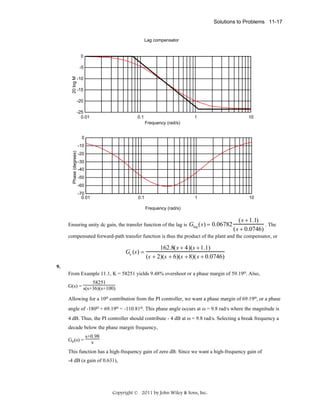
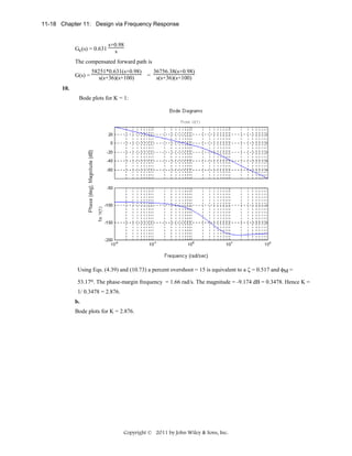
![Solutions to Problems 11-19
Adding 10o to the phase margin yields 63.17. Thus, the required phase is –1800 + 63.170 = -116.830,
which occurs at a frequency of 1.21 rad/s. The magnitude = 3.366 dB = 1.473. Hence, the lag
compensator K = 1/ 1.473 = =0.6787. Selecting the break a decade below the phase-margin
frequency,
Gc(s) = 0.6787
s+0.121
s
c.
Program:
%Input system
numg=2.876*poly([-10 -11]);
deng=poly([0 -3 -6 -9]);
G=tf(numg,deng);
numc=0.6787*[1 0.121];
denc=[1 0];
Gc=tf(numc,denc);
Ge=G*Gc;
T=feedback(Ge,1);
step(T)
Copyright © 2011 by John Wiley & Sons, Inc.](https://image.slidesharecdn.com/solutionscontrolsystemsengineeringbynormannice6ed-130502172814-phpapp02-131105052456-phpapp01/85/Solutions-control-system-sengineering-by-normannice-6ed-130502172814-phpapp02-749-320.jpg)
![11-20 Chapter 11: Design via Frequency Response
Computer response:
11.
Program:
%PI Compensator Design via Frequency Response
%Input system
G=zpk([],[-5 -10],1);
G=tf(G);
%Percent Overshoot to Damping Ratio to Phase Margin
Po=input('Type %OS ');
z=(-log(Po/100))/(sqrt(pi^2+log(Po/100)^2));
Pm=atan(2*z/(sqrt(-2*z^2+sqrt(1+4*z^4))))*(180/pi)+10;
fprintf('nPercent Overshoot = %g',Po)
fprintf(', Damping Ratio = %g',z)
fprintf(', Phase Margin = %g',Pm)
%Get Bode data
bode(G)
title('Uncompensated')
pause
%Find frequency at desired phase margin and the gain at this frequency
w=logspace(-1,2,10000);
%w=.1:0.1:100;
[M,P,w]=bode(G,w);
Ph=-180+Pm
for i=1:1:length(P);
if P(i)-Ph<=0
Mag=M(i)
wf=w(i);
fprintf(', Frequency = %g',wf)
fprintf(', Phase = %g',P(i))
fprintf(', Magnitude = %g',Mag)
fprintf(', Magnitude (dB) = %g',20*log10(Mag))
break
end
end
Copyright © 2011 by John Wiley & Sons, Inc.](https://image.slidesharecdn.com/solutionscontrolsystemsengineeringbynormannice6ed-130502172814-phpapp02-131105052456-phpapp01/85/Solutions-control-system-sengineering-by-normannice-6ed-130502172814-phpapp02-750-320.jpg)
![Solutions to Problems 11-21
%Design PI compensator
%Break frequency is a decade below phase margin frequency
wh=wf/10;
%Magnitude is reciprocal of magnitude of G at the phase margin frequency
%so net magnitude is 0 dB at the phase margin frequency
Kc=1/Mag
'PI Compensator'
Gpi=tf(Kc*[1 wh],[1 0])
bode(Gpi)
title(['PI compensator'])
pause
'G(s)Gpi(s)'
Ge=series(G,Gpi);
Ge=zpk(Ge)
bode(Ge)
title('PI Compensated')
[Gm,Pm,Wcp,Wcg]=margin(Ge);
'Gain margin(dB); Phase margin(deg.); 0 dB freq. (r/s);'
'180 deg. freq. (r/s)'
margins=[20*log10(Gm),Pm,Wcg,Wcp]
pause
T=feedback(Ge,1);
step(T)
title('PI Compensated')
Computer response:
Type %OS
25
Percent Overshoot = 25, Damping Ratio = 0.403713, Phase Margin = 53.463
Ph =
-126.5370
Mag =
0.0037
, Frequency = 14.5518, Phase
(dB) = -48.6811
Kc =
= -126.54, Magnitude = 0.00368082, Magnitude
271.6786
ans =
PI Compensator
Transfer function:
271.7 s + 395.3
--------------s
ans =
G(s)Gpi(s)
Zero/pole/gain:
271.6786 (s+1.455)
-----------------s (s+10) (s+5)
Copyright © 2011 by John Wiley & Sons, Inc.](https://image.slidesharecdn.com/solutionscontrolsystemsengineeringbynormannice6ed-130502172814-phpapp02-131105052456-phpapp01/85/Solutions-control-system-sengineering-by-normannice-6ed-130502172814-phpapp02-751-320.jpg)
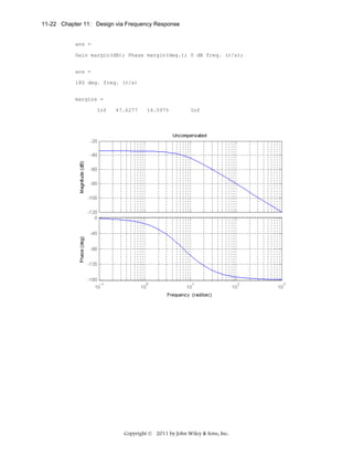
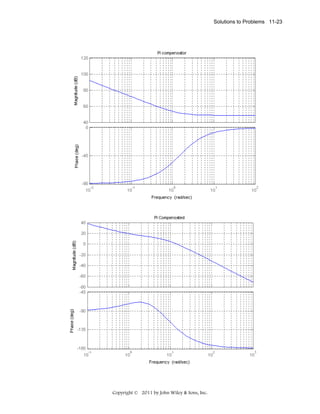
![Solutions to Problems 11-27
Gain dB
50
0
-50
-100 -1
10
100
10 1
Frequency (rad/sec)
10 2
10 3
10 2
10 3
Lead-Compensated System
Phase deg
0
-90
-180
-270
10 -1
100
10 1
Frequency (rad/sec)
Lead-compensated phase margin = 50.2352.
b.
Program:
numg=1000;
deng=poly([0 -5 -20]);
G=tf(numg,deng);
numc=[1 3.51272];
denc=[1 37.7144];
Gc=tf(numc,denc);
Ge=G*10.7366*Gc;
T=feedback(Ge,1);
step(T)
Computer response:
Copyright © 2011 by John Wiley & Sons, Inc.](https://image.slidesharecdn.com/solutionscontrolsystemsengineeringbynormannice6ed-130502172814-phpapp02-131105052456-phpapp01/85/Solutions-control-system-sengineering-by-normannice-6ed-130502172814-phpapp02-757-320.jpg)
![Solutions to Problems 11-31
phase-margin
frequency=j16
80.2
o
-z c
16
1
tan (80.2) = z . Therefore, zc = 2.76. Thus, Gc (s) = 2.76 (s + 2.76) .
c
The PD compensated Bode plots:
Gain dB
50
0
-50 -1
10
10 0
10 1
10 2
10 1
10 2
Frequency (rad/sec)
PD Compensated
Phase deg
-60
-90
-120
-150
-180
10-1
10 0
Frequency (rad/sec)
Compensated phase margin is 62.942o.
b.
Program:
numg=1000;
deng=poly([0 -5 -20]);
G=tf(numg,deng);
numc=(1/2.76)*[1 2.76];
denc=1;
Gc=tf(numc,denc);
Ge=G*Gc;
T=feedback(Ge,1);
step(T)
title('PD Compensated')
Copyright © 2011 by John Wiley & Sons, Inc.](https://image.slidesharecdn.com/solutionscontrolsystemsengineeringbynormannice6ed-130502172814-phpapp02-131105052456-phpapp01/85/Solutions-control-system-sengineering-by-normannice-6ed-130502172814-phpapp02-761-320.jpg)
![11-32 Chapter 11: Design via Frequency Response
Computer response:
17.
Program:
%Lead Compensator Design via Frequency Response
%Input system
K=input('Type K to meet steady-state error ');
numg=K*[1 1];
deng=poly([0 -2 -6]);
'Open-loop system'
'G(s)'
G=tf(numg,deng)
%Generate uncompensated step response
T=feedback(G,1);
step(T)
title('Gain Compensated')
%Input transient response specifications
Po=input('Type %OS ');
%Ts=input('Type settling time
');
Tp=input('Type peak time
');
%Determine required bandwidth
z=(-log(Po/100))/(sqrt(pi^2+log(Po/100)^2));
%wn=4/(z*Ts);
wn=pi/(Tp*sqrt(1-z^2));
wBW=wn*sqrt((1-2*z^2)+sqrt(4*z^4-4*z^2+2));
%Make a Bode plot and get Bode data
%Get Bode data
bode(G)
title('Gain Compensated')
w=0.01:0.1:100;
[M,P]=bode(numg,deng,w);
%Find current phase margin
[Gm,Pm,wcp,wcg]=margin(M,P,w);
%Calculate required phase margin
z=(-log(Po/100))/(sqrt(pi^2+log(Po/100)^2));
Pmreq=atan(2*z/(sqrt(-2*z^2+sqrt(1+4*z^4))))*(180/pi);
Copyright © 2011 by John Wiley & Sons, Inc.](https://image.slidesharecdn.com/solutionscontrolsystemsengineeringbynormannice6ed-130502172814-phpapp02-131105052456-phpapp01/85/Solutions-control-system-sengineering-by-normannice-6ed-130502172814-phpapp02-762-320.jpg)
![Solutions to Problems 11-33
%Add a correction factor of 10 degrees
Pmreqc=Pmreq+10;
%Calculate phase required from compensator
Pc=Pmreqc-Pm;
%Design lead compensator
%Find compensator beta and peak compensator magnitude
beta=(1-sin(Pc*pi/180))/(1+sin(Pc*pi/180));
magpc=1/sqrt(beta);
%Find frequency at which uncompensated system has a magnitude of 1/magpc
%This frequency will be the new phase margin frequency
for i=1:1:length(M);
if M(i)-(1/magpc)<=0;
wmax=w(i);
break
end
end
%Calculate the lead compensator's break frequencies
zc=wmax*sqrt(beta);
pc=zc/beta;
Kc=1/beta;
numc=[1 zc];
denc=[1 pc];
'Gc(s)'
Gc=tf(numc,denc)
%Display data
fprintf('nK = %g',K)
fprintf(' Percent Overshoot = %g',Po)
fprintf(', Damping Ratio = %g',z)
%fprintf(', Settling Time = %g',Ts)
fprintf(', Peak Time = %g',Tp)
fprintf(', Current Phase Margin = %g',Pm)
fprintf(', Required Phase Margin = %g',Pmreq)
fprintf(', Required Phase Margin with Correction Factor = %g',Pmreqc)
fprintf(', Required Bandwidth = %g',wBW)
fprintf(', Required Phase Contribution from Compensator = %g',Pc)
fprintf(', Compensator Beta = %g',beta)
fprintf(', New phase margin frequency = %g',wmax)
fprintf(' Compensator gain, Kc = %g',Kc)
fprintf(' Compensator zero,= %g',-zc)
fprintf(' Compensator pole,= %g',-pc)
'G(s)Gc(s)'
Ge=G*Kc*Gc
pause
%Generate compensated Bode plots
%Make a Bode plot and get Bode data
%Get Bode data
bode(Ge)
title('Lead Compensated')
w=0.01:0.1:1000;
[M,P]=bode(Ge,w);
%Find compensated phase margin
[Gm,Pm,wcp,wcg]=margin(M,P,w);
fprintf('nCompensated Phase Margin,= %g',Pm)
pause
%Generate step response
T=feedback(Ge,1);
step(T)
title('Lead Compensated')
Computer response:
Type K to meet steady-state error
360
ans =
Copyright © 2011 by John Wiley & Sons, Inc.](https://image.slidesharecdn.com/solutionscontrolsystemsengineeringbynormannice6ed-130502172814-phpapp02-131105052456-phpapp01/85/Solutions-control-system-sengineering-by-normannice-6ed-130502172814-phpapp02-763-320.jpg)
![Solutions to Problems 11-37
18.
Program:
%PD Compensator Design via Frequency Response
%Input system
%Uncompensated system
K=input('Type K to meet steady-state error ');
numg=K*[1 1];
deng=poly([0 -2 -6]);
G=tf(numg,deng);
T=feedback(G,1);
step(T)
title('Gain Compensated')
'Open-loop system'
'G(s)'
Gzpk=zpk(G)
%Input transient response specifications
Po=input('Type %OS ');
%Ts=input('Type settling time
');
Tp=input('Type peak time
');
%Determine required bandwidth
z=(-log(Po/100))/(sqrt(pi^2+log(Po/100)^2));
%wn=4/(z*Ts);
wn=pi/(Tp*sqrt(1-z^2));
wBW=wn*sqrt((1-2*z^2)+sqrt(4*z^4-4*z^2+2));
%Make a Bode plot and get Bode data
%Get Bode data
bode(G)
title('Gain Compensated')
w=0.01:0.1:100;
[M,P]=bode(G,w);
%Find current phase margin
[Gm,Pm,wcp,wcg]=margin(M,P,w);
%Calculate required phase margin
z=(-log(Po/100))/(sqrt(pi^2+log(Po/100)^2));
Pmreq=atan(2*z/(sqrt(-2*z^2+sqrt(1+4*z^4))))*(180/pi)+20;
%Determine a phase margin frequency
wpm=wBW+7;
%Find phase angle at new phase margin frequency and
%calculate phase required from the compensator
for i=1:1:length(w);
if w(i)-wpm>=0;
wpm=w(i);
Pwpm=P(i);
break
end
end
%Design PD compensator
Pc=Pmreq-(180+Pwpm);
zc=wpm/tan(Pc*pi/180);
Kc=1/zc;
numc=Kc*[1 zc];
denc=1;
'Gc(s)'
Gc=tf(numc,denc);
Gczpk=zpk(Gc)
%Display data
fprintf('nK = %g',K)
fprintf(' Percent Overshoot = %g',Po)
fprintf(', Damping Ratio = %g',z)
%fprintf(', Settling Time = %g',Ts)
Copyright © 2011 by John Wiley & Sons, Inc.](https://image.slidesharecdn.com/solutionscontrolsystemsengineeringbynormannice6ed-130502172814-phpapp02-131105052456-phpapp01/85/Solutions-control-system-sengineering-by-normannice-6ed-130502172814-phpapp02-767-320.jpg)
![11-38 Chapter 11: Design via Frequency Response
fprintf(',
fprintf(',
fprintf(',
fprintf(',
fprintf(',
fprintf(',
fprintf(',
fprintf('
fprintf('
Peak Time = %g',Tp)
Current Phase Margin = %g',Pm)
Required Phase Margin = %g',Pmreq)
Required Bandwidth = %g',wBW)
New phase margin frequency = %g',wpm)
Phase angle at new phase margin frequency = %g',Pwpm)
Required Phase Contribution from Compensator = %g',Pc)
Compensator gain, Kc = %g',Kc)
Compensator zero,= %g',-zc)
pause
%Generate compensated Bode plots
%Make a Bode plot and get Bode data
%Get Bode data
'G(s)Gc(s)'
Ge=G*Gc;
Gezpk=zpk(Ge)
bode(Ge)
title('PD Compensated')
w=0.01:0.1:100;
[M,P]=bode(Ge,w);
%Find compensated phase margin
[Gm,Pm,wcp,wcg]=margin(M,P,w);
fprintf('nCompensated Phase Margin,= %g',Pm)
pause
%Generate step response
T=feedback(Ge,1);
step(T)
title('PD Compensated')
Computer response:
Type K to meet steady-state error
360
ans =
Open-loop system
ans =
G(s)
Zero/pole/gain:
360 (s+1)
------------s (s+6) (s+2)
Type %OS 10
Type peak time
0.1
ans =
Gc(s)
Zero/pole/gain:
0.05544 (s+18.04)
K = 360 Percent Overshoot = 10, Damping Ratio = 0.591155, Peak Time = 0.1,
Current Phase Margin = 21.0851, Required Phase Margin = 78.5931, Required
Bandwidth = 45.1795, New phase margin frequency = 52.21, Phase angle at new
phase margin frequency = -172.348, Required Phase Contribution from
Compensator = 70.9409 Compensator gain, Kc = 0.0554397 Compensator zero,=
-18.0376
ans =
Copyright © 2011 by John Wiley & Sons, Inc.](https://image.slidesharecdn.com/solutionscontrolsystemsengineeringbynormannice6ed-130502172814-phpapp02-131105052456-phpapp01/85/Solutions-control-system-sengineering-by-normannice-6ed-130502172814-phpapp02-768-320.jpg)
![Solutions to Problems 11-41
80
Gain dB
60
40
20
0 -1
10
10 0
10 1
10 2
10 1
10 2
Frequency (rad/sec)
Gain compensated
Phase deg
-60
-90
-120
-150
-180
10 -1
10 0
Frequency (rad/sec)
At the new phase-margin frequency, the phase angle is -170.52. Thus, the contribution required from
the lead is 58.17 - (180 -170.52) = 48.69o. Using Eq. (11.11), β = 0.142.
Lag compensator design: zclag= ωPm/10 = 77.53/10 = 7.753. pclag = zclag*β = 1.102. Kclag =
s+7.753
pclag/ zclag = 0.1421. Thus, Glag(s) = 0.1421 s+1.102 .
Lead compensator design: Using Eqs. (11.6), (11.9), and (11.12) zlead = 1/T = ωPm* β = 29.22.
s+29.22
plead = zlead /β = 205.74. Klead = plead /zlead = 7.04. Thus, Glead(s) = 7.04 s+205.74 .
20.
Program:
%Lag-Lead Compensator Design via Frequency Response
%Input system
K=input('Type K to meet steady-state error ');
numg=K*[1 7];
deng=poly([0 -5 -15]);
G=tf(numg,deng);
'G(s)'
Gzpk=zpk(G)
%Input transient response specifications
Po=input('Type %OS ');
Ts=input('Type settling time
');
%Tp=input('Type peak time
');
T=feedback(G,1);
step(T)
title('Gain Compensated')
pause
%Determine required bandwidth
z=(-log(Po/100))/(sqrt(pi^2+log(Po/100)^2));
wn=4/(z*Ts);
%wn=pi/(Tp*sqrt(1-z^2));
Copyright © 2011 by John Wiley & Sons, Inc.](https://image.slidesharecdn.com/solutionscontrolsystemsengineeringbynormannice6ed-130502172814-phpapp02-131105052456-phpapp01/85/Solutions-control-system-sengineering-by-normannice-6ed-130502172814-phpapp02-771-320.jpg)
![11-42 Chapter 11: Design via Frequency Response
wBW=wn*sqrt((1-2*z^2)+sqrt(4*z^4-4*z^2+2));
%wBW=(4/(Ts*z))*sqrt((1-2*z^2)+sqrt(4*z^4-4*z^2+2));
%wBW=(pi/(Tp*sqrt(1-z^2)))*sqrt((1-2*z^2)+sqrt(4*z^4-4*z^2+2));
%Determine required phase margin
Pmreq=atan(2*z/(sqrt(-2*z^2+sqrt(1+4*z^4))))*(180/pi)+5;
%Choose new phase margin frequency
wpm=0.8*wBW;
%Determine additional phase lead required at the
%new phase margin frequency from the lead compensator
[M,P]=bode(G,wpm);
Pmreqc=Pmreq-(180+P);
beta=(1-sin(Pmreqc*pi/180))/(1+sin(Pmreqc*pi/180));
%Display data
fprintf('nPercent Overshoot = %g',Po)
fprintf(', Settling Time = %g',Ts)
%fprintf(', Peak Time = %g',Tp)
fprintf(', Damping Ratio = %g',z)
fprintf(', Required Phase Margin = %g',Pmreq)
fprintf(', Required Bandwidth = %g',wBW)
fprintf(', New Phase Margin Frequency = %g',wpm)
fprintf(', Required Phase from Lead Compensator = %g',Pmreqc)
fprintf(', Beta = %g',beta)
bode(numg,deng)
title('Gain compensated')
pause
%Design lag compensator
zclag=wpm/10;
pclag=zclag*beta;
Kclag=beta;
'Lag compensator'
'Gclag'
Gclag=tf(Kclag*[1 zclag],[1 pclag]);
Gclagzpk=zpk(Gclag)
%Design lead compensator
zclead=wpm*sqrt(beta);
pclead=zclead/beta;
Kclead=1/beta;
'Lead compensator'
'Gclead'
Gclead=tf(Kclead*[1 zclead],[1 pclead]);
Gcleadzpk=zpk(Gclead)
%Create compensated forward path
'Gclag(s)Gclead(s)G(s)'
Ge=G*Gclag*Gclead;
Gezpk=zpk(Ge)
%Test lag-lead compensator
T=feedback(Ge,1);
bode(Ge)
title('Lag-lead Compensated')
[M,P,w]=bode(Ge);
[Gm,Pm,wcp,wcg]=margin(M,P,w);
'Compensated System Results'
fprintf('nResulting Phase Margin = %g',Pm)
fprintf(', Resulting Phase Margin Frequency = %g',wcg)
pause
step(T)
title('Lag-lead Compensated')
Computer response:
Type K to meet steady-state error
10714.29
ans =
G(s)
Copyright © 2011 by John Wiley & Sons, Inc.](https://image.slidesharecdn.com/solutionscontrolsystemsengineeringbynormannice6ed-130502172814-phpapp02-131105052456-phpapp01/85/Solutions-control-system-sengineering-by-normannice-6ed-130502172814-phpapp02-772-320.jpg)
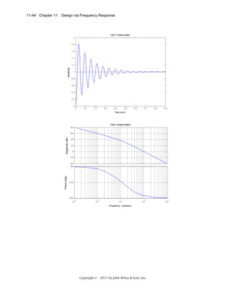
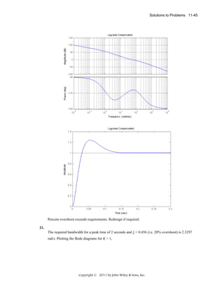
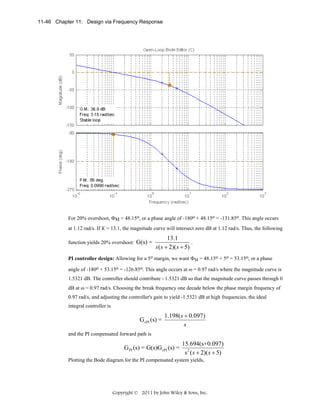
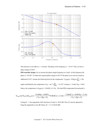
![Solutions to Problems 11-49
22.
Program:
%Input system
numg1=1;
deng1=poly([0 -3 -6]);
G1=tf(numg1,deng1);
[numg2,deng2]=pade(0.5,5);
G2=tf(numg2,deng2);
'G(s)=G1(s)G2(s)'
G=G1*G2;
Gzpk=zpk(G)
Tu=feedback(G,1);
step(Tu)
title('K = 1')
%Percent Overshoot to Damping Ratio to Phase Margin
Po=input('Type %OS ');
z=(-log(Po/100))/(sqrt(pi^2+log(Po/100)^2));
Pm=atan(2*z/(sqrt(-2*z^2+sqrt(1+4*z^4))))*(180/pi);
fprintf('nPercent Overshoot = %g',Po)
fprintf(', Damping Ratio = %g',z)
fprintf(', Phase Margin = %g',Pm)
%Get Bode data
bode(G)
title('K = 1')
pause
w=0.1:0.01:100;
[M,P]=bode(G,w);
Ph=-180+Pm;
for i=1:1:length(P);
if P(i)-Ph<=0;
M=M(i);
K=1/M;
Copyright © 2011 by John Wiley & Sons, Inc.](https://image.slidesharecdn.com/solutionscontrolsystemsengineeringbynormannice6ed-130502172814-phpapp02-131105052456-phpapp01/85/Solutions-control-system-sengineering-by-normannice-6ed-130502172814-phpapp02-779-320.jpg)
![Solutions to Design Problems 11-55
b.
1
-K-
0.005
140625
s+0.005
Constant
Gain
Transfer Fcn
v([1 2.67],[1 10
Transport
Delay
The figure shows a %OS slightly smaller than 15%.
Copyright © 2011 by John Wiley & Sons, Inc.
Transfer Fcn1
Scope](https://image.slidesharecdn.com/solutionscontrolsystemsengineeringbynormannice6ed-130502172814-phpapp02-131105052456-phpapp01/85/Solutions-control-system-sengineering-by-normannice-6ed-130502172814-phpapp02-785-320.jpg)
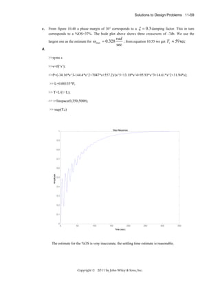
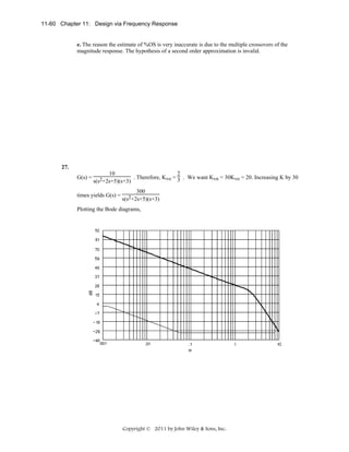
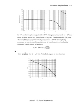
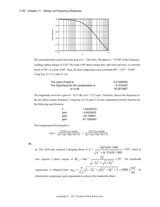
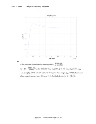
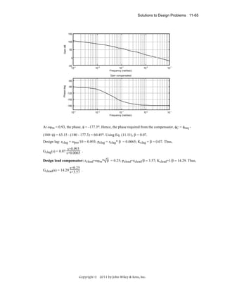
![11-66 Chapter 11: Design via Frequency Response
The lag-lead compensated Bode plot:
Gain dB
200
100
0
-100
10-4
10 -3
10 -2
10 -1
Frequency (rad/sec)
10 0
10 1
102
10 0
10 1
102
Lag-lead Compensated
Phase deg
-60
-90
-120
-150
-180
10-4
10 -3
10 -2
10 -1
Frequency (rad/sec)
b.
Program:
K=1926500;
numg=4.514e-6;
deng=[1 0.04348 0];
G=tf(numg,deng);
numgclag=0.07*[1 0.093];
dengclag=[1 0.0065];
Gclag=tf(numgclag,dengclag);
numgclead=14.29*[1 0.25];
dengclead=[1 3.57];
Gclead=tf(numgclead,dengclead);
Ge=K*G*Gclag*Gclead;
T=feedback(Ge,1);
step(T)
title('Lag-lead Compensated')
Copyright © 2011 by John Wiley & Sons, Inc.](https://image.slidesharecdn.com/solutionscontrolsystemsengineeringbynormannice6ed-130502172814-phpapp02-131105052456-phpapp01/85/Solutions-control-system-sengineering-by-normannice-6ed-130502172814-phpapp02-796-320.jpg)
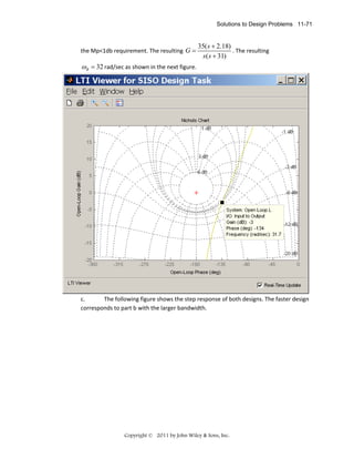
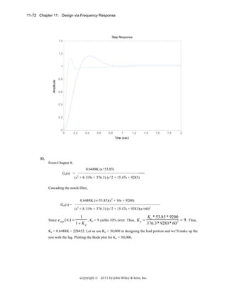

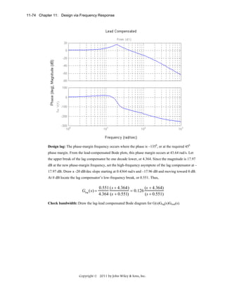
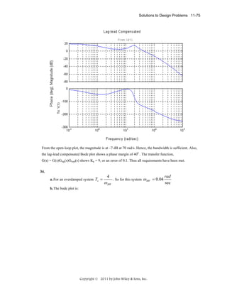
![Solutions to Design Problems 11-77
Step Response
1
0.9
0.8
0.7
Amplitude
0.6
0.5
0.4
0.3
0.2
0.1
0
0
20
40
60
80
100
120
140
160
180
Time (sec)
No further gain adjustments are necessary.
35.
a.
For a zero steady‐state error for step inputs and a steady‐state error for ramp
inputs ≤2 %, the required value of K may be found from:
eramp (∞) =
1
K ( s + 0 .6 )
≤ 0.02 , where K v = lim sG ( s ) = lim
≥ 50 .
Kv
s →0
s → 0 ( s + 0.5858)
Hence: 0.6× K ≥ 50 ⇒ K ≥ 48.82
0.5858
The following MATLAB file was used to plot the Bode magnitude and phase plots for that system
and to obtain the response of the system, c(t), to a step input, r(t) = 4 u(t).
numg = [1 0.6];
deng = poly ([0 -0.5858]);
G = 48.82*tf(numg, deng);
Copyright © 2011 by John Wiley & Sons, Inc.](https://image.slidesharecdn.com/solutionscontrolsystemsengineeringbynormannice6ed-130502172814-phpapp02-131105052456-phpapp01/85/Solutions-control-system-sengineering-by-normannice-6ed-130502172814-phpapp02-807-320.jpg)
![Solution to Case Study Challenge 12-5
e.
Program:
'Controller'
A=[0 1 0;0 -1.32 0.8;0 0 -100];
B=[0;0;2000];
C=[0.2 0 0];
D=0;
pos=input('Type desired %OS ');
Ts=input('Type desired settling time
');
z=(-log(pos/100))/(sqrt(pi^2+log(pos/100)^2));
wn=4/(z*Ts);
%Calculate required natural
%frequency.
[num,den]=ord2(wn,z);
%Produce a second-order system that
%meets the transient response
%requirements.
r=roots(den);
%Use denominator to specify dominant
%poles.
poles=[r(1) r(2) 10*real(r(1))];
%Specify pole placement for all
%poles.
K=acker(A,B,poles)
'Observer'
pos=input('Type desired %OS ');
z=(-log(pos/100))/(sqrt(pi^2+log(pos/100)^2));
wn=10*wn
%Calculate required natural
%frequency.
[num,den]=ord2(wn,z);
%Produce a second-order system that
%meets the transient response
%requirements.
r=roots(den);
%Use denominator to specify dominant
%poles.
poles=[r(1) r(2) 10*real(r(1))];%Specify pole placement for all
%poles.
l=acker(A',C',poles)'
Computer response:
ans =
Controller
Type desired %OS 15
Type desired settling time
2
K =
0.1871
0.0406
-0.0387
ans =
Observer
Type desired %OS
10
wn =
38.6899
l =
1.0e+006 *
0.0009
-0.0286
5.5691
Copyright © 2011 by John Wiley & Sons, Inc.](https://image.slidesharecdn.com/solutionscontrolsystemsengineeringbynormannice6ed-130502172814-phpapp02-131105052456-phpapp01/85/Solutions-control-system-sengineering-by-normannice-6ed-130502172814-phpapp02-817-320.jpg)
![12-6 Chapter 12: Design via State Space
ANSWERS TO REVIEW QUESTIONS
1. Both dominant and non-dominant poles can be specified with state-space design techniques.
2. Feedback all state variables to the plant's input through a variable gain for each. Decide upon a closedloop characteristic equation that has a pole configuration to yield a desired response. Write the
characteristic equation of the actual system. Match coefficients and solve for the values of the variable
gains.
3. Phase-variable form
4. The control signal developed by the controller must be able to affect every state variable.
5. If the signal-flow diagram is in the parallel form, which leads to a diagonal system matrix, controllability
can be determined by inspection by seeing that all state variables are fed by the control signal.
6. The system is controllable if the determinant of the controllability matrix is non-zero.
7. An observer is a system that estimates the state variables using information from the output of the actual
plant.
8. If the plant's state-variables are not accessible, or too expensive to monitor
9. An observer is a copy of the plant. The difference between the plant's output and the observer's output is
fed back to each of the derivatives of the observer's state variables through separate variable gains.
10. Dual phase-variable
11. The characteristic equation of the observer is derived and compared to a desired characteristic equation
whose roots are poles that represent the desired transient response. The variable gains of each feedback
path are evaluated to make the coefficients of the observer's characteristic equation equal the coefficients of
the desired characteristic equation.
12. Typically, the transient response of the observer is designed to be much faster than that of the
controller. Since the observer emulates the plant, we want the observer to estimate the plant's states rapidly.
13. Det[A-BK], where A is the system matrix, B is the input coupling matrix, and K is the controller.
14. Det[A-LC], where A is the system matrix, C is the output coupling matrix, and L is the observer.
15. The output signal of the system must be controlled by every state variable.
16. If the signal-flow diagram is in the parallel form, which leads to a diagonal system matrix, observability
can be determined by inspection by seeing that all state variables feed the output.
17. The system is observable if the determinant of the observability matrix is non-zero.
Copyright © 2011 by John Wiley & Sons, Inc.](https://image.slidesharecdn.com/solutionscontrolsystemsengineeringbynormannice6ed-130502172814-phpapp02-131105052456-phpapp01/85/Solutions-control-system-sengineering-by-normannice-6ed-130502172814-phpapp02-818-320.jpg)
![Solution to Problems 12-7
SOLUTIONS TO PROBLEMS
1.
i. G ( s ) =
( s + 3)
1
*( s + 3)
= 2
2
( s + 4)
s + 8s + 16
a.
b.
c.
•
0
1
⎡
⎤
⎡0⎤
x=⎢
⎥ x + ⎢1 ⎥ r ; y = [3 1] x
⎣ ⎦
⎣ −(k1 + 16) −(k2 + 8) ⎦
Copyright © 2011 by John Wiley & Sons, Inc.](https://image.slidesharecdn.com/solutionscontrolsystemsengineeringbynormannice6ed-130502172814-phpapp02-131105052456-phpapp01/85/Solutions-control-system-sengineering-by-normannice-6ed-130502172814-phpapp02-819-320.jpg)
![12-8 Chapter 12: Design via State Space
d.
T (s) =
s+3
s + (k2 + 8) s + (k1 + 16)
2
•
x1 = (−20 − 71.25k1 ) x1 − 71.25k2 x2 − 71.25k3 x3 + 71.25r
•
x 2 = 27.5k1 x1 + (−10 x2 + 27.5k2 ) x2 + 27.5k3 x3 − 27.5r
•
x3 = −6.25k1 x1 − 6.25k2 x2 − 6.25k3 x3 + 6.25r
−71.25k2
−71.25k3 ⎤
⎡(−20 − 71.25k1 )
⎡ 71.25 ⎤
⎢
⎥ ; B = ⎢ −27.5⎥ ; C = 1 1 1
27.5k1
(−10 x2 + 27.5k2 ) 27.5k3 ⎥
A=⎢
[
]
⎢
⎥
⎢
⎢ 6.25 ⎥
−6.25k1
−6.25k2
−6.25k3 ⎥
⎣
⎦
⎣
⎦
200( s 2 + 7 s + 25)
T (s) = 3
4 s + (120 + 285k1 − 110k2 + 25k3 ) s 2 + (800 + 2850k1 − 2200k2 + 750k3 ) s + 5000k3
e.
Part d. yields same result as i(d).
ii. G ( s ) =
s
1
= 2
*s
( s + 5)( s + 7) s + 12s + 35
a.
Copyright © 2011 by John Wiley & Sons, Inc.](https://image.slidesharecdn.com/solutionscontrolsystemsengineeringbynormannice6ed-130502172814-phpapp02-131105052456-phpapp01/85/Solutions-control-system-sengineering-by-normannice-6ed-130502172814-phpapp02-820-320.jpg)
![Solution to Problems 12-9
b.
c.
•
0
1
⎡
⎤
⎡0⎤
x=⎢
⎥ x + ⎢1 ⎥ r ; y = [ 0 1] x
⎣ ⎦
⎣ −(k1 + 35) −(k2 + 12) ⎦
d.
T (s) =
s
s + (k2 + 12) s + (k1 + 35)
2
e.
0
1
⎡
⎤
⎡0⎤
T ( s ) = C(sI − A) −1 B; A = ⎢
⎥ ; B = ⎢1 ⎥ ; C = [ 0 1]
⎣ ⎦
⎣ −(k1 + 35) −(k2 + 12) ⎦
which yields the same result as ii(d).
iii.
G(s) =
20s ( s + 7)
1
= 3
* (20s 2 +140s)
2
( s + 3)( s + 7)( s + 9) s + 19 s + 111s + 189
a.
Copyright © 2011 by John Wiley & Sons, Inc.](https://image.slidesharecdn.com/solutionscontrolsystemsengineeringbynormannice6ed-130502172814-phpapp02-131105052456-phpapp01/85/Solutions-control-system-sengineering-by-normannice-6ed-130502172814-phpapp02-821-320.jpg)
![12-10 Chapter 12: Design via State Space
b.
c.
0
1
0
⎡
⎤
⎡0 ⎤
⎢
⎥ x + ⎢0 ⎥ r ; y = 0 140 20 x
x=⎢
0
0
1
[
]
⎥
⎢ ⎥
⎢ −(k1 + 189) −(k2 + 111) −(k3 + 19) ⎥
⎢1 ⎥
⎣
⎦
⎣ ⎦
•
d.
T (s) =
20 s( s + 7)
s + (k3 + 19) s + (k2 + 111) s + (k1 + 189)
3
2
e.
0
1
0
⎡
⎤
⎡0⎤
⎢
⎥ ; B = ⎢0 ⎥ ; C = 0 140 20
T ( s ) = C(sI − A) B; A = ⎢
0
0
1
[
]
⎥
⎢ ⎥
⎢ −(k1 + 189) −(k2 + 111) −(k3 + 19) ⎥
⎢1 ⎥
⎣
⎦
⎣ ⎦
−1
which yields the same result as iii(d).
iv.
G ( s) =
30( s + 2)( s + 3)
1
= 3
* (30s 2 + 150 s + 180)
2
( s + 4)( s + 5)( s + 6) s + 15s + 74s + 120
Copyright © 2011 by John Wiley & Sons, Inc.](https://image.slidesharecdn.com/solutionscontrolsystemsengineeringbynormannice6ed-130502172814-phpapp02-131105052456-phpapp01/85/Solutions-control-system-sengineering-by-normannice-6ed-130502172814-phpapp02-822-320.jpg)
![Solution to Problems 12-11
a.
b.
c.
0
1
0
⎡
⎤
⎡0⎤
⎢
⎥ x + ⎢0 ⎥ r ; y = 180 150 30 x
x=⎢
0
0
1
[
]
⎥
⎢ ⎥
⎢ −(k1 + 120) −(k2 + 74) −( k3 + 15) ⎥
⎢1 ⎥
⎣
⎦
⎣ ⎦
•
Copyright © 2011 by John Wiley & Sons, Inc.](https://image.slidesharecdn.com/solutionscontrolsystemsengineeringbynormannice6ed-130502172814-phpapp02-131105052456-phpapp01/85/Solutions-control-system-sengineering-by-normannice-6ed-130502172814-phpapp02-823-320.jpg)
![12-12 Chapter 12: Design via State Space
d.
T (s) =
30 s 2 + 150s + 180
s 3 + (k3 + 15) s 2 + (k2 + 74) s + (k1 + 120)
e.
0
1
0
⎡
⎤
⎡0⎤
⎢
⎥ ; B = ⎢ 0 ⎥ ; C = 180 150 30
T ( s ) = C(sI − A) B; A = ⎢
0
0
1
[
]
⎥
⎢ ⎥
⎢ −(k1 + 120) −(k2 + 74) −(k3 + 15) ⎥
⎢1 ⎥
⎣
⎦
⎣ ⎦
−1
which yields the same result as iv(d).
v. G ( s ) =
s 2 + 8s + 15
1
= 4
* (s 2 + 8s + 15)
2
2
3
2
(s + 4 s + 10)(s + 3s + 12) s + 7 s + 34 s + 78s + 120
a.
b.
Copyright © 2011 by John Wiley & Sons, Inc.](https://image.slidesharecdn.com/solutionscontrolsystemsengineeringbynormannice6ed-130502172814-phpapp02-131105052456-phpapp01/85/Solutions-control-system-sengineering-by-normannice-6ed-130502172814-phpapp02-824-320.jpg)
![Solution to Problems 12-13
c.
0
1
0
0
⎡
⎤
⎡0 ⎤
⎢
⎥
⎢ ⎥
•
0
0
1
0
⎢
⎥ x + ⎢0 ⎥ r ; y = [15 8 1 0] x
x=
⎢
⎥
⎢0 ⎥
0
0
0
1
⎢
⎥
⎢ ⎥
⎢ −(k1 + 120) −(k2 + 78) −(k3 + 34) −(k4 + 7) ⎥
⎣1 ⎦
⎣
⎦
d.
T (s) =
s 2 + 8s + 15
s 4 + (k4 + 7) s 3 + (k3 + 34) s 2 + (k2 + 78) s + (k1 + 120)
e.
0
1
0
0
⎡
⎤
⎡0 ⎤
⎢
⎥
⎢ ⎥
0
0
1
0
⎥ ; B = ⎢0 ⎥ ; C = [15 8 1 0]
T ( s ) = C(sI − A) −1 B; A = ⎢
⎢
⎥
⎢0 ⎥
0
0
0
1
⎢
⎥
⎢ ⎥
⎢ −(k1 + 120) −(k2 + 78) −(k3 + 34) −(k4 + 7) ⎥
⎣1 ⎦
⎣
⎦
which yields the same result as v(d).
2.
i
a. The output is
Since,
Copyright © 2011 by John Wiley & Sons, Inc.](https://image.slidesharecdn.com/solutionscontrolsystemsengineeringbynormannice6ed-130502172814-phpapp02-131105052456-phpapp01/85/Solutions-control-system-sengineering-by-normannice-6ed-130502172814-phpapp02-825-320.jpg)
![12-14 Chapter 12: Design via State Space
&
&
y = (30 s 2 + 270s + 420) x1 = 30 &&1 + 270 x1 + 420 x1 = 30 x2 + 270 x2 + 420 x1
x
= 30(−5 x2 + x3 ) + 270 x2 + 420 x1 = 420 x1 + 120 x2 + 30 x3
b.
⎡ 0
T ( s ) = C(sI − A) B; A = ⎢ 0
⎢
⎢ − k1
⎣
−1
T (s) =
1
⎤
⎡0⎤
⎥ ; B = ⎢0 ⎥ ; C = 420 120 30
1
[
]
⎥
⎢ ⎥
⎢1 ⎥
−(k3 + 3) ⎥
⎦
⎣ ⎦
0
−5
− k2
30( s + 2)( s + 7)
s (k3 + 8) s 2 + (5k3 + k2 + 15) s + k1
3
ii
a.
1
u
1
5
r
1
s
x3
1
s
1
-2
1
s
3
x
1
7
-10
-k
2
-k
1
⎡ 0
T(s) = C(sI − A) B; A = ⎢ 0
⎢ −k
⎣
−1
1
=
1
-2
-k 3
b.
x2
1
0
−k 2
⎤
0
⎡0 ⎤
⎥; B = ⎢ 0 ⎥; C = [-3 1 1]
1
⎢5 ⎥
−(5k 3 + 2)⎥
⎣ ⎦
⎦
5(s2 + 3s + 7)
s3 + (5k 3 + 4)s2 + (10k 3 + k 2 + 14)s + (50k 3 + k 1 + 20)
3.
Copyright © 2011 by John Wiley & Sons, Inc.
y](https://image.slidesharecdn.com/solutionscontrolsystemsengineeringbynormannice6ed-130502172814-phpapp02-131105052456-phpapp01/85/Solutions-control-system-sengineering-by-normannice-6ed-130502172814-phpapp02-826-320.jpg)
![Solution to Problems 12-15
i
a.
G ( s) =
50( s 2 + 7 s + 25) 6.25 27.5 71.25
=
−
+
s ( s + 10)( s + 20)
s
s + 10 s + 20
b. Writing the state equations:
•
x1 = −20 x1 + 71.25u
•
x 2 = −10 x2 − 27.5u
•
x3 = 6.25u
But, u = -k1x1 - k2x2 - k3x3 + r . Substituting into the state equations,
•
x1 = (−20 − 71.25k1 ) x1 − 71.25k2 x2 − 71.25k3 x3 + 71.25r
•
x 2 = 27.5k1 x1 + (−10 x2 + 27.5k2 ) x2 + 27.5k3 x3 − 27.5r
•
x3 = −6.25k1 x1 − 6.25k2 x2 − 6.25k3 x3 + 6.25r
Therefore, T(s) = C(sI - A)-1B, where
−71.25k2
−71.25k3 ⎤
⎡(−20 − 71.25k1 )
⎡ 71.25 ⎤
⎢
⎥ ; B = ⎢ −27.5⎥ ; C = 1 1 1
A=⎢
27.5k1
(−10 x2 + 27.5k2 ) 27.5k3 ⎥
[
]
⎢
⎥
⎢
⎢ 6.25 ⎥
−6.25k1
−6.25k2
−6.25k3 ⎥
⎣
⎦
⎣
⎦
Hence,
Copyright © 2011 by John Wiley & Sons, Inc.](https://image.slidesharecdn.com/solutionscontrolsystemsengineeringbynormannice6ed-130502172814-phpapp02-131105052456-phpapp01/85/Solutions-control-system-sengineering-by-normannice-6ed-130502172814-phpapp02-827-320.jpg)
![12-16 Chapter 12: Design via State Space
T (s) =
200( s 2 + 7 s + 25)
4s 3 + (120 + 285k1 − 110k2 + 25k3 ) s 2 + (800 + 2850k1 − 2200k2 + 750k3 ) s + 5000k3
ii
a.
G(s) =
50(s + 3)(s + 4)
50
300 300
=
−
+
(s + 5)(s + 6)(s + 7) s + 5 s + 6 s + 7
x1
400
950
-30
-5
1
-k 1
x2
1
100
-300
1
-15
-6
9
-k 2
400
300
1
x3
-k 3
9
-7
b. Writing the state equations:
•
x1 = −5x1 + 50u
•
x2 = −6x 2 − 300u
•
x3 = −7x3 + 300u
But,
u = −k1 x1 − k2 x 2 − k 3 x3 + r
Substituting into the state equations, collecting terms, and converting to vector-matrix form yields
−50k2
−50k 3 ⎤
⎡ −(5 + k1 )
⎡ 50 ⎤
x = ⎢ 300k1
(300k2 − 6) 300k3 ⎥ x + ⎢ −300 ⎥r
⎢−(300k1 + 7)
⎢ 300 ⎥
−300k2
300k3 ⎥
⎣
⎦
⎣
⎦
•
y = [1 1 1]x
Therefore, T(s) = C(sI - A)-1B, or
Copyright © 2011 by John Wiley & Sons, Inc.](https://image.slidesharecdn.com/solutionscontrolsystemsengineeringbynormannice6ed-130502172814-phpapp02-131105052456-phpapp01/85/Solutions-control-system-sengineering-by-normannice-6ed-130502172814-phpapp02-828-320.jpg)
![Solution to Problems 12-17
T (s) =
50s2 + 1750s + (6900 − 88200k1 )
3
2
s + (300k3 − 300k 2 + k1 + 11)s + 2(1475k3 − 750k 2 + 3k1 − 7350k3 k1 + 7350k2 k1 + 15)s
+ 300k3 (23 − 294k1 )
4.
The plant is given by
G( s) =
20
20
= 3
2
( s + 2)( s + 4)( s + 8) s + 14 s + 56s + 64
The characteristic polynomial for the plant with phase-variable state feedback is
s 3 + ( k3 + 14) s 2 + ( k2 + 56) s + ( k1 + 64) = 0
The desired characteristic equation is
( s + 53.33)( s 2 + 10.67 s + 106.45) = s 3 + 64s 2 + 675.48s + 5676.98
based upon 15% overshoot, Ts = 0.75 second, and a third pole ten times further from the imaginary
axis than the dominant poles. Comparing the two characteristic equations,
k1 = 5612.98, k2 = 619.48, and k3 = 50 .
5.
a. The system in controller canonical form is:
⎡− a n − 1
⎢ 1
A=⎢
⎢ M
⎢ 0
⎣
−a n− 2 L − a1
0
L
0
M
M
M
0
L
1
− a0 ⎤
⎡1 ⎤
⎢0 ⎥
0 ⎥
⎥;B = ⎢ ⎥;C = c
1
M ⎥
⎢0 ⎥
⎢0 ⎥
0 ⎥
⎦
⎣ ⎦
[
c2
c3
c4
]
The characteristic equation of the plant is:
sn + an-1sn-1 + . . . + a1s + a0 = 0
Forming the closed-loop system by feeding back each state variable and the input to u forming
u = -Kx + r
where
K = [k1 k2 . . . kn]
and substituting u into the state equation, we obtain
.
x = Ax + B u = ( A − BK )x + B r
Forming A - BK:
Copyright © 2011 by John Wiley & Sons, Inc.](https://image.slidesharecdn.com/solutionscontrolsystemsengineeringbynormannice6ed-130502172814-phpapp02-131105052456-phpapp01/85/Solutions-control-system-sengineering-by-normannice-6ed-130502172814-phpapp02-829-320.jpg)
![12-18 Chapter 12: Design via State Space
⎡ −(a n− 1+ k1 ) −(a n− 2 + k 2 ) L −(a1 + k n −1 ) −(a 0 + k n )⎤
⎥
⎢
L
0
0
1
0
A − BK = ⎢
⎥
M
M
M
M
M
⎥
⎢
0
0
L
1
0
⎦
⎣
The characteristic equation is:
sn + (an-1 + k1)sn-1 + (an-2 + k2). . . + (a1 + kn-1)s + (a0 + kn) = 0
Assuming a desired characteristic equation,
sn + dn-1sn-1 + dn-2sn-2+ . . . + d2s2 + d1s + d0 = 0
Equating coefficients,
di = ai + kn-i ; i = 0, 1, 2, ... n-1
from which
kn-i = di – ai
(1)
b. The desired characteristic equation is
s + 15.9s + 136.08s + 413.1 = 0
3
2
the characteristic equation of the plant is
s + 5s + 4s + 0 = 0
3
2
Using Eq. (1) above, k3-i = di – ai. Therefore, k3 = d0 – a0 = 413.1 – 0 = 413.1; k2 = d1 – a1 = 136.08 –
4 = 132.08; k1 = d2 – a2 = 15.9 – 5 = 10.9. Hence,
K = [10.9 132.08 413.1]
6.
Using Eqs. (4.39) and (4.34) to find ζ = 0.5169 and ωn = 7.3399, respectively. Factoring the
denominator of Eq. (4.22), the required poles are -3.7942 ± j6.2832. We place the third pole at -2 to
cancel the open loop zero. Multiplying the three closed-loop pole terms yields the desired
characteristic equation:
100s2 + 2200s + 4000
, the controller
s3 + 9.5885s2 + 69.0516s + 107.7493 = 0. Since G(s) = 3
s + 8 s2 + 19 s + 12
⎡− 8 − 19 − 12⎤
⎡1 ⎤
⎢
⎢ ⎥
⎥
0
0 ⎥ ; B = ⎢0 ⎥ ; C = [100 2200 4000]. The first row of A
canonical form is A = ⎢ 1
⎢0
⎢0 ⎦
⎥
1
0 ⎦
⎣
⎣ ⎥
contains the coefficients of the characteristic equation. Thus comparing the first row of A to the
desired characteristic equation and using the results of Problem 5, k1 = -(9.5885 - 8) = 1.5885;
k2 = -(69.0516 - 19) = 50.0516; and k3 = -(107.7493 - 12) = 95.7493.
7.
The plant is given by
Copyright © 2011 by John Wiley & Sons, Inc.](https://image.slidesharecdn.com/solutionscontrolsystemsengineeringbynormannice6ed-130502172814-phpapp02-131105052456-phpapp01/85/Solutions-control-system-sengineering-by-normannice-6ed-130502172814-phpapp02-830-320.jpg)
![Solution to Problems 12-21
a.
-2
A =
0
1
0
;B =
0
-2
0
0
0
-3
0
1
M
1
-5
1
=
1
-2
4
1
;C
-3
9
; det C
= 0 ; system is uncontrollable
M
b.
-2
1
0
0
-2
0
0
0
-3
-4
1
0
0
0
1
0
0
-3
-4
1
0
A =
0
;B =
1
0
=
M
1
1
-4
1
-2
4
1
;C
-3
9
; det C
M
= -1 ; system is controllable
c.
A =
0
;B =
2
0
-7
1
-3
-3
9
-4
17
0
1
-8
1
1
2
1
M
=
2
1
;C
-8
44
; det C
= 7 ; system is controllable
M
d.
A =
1
;B =
0
0
1
-5
0
0
-3
;C
=
M
1
; det C
M
= -5 ; system is controllable
e.
0
A =
-6
1
-5
1
; B =
; C
-2
M
=
1
-2
-2
4
1
0
-4
0
16
0
1
-6
36
; det C
M
=0 ; sy stem is u n co n tro llab le
f.
0
-5
0
0
0
A =
-4
0
0
-6
;B =
1
0
; C
1
M
=
; det C
M
This system can also be determined uncontrollable by inspection.
12.
Program:
'(d)'
A=[-4 1 0;0 0 1;-5 0 -3]
B=[1;0;1]
Cm=ctrb(A,B)
Rank=rank(Cm)
pause
'(f)'
A=[-4 0 0;0 -5 0;0 0 -6]
B=[1;0;1]
Cm=ctrb(A,B)
Rank=rank(Cm)
Copyright © 2011 by John Wiley & Sons, Inc.
=0 ; system is uncontrollable](https://image.slidesharecdn.com/solutionscontrolsystemsengineeringbynormannice6ed-130502172814-phpapp02-131105052456-phpapp01/85/Solutions-control-system-sengineering-by-normannice-6ed-130502172814-phpapp02-833-320.jpg)
![Solution to Problems 12-23
C Mz
⎡0
⎢
= ⎢0
⎢1
⎣
1 ⎤
⎡1
⎥
⎢
1 − 3⎥ . For the controller canonical form, C Mcc = ⎢0
⎢0
−1 1 ⎥
⎦
⎣
−8
1
0
0
47⎤
⎥
−8⎥ . The transformation
1⎥
⎦
⎡0 0 1 ⎤
⎢
⎥
matrix is, P = CMzCMcc-1 = ⎢0 1 5 ⎥ . Comparing the first row of Acc with the desired
⎢
⎥
⎣1 7 10⎦
characteristic equation, Eq. (12.50), Kcc = [ -2
Kz = KccP-1 = [-20
10
-4
10]. Transforming back to the original system,
-2].
14.
Drawing the signal-flow diagram for the plant in cascade form yields
u
1
s
1
z3
1
s
1
-10
z2
1
1
s
1
z1 6
y
-3
-8
Writing the A and B matrices for the z system,
Az
-3
0
0
1
-8
0
Bz
0
0
1
0
1
-10
Writing the A and B matrices for the x (phase-variable) system,
Ax
0
0
-240
1
0
-134
Bx
0
0
1
0
1
-21
Phase-Variable Form
From the phase variable from, the characteristic polynomial is s3 + 21s2 + 134s + 240.
Finding the controllability matrices and their determinants for the z and x systems shows that there is
controllability,
CMz
Controllability Matrix of z
CMx
Controllability Matrix of x
0
0
1
0
0
1
0
1
-18
0
1
-21
1
-10
100
1
-21
307
Det(CMz)
-1
Det(CMx)
-1
Copyright © 2011 by John Wiley & Sons, Inc.](https://image.slidesharecdn.com/solutionscontrolsystemsengineeringbynormannice6ed-130502172814-phpapp02-131105052456-phpapp01/85/Solutions-control-system-sengineering-by-normannice-6ed-130502172814-phpapp02-835-320.jpg)
![12-24 Chapter 12: Design via State Space
Using Eq. (12.39), the transformation matrix P and its inverse are found to be
Transformation Matrix z=Px
P
PINV
1
0
0
1.00
0.00
0.00
3
1
0
-3.00
1.00
0.00
24
11
1
9.00
-11.00
1.00
Using the given transient requirements, and placing the third closed-loop pole over the zero at -6
yields the following desired closed-loop characteristic polynomial:
(s2 + 8s + 45.78)(s + 6) = s3 + 14s2 + 93.78s + 274.68
Using the phase-variable system with state feedback the characteristic polynomial is
s3 + (k3 + 21)s2 + (k2 + 134)s + (k1 + 240)
Equating the two characteristic polynomials yields the state feedback vector for the x system as
Kx
34.68
Controller for x
-40.22
-7
Using Eq. (12.42),
Kz
92.34
Controller for z
36.78
-7
15.
Program:
A=[-3 1 0;0 -8 1;0 0 -10];
%Generate system matrix A
B=[0;0;1];
%Generate input coupling matrix B
C=[3 1 0];
%Generate output coupling matrix C
D=0;
%Generate matrix D
Po=10;
%Input desired percent overshoot
Ts=1;
%Input desired settling time
z=(-log(Po/100))/(sqrt(pi^2+log(Po/100)^2));
%Calculate required damping ratio
wn=4/(z*Ts);
%Calculate required natural
%frequency
[num,den]=ord2(wn,z);
%Produce a second-order system that
%meets transient requirements
r=roots(den);
%Use denominator to specify
%dominant poles
poles=[r(1) r(2) -6];
%Specify pole placement for all
%poles.
%A few tries at the the third-pole
%value shows T(s) with a closed%loop zero at -7.
%Thus, choose the third pole to
%cancel this zero.
K=acker(A,B,poles)
%Calculate controller gains in z%system
Anew=A-B*K;
%Form compensated A matrix
Bnew=B;
%Form compensated B matrix
Cnew=C;
%Form compensated C matrix
Dnew=D;
%Form compensated D matrix
[numt,dent]=ss2tf(Anew,Bnew,Cnew,Dnew);
%Form T(s)
'T(s)'
%Display label
T=tf(numt,dent)
%Display T(s)
poles=pole(T)
%Display poles of T(s)
Copyright © 2011 by John Wiley & Sons, Inc.](https://image.slidesharecdn.com/solutionscontrolsystemsengineeringbynormannice6ed-130502172814-phpapp02-131105052456-phpapp01/85/Solutions-control-system-sengineering-by-normannice-6ed-130502172814-phpapp02-836-320.jpg)
![12-26 Chapter 12: Design via State Space
Using Eq. (12.39), the transformation matrix P and its inverse are found to be
P
6.85712
6
-6.85704
Transformation Matrix z=Px
1.542852
0.085714
2.6
0.2
-3.14281
-0.28571
PINV
0.33
-1.00
3.00
-0.50
4.00
-32.00
-0.25
2.50
-25.00
Using the given transient requirements, and placing the third closed-loop pole over the zero at -6
yields the following desired closed-loop characteristic polynomial:
(s2 + 8s + 45.78)(s + 6) = s3 + 14s2 + 93.78s + 274.68
Using the phase-variable system with state feedback the characteristic polynomial is
s3 + (k3 + 21)s2 + (k2 + 134)s + (k1 + 240)
Equating the two characteristic polynomials yields the state feedback vector for the x system as
Kx
34.7062
Controller for x
-40.2156
-7
Using Eq. (12.42),
Controller for z
45.7845
Kz
30.78443595
65.78543678
17.
Draw signal-flow diagram showing state variables, z, at the output of each subsystem and the state
variables, w, at the output of the integrators.
u
1
1
s
-3
Recognizing that
z3
1
s
1
1
z1 6
z2 1
1
s
w2
w3
-8
-10
z1
1
y
w1
z2 = 6 w2 − 8w2 + w3 = −2w2 + w3 , we can write the state equations for w as
⎡ −10 −2 1 ⎤
⎡ 0⎤
w = ⎢ 0 −8 1 ⎥ w + ⎢ 0⎥ u
⎢ 0
⎢1 ⎥
0 −3⎥
⎦
⎣
⎣ ⎦
•
y = [1 0 0]w
Writing the relationship between z and w yileds
Copyright © 2011 by John Wiley & Sons, Inc.](https://image.slidesharecdn.com/solutionscontrolsystemsengineeringbynormannice6ed-130502172814-phpapp02-131105052456-phpapp01/85/Solutions-control-system-sengineering-by-normannice-6ed-130502172814-phpapp02-838-320.jpg)
![12-28 Chapter 12: Design via State Space
Equating the two characteristic polynomials yields the state feedback vector for the x system as
Kx
34.68
Controller for x
-40.22
-7
Using Eq. (12.42),
Kz
65.78
Controller for z
-10
3
18.
Using Eqs. (4.39) and (4.34) to find ζ = 0.5169 and ωn = 18.3498 respectively. Factoring the
denominator of Eq. (4.22), the required poles are -9.4856 ± j15.708. We place the third pole 10 times
further at -94.856. Multiplying the three closed-loop pole terms yields the desired characteristic
equation: s3 + 114s2 + 2136s + 31940 = 0. Representing the plant in parallel form:
A par
⎡0 0 0 ⎤
⎡ 2.222 ⎤
⎢0 −5 0 ⎥ B = ⎢ −5 ⎥
=
⎥ ; Cpar = [1 1 1]. Using Eq. (12.26),
⎢
⎥ ; par ⎢
⎢ 2.778⎥
⎢ 0 0 −9 ⎥
⎣
⎦
⎣
⎦
CMpar
0 ⎤
⎡ 2.222 0
= ⎢ −5
−125 ⎥ , which is controllable since the determinant is 5555.4. Since
25
⎢
⎥
⎢ 2.778 −25 225.018⎥
⎣
⎦
⎡ −14 −45 0⎤
⎢
100
0 0⎥ ; B
, the controller canonical form is A cc = ⎢ 1
G( s) = 3
⎥ cc
s + 14 s 2 + 45s
1 0⎥
⎢ 0
⎣
⎦
⎡1 ⎤
⎢ ⎥
= ⎢0 ⎥ ;
⎢0 ⎦
⎣ ⎥
⎡1 −14 151 ⎤
⎢
1 −14 ⎥ , which is controllable since the
C = [0 0 100 ]. Using Eq. (12.26), CMcc = ⎢ 0
⎥
1 ⎥
⎢0 0
⎣
⎦
determinant is 1. The first row of Acc contains the coefficients of the characteristic equation.
Comparing the first row of Acc to the desired characteristic equation and using the results of Problem
5, (14 + k1) = 114; (45 + k2)= 2136; and (0 + k3)= 31940. Hence Kcc =[31940 2091 110]. The
⎡ 2.222 31.108 99.99 ⎤
⎢
0 ⎥ . Transforming back to
−45
transformation matrix is, P = CMparCMcc-1 = ⎢ −5
⎥
0 ⎥
⎢ 2.778 13.89
⎣
⎦
the original system, Kpar = KccP-1 = [1.1 7882 25682].
Copyright © 2011 by John Wiley & Sons, Inc.](https://image.slidesharecdn.com/solutionscontrolsystemsengineeringbynormannice6ed-130502172814-phpapp02-131105052456-phpapp01/85/Solutions-control-system-sengineering-by-normannice-6ed-130502172814-phpapp02-840-320.jpg)
![Solution to Problems 12-29
19.
a.
>> A=[-0.014 0 -1.4 0 0; 0.023 -0.023 -0.023 0 0; 0.134 0.67 -0.67 0.38 0.003264; 0 0 0.06 -0.06 0;
0 0 0.0017 0 -0.001];
>> B = [1;0;0;0;0];
>> rank(ctrb(A,B))
ans =
5
The controllability matrix has full rank so the system is controllable.
b.
>> [P,Ad]=jordan(A) % P is the similarity transformation matrix used for diagonalization, Ad the
diagonalized A matrix
P=
-0.0000 + 0.0000i 1.3181 + 0.1838i 0.0446
-1.6808
1.3181 - 0.1838i
-0.0000 + 0.0000i -0.0336 - 0.0948i -0.0286
0.0958
-0.0336 + 0.0948i
0.0000 - 0.0000i 0.1916 - 0.1798i 0.0014
-0.3845
0.1916 + 0.1798i
0.0000 - 0.0000i -0.0605 - 0.0176i 0.0370
0.0841
-0.0605 + 0.0176i
0.0012 - 0.0000i -0.0016 - 0.0002i -0.0000
0.0020
-0.0016 + 0.0002i
Copyright © 2011 by John Wiley & Sons, Inc.](https://image.slidesharecdn.com/solutionscontrolsystemsengineeringbynormannice6ed-130502172814-phpapp02-131105052456-phpapp01/85/Solutions-control-system-sengineering-by-normannice-6ed-130502172814-phpapp02-841-320.jpg)
![Solution to Problems 12-31
OMz
1
-10
79
Observability Matrix of z
0
1
-10
0
0
1
1
Det(OMz)
Using the given transient requirements, and placing the third closed-loop pole 10 times further from
the imaginary axis than the dominant poles yields the following desired characteristic polynomial:
(s + 300)(s2 + 60s + 5625) = s3 + 360s2 + 23625s + 1687500
Equating this polynomial to Eq. (12.67), yields the observer gains as:
Lz
350
23604
1687500
21.
Observer for z
Using Eqs. (4.39) and (4.34) to find ζ = 0.5912 and ωn = 19.4753 respectively. Factoring the
denominator of Eq. (4.22), the required poles are -11.513 ± j15.708. We place the third pole 20 times
further at –230.26. Multiplying the three closed-loop pole terms yields the desired characteristic
equation: s3 + 253.28s2 + 5681.19s + 87334.19 = 0.
⎡ −25 1 0 ⎤
⎡0⎤
A oc = ⎢ −171 0 1 ⎥ ; B = ⎢ 0 ⎥ ;
Representing the plant in observer canonical form:
⎢
⎥ oc
⎢ −315 0 0 ⎥
⎢10 ⎥
⎣
⎦
⎣ ⎦
Coc = [1 0 0]. The first column of Aoc contains the coefficients of the characteristic equation.
Comparing the first column of Aoc to the desired characteristic equation and using Eq. (12.67), l1 =
253.28 - 25 = 228.28; l2 = 5681.19 - 171 = 5510.19; and l3 = 87334.19 - 315 = 87019.19. Hence,
Loc = [228.28 5510.19 87019.19]T.
22.
The A, L, and C matrices for the phase-variable system are:
0 ⎤
⎡0 1
A = ⎢0 0
1 ⎥
⎢ 0 −21 −10⎦
⎥
⎣
C = [1 0 0 ]
Copyright © 2011 by John Wiley & Sons, Inc.](https://image.slidesharecdn.com/solutionscontrolsystemsengineeringbynormannice6ed-130502172814-phpapp02-131105052456-phpapp01/85/Solutions-control-system-sengineering-by-normannice-6ed-130502172814-phpapp02-843-320.jpg)
![12-32 Chapter 12: Design via State Space
⎡ l1 ⎤
L = ⎢ l2 ⎥
⎢l ⎦
⎣ ⎥
3
Hence,
⎡ λ + l1
λ − ( A − LC) = ⎢ l2
⎢ l
⎣
3
or
−1
⎤
λ
−1 ⎥
21 λ + 10⎥
⎦
0
λ − (A − LC) = λ3 + (10 + l1 )λ2 + (21+ 10l1 + l2 )λ + (21l1 + 10l2 + l3 )
From Problem 19, the desired characteristic polynomial is λ3 + 360λ2 + 23625λ + 1687500.
Equating coefficients yields:
10 + l1 = 360; (21+ 10 l1 + l2 ) = 23625; (21l1 + 10l2 + l3 ) = 1687500
Solving successively,
l1 = 350; l2 = 20104; l3 = 1479110
23.
The A, L, and C matrices for the phase-variable system are:
1 ⎤
⎡ 0
⎡ l1 ⎤
A=⎢
; C = [2 1]; L = ⎢ ⎥
⎣ −45 −14⎥
⎣l2 ⎦
⎦
Hence,
l1 − 1 ⎤
⎡ λ + 2l1
λ − (A − LC) = ⎢
⎣ 2l2 + 45 l2 + λ + 14⎥
⎦
or
λ2 + (2l1 + l2 + 14)λ + (2l2 − 17l1 + 45)
From the problem statement, the desired characteristic polynomial is λ2 + 144λ + 14400.
Equating coefficients yields,
(2l1 + l2 + 14) = 144; (2l2 − 17l1 + 45) = 14400
Solving simultaneously,
l1 = −671.2; l2 = 1472.4
24.
The A matrix for each part is given in the solution to Problem 11. Each observability matrix is
calculated from Eq. (12.79).
a.
Copyright © 2011 by John Wiley & Sons, Inc.](https://image.slidesharecdn.com/solutionscontrolsystemsengineeringbynormannice6ed-130502172814-phpapp02-131105052456-phpapp01/85/Solutions-control-system-sengineering-by-normannice-6ed-130502172814-phpapp02-844-320.jpg)
![Solution to Problems 12-33
b.
c.
d.
e.
f.
25.
Program:
'(a)'
A=[-2 0 1;0 -2 0;0 0 -3]
C=[5 5 5]
Om=obsv(A,C)
Rank=rank(Om)
'(f)'
A=[-4 0 0;0 -5 0;0 0 -6]
C=[1 1 1]
Om=obsv(A,C)
Rank=rank(Om)
%Form compensated A matrix
%Form compensated C matrix
%Form observability matrix
%Find rank of observability
%matrix
%Form
%Form
%Form
%Find
compensated A matrix
compensated C matrix
observability matrix
rank of observability
Computer response:
ans =
(a)
A =
-2
0
0
0
-2
0
1
0
-3
5
5
5
5
-10
20
5
-10
20
5
-10
20
C =
Om =
Rank =
1
ans =
(f)
Copyright © 2011 by John Wiley & Sons, Inc.](https://image.slidesharecdn.com/solutionscontrolsystemsengineeringbynormannice6ed-130502172814-phpapp02-131105052456-phpapp01/85/Solutions-control-system-sengineering-by-normannice-6ed-130502172814-phpapp02-845-320.jpg)
![Solution to Problems 12-35
To test observability, we write the observability matrices for both systems and show that both
observability matrices have non zero determinants. Using Eq. (12.79),
OMz
1
-20
400
Observability Matrix of z
0
1
-33
OMx
1
-38
1019
0
0
1
1
Det(OMz)
Observability Matrix of x
0
1
-38
0
0
1
1
Det(OMx)
Using Eq. (12.89), we obtain the transformation matrix, P, and its inverse as
Transformation Matrix z=Px
0
0
1
0
-5
1
P
1
-18
25
PINV
1.00
18.00
65.00
0.00
1.00
5.00
Using the characteristic polynomial given in the problem statement, the plant’s characteristic
equation, and Eq. (12.67), the observer for the observer canonical system is
Lx
562
39575
1498700
Observer for x
Using Eq. (12.92), the observer for the cascade system is found to be
Lz
562
29459
1314875
Observer for z
28.
Program:
A=[-20 1 0;0 -13 1;0 0 -5]
B=[0;0;1]
C=[1 0 0]
D=0
poles=roots([1 600 40000 1500000])
L=acker(A',C',poles);
'L'
L'
Computer response:
A =
-20
0
0
1
-13
0
0
1
-5
B =
0
0
Copyright © 2011 by John Wiley & Sons, Inc.
0.00
0.00
1.00](https://image.slidesharecdn.com/solutionscontrolsystemsengineeringbynormannice6ed-130502172814-phpapp02-131105052456-phpapp01/85/Solutions-control-system-sengineering-by-normannice-6ed-130502172814-phpapp02-847-320.jpg)
![12-38 Chapter 12: Design via State Space
⎡ − 18 1 0 ⎤
50
⎢
⎥
Since G(s) = 3
, the plant in observer canonical form is: A oc = ⎢ − 99 0 1 ⎥ ;
s + 18s2 + 99s + 162
⎢ −162 0 0 ⎦
⎥
⎣
⎡0⎤
⎡ 1
0
0⎤
⎢ ⎥
⎢
⎥
Boc = ⎢ 0 ⎥ ; Coc = [1 0 0]. Using Eq. (12.79), OMoc = ⎢− 18 1
0⎥ , which is observable since
⎢ ⎥
⎢
⎥
⎣50 ⎦
⎣ 225 − 18 1⎦
50
, the phase-variable form is
the determinant is 1. Since G(s) = 3
s + 18s2 + 99s + 162
A pv
⎡ 0
1
0 ⎤
⎡0 ⎤
⎢
⎥
⎢ ⎥
0
1 ⎥ ; Bpv = ⎢0 ⎥ ; C = [50 0 0 ]. Using Eq. (12.79),
=⎢ 0
⎢− 162 − 99 − 18⎥
⎢1 ⎦
⎣
⎦
⎣ ⎥
⎡50 0 0 ⎤
⎢
⎥
OMpv = ⎢ 0 50 0 ⎥ , which is observable since the determinant is 125000. The first column of
⎢0
0 50 ⎥
⎣
⎦
Aoc contains the negatives values of the coefficients of the characteristic equation. Comparing the
first column of Aoc to the desired characteristic equation and using Eq. (12.67), l1 = 960-18 = 942; l2
= 146313.746-99 = 146214.746; and l3 = 14650996.915-162= 14650834.915. Hence,
Loc = [942 146214.746 14650834.915]. The transformation matrix is,
⎡ 0. 02
0
0 ⎤
⎢
⎥
P = OMpv-1OMoc = ⎢−0. 36 0.02
0 ⎥
⎢
⎥
⎣ 4.5 − 0.36 0. 02⎦
Transforming back to the original system, Lpv = PLoc = [18.84 2585.175 244618.39]T.
31.
a.
Since both systems are in phase variable form it readily follows that:
det( sI − A 1 ) = s 2 + 3s + 2
and
det( sI − A 2 ) = s 3 + 6s 2 + 11s + 6
Copyright © 2011 by John Wiley & Sons, Inc.](https://image.slidesharecdn.com/solutionscontrolsystemsengineeringbynormannice6ed-130502172814-phpapp02-131105052456-phpapp01/85/Solutions-control-system-sengineering-by-normannice-6ed-130502172814-phpapp02-850-320.jpg)
![Solution to Problems 12-39
⎡ s + 3 1⎤
⎢ − 2 s⎥ 0
2
⎦⎡ ⎤=
G1 ( s ) = C 1 ( sI − A 1 ) −1 B 1 = [2 0] ⎣2
⎢1 ⎥
2
s + 3s + 2 ⎣ ⎦ s + 3s + 2
⎡ s 2 + 6 s + 11
s+6
1⎤
⎢
⎥
−6
s( s + 6)
s⎥
⎢
⎡0 ⎤
⎢ − 6s
− (11s + 6) s 2 ⎥ ⎢ ⎥
⎣
⎦ 0
−1
G2 ( s) = C 2 ( sI − A 2 ) B 2 = [6 2 0]
⎢ ⎥
s 3 + 6 s 2 + 11s + 6
⎢1⎥
⎣ ⎦
2( s + 3)
2
= 3
= 2
2
s + 6s + 11s + 6 s + 3s + 2
b.
⎡ C ⎤ ⎡2 0⎤
O M1 = ⎢ 1 ⎥ = ⎢
⎥ ; rank (O M1 ) = 2 System 1 is observable
⎣C 1 A 1 ⎦ ⎣0 2⎦
2
0⎤
⎡ C2 ⎤ ⎡ 6
⎢C A ⎥ = ⎢ 0
6
2 ⎥ ; rank (O M 2 ) = 2 System 2 is not observable
OM2 = ⎢ 2 2 ⎥ ⎢
⎥
⎢C 2 A 2 ⎥ ⎢− 12 − 22 − 6⎥
2⎦
⎣
⎦
⎣
32.
s+2
.
The open-loop transfer function of the plant is T(s) = C(sI-A)-1B = 2
s -s-2
Using Eqs. (12.115), the closed-loop state equations with integral control is
The characteristic polynomial is
s3 + (k2-1)s2 + (k2 + k1 + ke - 2)s + 2ke
The desired characteristic polynomial is calculated from the desired transient response stated in the
problem. Also, the third pole will be placed to cancel the zero at -2. Hence, the desired characteristic
polynomial is
(s + 2)(s2 + 16s + 183.137) = s3 + 18s2 + 215.14s + 366.27
Equating coefficients of the characteristic polynomials yields,
ke = 183.135, k2 = 19, k1 = 15.005
Copyright © 2011 by John Wiley & Sons, Inc.](https://image.slidesharecdn.com/solutionscontrolsystemsengineeringbynormannice6ed-130502172814-phpapp02-131105052456-phpapp01/85/Solutions-control-system-sengineering-by-normannice-6ed-130502172814-phpapp02-851-320.jpg)
![Solution to Problems 12-41
(s2 + 16s + 134.384)(s + 50) = s3 + 66s2 + 934.4s + 6719.2Using the phase-variable system with state
feedback the characteristic polynomial is
s3 + (k3 + 286)s2 + (k2 - 4551)s + (k1 - 1301586)
Equating the two characteristic polynomials yields the state feedback vector for the phase-variable
system as
K
1308305.2
5485.4
-220
35.
a. The open loop characteristic polynomial is
( s + 0.004)( s + 0.19)( s + 0.66) = s 3 + 0.854 s 2 + 0.1288s + 0.0005016 = s 3 + a 2 s 2 + a1 s + a 0
The desired characteristic polynomial is
(s +
1 2
) ( s + 0.5) = s 3 + 0.854s 2 + 0.1288s + 0.0005016 = s 3 + d 2 s 2 + d1 s + d 0
15
So we have
k1 = d 0 − a 0 = 0.0017204
k 2 = d1 − a1 = −0.05769
k 3 = d 2 − a 2 = −0.2207
b.
>> A = [0 1 0; 0 0 1; -0.0005016 -0.1288 -0.854];
>> B=[0;0;1];
>> C = [0.000078 0.00414 0.01];
>> K=[0.0017204 -0.05769 -0.2207];
>> eig(A-B*K)
ans =
-0.49995739538301
-0.06584435043216
-0.06749825418482
Copyright © 2011 by John Wiley & Sons, Inc.](https://image.slidesharecdn.com/solutionscontrolsystemsengineeringbynormannice6ed-130502172814-phpapp02-131105052456-phpapp01/85/Solutions-control-system-sengineering-by-normannice-6ed-130502172814-phpapp02-853-320.jpg)
![12-42 Chapter 12: Design via State Space
36.
a. By inspection the phase variable form of this system results in
0
1
0
⎡
⎤
⎡0 ⎤
⎥ ; B = ⎢0 ⎥ ;
0
0
1
A=⎢
⎢
⎥
⎢ ⎥
⎢− 0.000078 − 0.01265 − 0.5250⎥
⎢1 ⎥
⎣
⎦
⎣ ⎦
C = [− 0.01197 × 10 −4
− 0.958 × 10 −4
0] ; D = 0
b. The characteristic equation of the closed loop system will have 3 poles. Two of them will be
placed at
−
4
1
= sec −1 to satisfy the settling time spec. The third pole will be placed
300 sec 75
farther to the left of the latter, say at -0.05. The desired characteristic polynomial is
( s + 0.0133) 2 ( s + 0.05) = s 3 + 0.0766s 2 + 0.00150689s + 0.0000088445 = 0
The closed loop matrix is
0
1
0
⎡
⎤
⎢
⎥
0
0
1
A − BK = ⎢
⎥
⎢− (0.000078 + k1 ) − (0.01265 + k 2 ) − (0.525 + k 3 )⎥
⎣
⎦
Which will result in a characteristic polynomial
s 3 + (0.525 + k 3 ) s 2 + (0.01265 + k 2 ) s + (0.000078 + k 3 ) = 0
Equating coefficients for both polynomials we get
k 3 = −0.4484 , k 2 = −0.01114311 and
k1 = −6.91555 × 10 −5
c.
>> A=[0 1 0; 0 0 1; -0.000078 -0.01265 -0.525];
>> B=[0;0;1];
>> C=[-0.01197e-4 -0.9580e-4 0];
>> D=0;
>> K=[-6.91555e-5 -0.01114311 -0.4484];
>> eig(A-B*K) %check
ans =
Copyright © 2011 by John Wiley & Sons, Inc.](https://image.slidesharecdn.com/solutionscontrolsystemsengineeringbynormannice6ed-130502172814-phpapp02-131105052456-phpapp01/85/Solutions-control-system-sengineering-by-normannice-6ed-130502172814-phpapp02-854-320.jpg)
![Solution to Problems 12-43
-0.0133
-0.0133
-0.0500
>> step(A-B*K,B,C,D)
Step Response
0
-0.02
Amplitude
-0.04
-0.06
-0.08
-0.1
-0.12
-0.14
0
100
200
300
400
500
600
Time (sec)
37.
a. The system’s transfer function
G ( s ) = C( sI − A) −1 B =
83335
s + 10s + 41665
2
b. From the transfer function by inspection
1 ⎤
⎡ 0
⎡0 ⎤
Ap = ⎢
⎥ ; B p = ⎢1⎥ ; C p = [83335 0]
⎣− 41665 − 10⎦
⎣ ⎦
4
c. A 20% overshoot gives ζ = 0.7 , and ω n =
= 11.43 so the desired characteristic
ζTs
equation is
2
s 2 + 2ζω n s + ω n = s 2 + 16s + 130.65
Equating gains we have
Copyright © 2011 by John Wiley & Sons, Inc.](https://image.slidesharecdn.com/solutionscontrolsystemsengineeringbynormannice6ed-130502172814-phpapp02-131105052456-phpapp01/85/Solutions-control-system-sengineering-by-normannice-6ed-130502172814-phpapp02-855-320.jpg)
![12-44 Chapter 12: Design via State Space
41665 + k1 = 130.65 and 10 + k 2 = 16 giving K x = [k1
d. The Controllability matrix for the original system is
0 ⎤
⎡167
C Mz = [B AB] = ⎢
⎥
⎣ 0 83335⎦
The Controllability matrix for the phase variable system is
[
C Mx = B p
⎡0 1 ⎤
A PBP = ⎢
⎥
⎣1 − 10⎦
]
The transformation matrix is
⎡ 1667 167⎤
−1
P = C Mz C Mx = ⎢
⎥
⎣83335 0 ⎦
The set of gains for the original system is:
K Z = K x P −1 = [0.0360 − 0.4991]
e.
det( sI − ( A − BK z )) = s 2 + 16s + 130.65
f.
>> A=[0 -83.33; 500 -10];
>> B = [166.67;0];
>> C=[0 1];
>> K=[0.0360 -0.499];
>> step(A-B*K,B,C,0)
Copyright © 2011 by John Wiley & Sons, Inc.
k 2 ] = [− 41534.35 6]](https://image.slidesharecdn.com/solutionscontrolsystemsengineeringbynormannice6ed-130502172814-phpapp02-131105052456-phpapp01/85/Solutions-control-system-sengineering-by-normannice-6ed-130502172814-phpapp02-856-320.jpg)
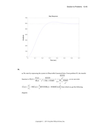
![12-46 Chapter 12: Design via State Space
By direct inspection we can write
&
1⎤ ⎡ x0 ⎤ ⎡ 0 ⎤
⎡ x0 ⎤ ⎡ − 10
⎡ x0 ⎤
⎢ x ⎥ = ⎢− 41665 0⎥ ⎢ x ⎥ + ⎢83335⎥ E s and y = [1 0]⎢ x ⎥
⎦⎣ 1 ⎦ ⎣
⎦
⎣ &1 ⎦ ⎣
⎣ 1⎦
The characteristic equation for this system is
s 2 + 10s + 41665 = 0 with roots at
-5±j204.06. To make the observer 10 times faster its poles will be placed at -50±j2040.6
The desired characteristic equation is
s 2 + 100s + 4.167 × 10 6 = 0
The error equation is given by
1⎤
⎡ − (10 + l1 )
&
e X = ( A − LC)e x = ⎢
⎥e x which has a characteristic equation
⎣− (41665 + l 2 ) 0⎦
s 2 + (10 + l1 ) s + (41665 + l 2 ) = 0
By equation coefficients with the desired characteristic equation we obtain
l1 = 100 − 10 = 90 and l 2 = 4.167 × 10 6 − 41665 = 4125335
Copyright © 2011 by John Wiley & Sons, Inc.](https://image.slidesharecdn.com/solutionscontrolsystemsengineeringbynormannice6ed-130502172814-phpapp02-131105052456-phpapp01/85/Solutions-control-system-sengineering-by-normannice-6ed-130502172814-phpapp02-858-320.jpg)
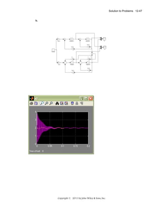
![12-48 Chapter 12: Design via State Space
39.
a. From the solution of Problem III the system can be written in phase variable form as:
0
1
0
⎡
⎤
⎡0 ⎤
⎥ ; B = ⎢0 ⎥ ;
Az = ⎢
0
0
1
z
⎢
⎥
⎢ ⎥
⎢− 0.000078 − 0.01265 − 0.5250⎥
⎢1⎥
⎣
⎦
⎣ ⎦
C z = [− 0.01197 × 10 −4
− 0.958 × 10 −4
0] ; D z = 0
The corresponding observability matrix is:
O Mz
⎡ Cz
⎢
= ⎢ Cz A z
⎢C z A 2
z
⎣
⎤ ⎡− 0.012 × 10 − 4
⎥ ⎢
0
⎥=⎢
⎥ ⎢ 0.0001 × 10 − 4
⎦ ⎣
− 0.958 × 10 − 4
− 0.019 × 10 − 4
0.0121 × 10 − 4
⎤
0
−4 ⎥
− 0.958 × 10 ⎥
0.491 × 10 − 4 ⎥
⎦
It is readily verified that the rank of O Mz is 3 and the system is observable.
Next we write the system in observable canonical form, for this let
− 0.958 × 10 −4 0.01197 × 10 −4
−
C ( s)
− 0.958 × 10 − 4 s − 0.01197 × 10 − 4
s2
s3
G ( s) =
= 3
=
0.525 0.01265 0.000078
R( s ) s + 0.525s 2 + 0.01265s + 0.000078
1+
+
+
s
s2
s3
From which we can write:
Copyright © 2011 by John Wiley & Sons, Inc.](https://image.slidesharecdn.com/solutionscontrolsystemsengineeringbynormannice6ed-130502172814-phpapp02-131105052456-phpapp01/85/Solutions-control-system-sengineering-by-normannice-6ed-130502172814-phpapp02-860-320.jpg)
![Solution to Problems 12-49
1⎛
1⎛
1
C ( s) = ⎜ − 0.525C ( s) + ⎜ − 0.958 × 10 − 4 R( s) − 0.01265C ( s ) + (− 0.01197 × 10 − 4 R( s ) − 0.000078C
⎜
s⎝
s⎝
s
Giving the following state flow diagram.
The system in observer canonical form is
0
⎡ − 0.5250 1 0⎤
⎡
⎤
⎢ − 0.01265 0 1⎥ ; B = ⎢ − 0.958 × 10 − 4 ⎥ ;
Ax = ⎢
x
⎥
⎢
⎥
⎢− 0.000078 0 0⎥
⎢− 0.01197 × 10 − 4 ⎥
⎣
⎦
⎣
⎦
C x = [1 0 0] ; D x = 0
And
⎡ − (0.5250 + l1 ) 1 0⎤
A x − L x C x = ⎢ − (0.01265 + l 2 ) 0 1⎥
⎢
⎥
⎢− (0.000078 + l 3 ) 0 0⎥
⎣
⎦
With a characteristic polynomial
s 3 + (0.525 + l1 ) s 2 + (0.01265 + l 2 ) + (0.000078 + l 3 ) = 0
Copyright © 2011 by John Wiley & Sons, Inc.](https://image.slidesharecdn.com/solutionscontrolsystemsengineeringbynormannice6ed-130502172814-phpapp02-131105052456-phpapp01/85/Solutions-control-system-sengineering-by-normannice-6ed-130502172814-phpapp02-861-320.jpg)
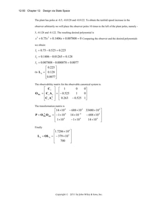
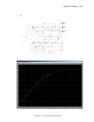
![Solution to Problems 12-55
&
⎡ x1 ⎤
⎡ x1 ⎤ ⎡0⎤
⎢ x ⎥ = ⎡ A − BK Bk e ⎤ ⎢ x ⎥ + ⎢0⎥ r
&
⎢ 2 ⎥ ⎢ −C
0 ⎥⎢ 2 ⎥ ⎢ ⎥
⎦ ⎢ ⎥ ⎢1 ⎥
⎢xN ⎥ ⎣
⎣& ⎦
⎣ xN ⎦ ⎣ ⎦
⎡ ⎡ 0 − 83.33⎤ ⎡166.67 ⎤
−
[k1
= ⎢ ⎢500
− 10 ⎥ ⎢ 0 ⎥
⎣
⎦ ⎣
⎦
⎢
[0 − 1]
⎢
⎣
⎡166.67 ⎤ ⎤ ⎡ x1 ⎤ ⎡0⎤
k2 ] ⎢
⎥ke ⎥⎢ ⎥ ⎢ ⎥
⎣ 0 ⎦ ⎥ ⎢ x 2 ⎥ + ⎢0 ⎥ r
0
⎥ ⎢ x N ⎥ ⎢1⎥
⎦⎣ ⎦ ⎣ ⎦
⎡− 166.67 k1 − (83.33 + 166.67 k 2 ) 166.67 k e ⎤ ⎡ x1 ⎤ ⎡0⎤
⎥ ⎢ x ⎥ + ⎢0 ⎥ r
0
= ⎢ 500
− 10
⎢
⎥⎢ 2 ⎥ ⎢ ⎥
⎢
⎥ ⎢ x N ⎥ ⎢1⎥
0
0
−1
⎣
⎦⎣ ⎦ ⎣ ⎦
⎡ x1 ⎤
y = [C 0]⎢ x 2 ⎥
⎢ ⎥
⎢xN ⎥
⎣ ⎦
The characteristic equation for the system above is:
s + 166.67 k1 83.33 + 166.67k 2
det( sI − A aug ) =
s + 10
− 500
0
1
− 166.67k e
0
s
= s 3 + (10 + 166.67 k1 ) s 2 + (1666.7 k1 + 41665 + 83335k 2 ) s + 83335k e
The desired polynomial for Ts = 0.5 sec and %OS=20% with an extra far away pole is:
( s 2 + 16 s + 130.65)( s + 50) = s 3 + 66 s 2 + 930.6 s + 6532.5
Equating coefficients in both polynomials we have:
10 + 166.67 k1 = 66 ⇒ k1 = 0.336
1666.7 k1 + 41665 + 83335k 2 = 930.6 ⇒ k 2 = −0.4955
83335k e = 6532.5 ⇒ k e = 0.0783884
Copyright © 2011 by John Wiley & Sons, Inc.](https://image.slidesharecdn.com/solutionscontrolsystemsengineeringbynormannice6ed-130502172814-phpapp02-131105052456-phpapp01/85/Solutions-control-system-sengineering-by-normannice-6ed-130502172814-phpapp02-867-320.jpg)
![Solution to Problems 12-57
42.
a. Using the following signal-flow graph,
1
1
x3 20000
s
800
1
x2 1
s
s
x1
1
u
y
-800
-100
the plant is represented in state space with
⎡0
⎢
A = ⎢0
⎢0
⎣
⎤
⎡ 0 ⎤
⎢
⎥
⎥
−100 20000⎥ ; B = ⎢ 0 ⎥ ; and C = [1 0 0].
⎢800 ⎦
⎥
⎥
0
− 800 ⎦
⎣
1
0
Using Eq. (12.26),
CM
⎡ 0
0
1.6 E07 ⎤
⎢
⎥
= ⎢ 0 1.6 E07 −1.44 E10 ⎥
⎢800 − 6.4 E05 5.12E08 ⎦
⎥
⎣
The system is controllable since the determinant of CM = -2.04e17. Use Eqs. (4.39) and (4.42) to find
ζ = 0.5912 and ωn = 135.3283 respectively. Factoring the denominator of Eq. (4.22), the required
poles are -80 ± j109.15. Place the third pole 10 times farther at = 800. Multiplying the three closedloop pole terms yields the desired characteristic equation
s3 + 960s2 + 1.463E05s + 1.4651E07 = 0.
Since the plant's characteristic equation is s3 + 900s2 + 80000s, we write the plant in controller
canonical form as
A cc
⎡− 900 − 80000 0 ⎤
⎡1 ⎤
⎢
⎢ ⎥
⎥
0
0 ⎥ ; Bcc = ⎢0 ⎥ ; and Ccc = [0 0 1.6E07]
=⎢ 1
⎢ 0
⎢0 ⎦
⎥
1
0⎦
⎣
⎣ ⎥
The controllability matrix for controllable canonical form is
C Mcc
⎡1
⎢
= ⎢0
⎢0
⎣
−900
1
0
730000⎤
⎥
−900 ⎥
⎥
1 ⎦
Comparing the first row of Acc to the desired characteristic equation and using the results of Problem
5, k1 = -(900 - 960) = 60; k2 = -(80000 - 1.463E05) = 66300; and k3 = -(0 - 1.465E07) = 1.465E07.
Hence.
Kcc = [60 66300
1.465E07]
The transformation matrix is,
⎡ 0
1.6E07⎤
⎥
1. 6E07
0 ⎥
⎢
⎢800 8E04
⎥
0 ⎦
⎣
⎢
P = CMCMcc-1 = 0
150
Copyright © 2011 by John Wiley & Sons, Inc.](https://image.slidesharecdn.com/solutionscontrolsystemsengineeringbynormannice6ed-130502172814-phpapp02-131105052456-phpapp01/85/Solutions-control-system-sengineering-by-normannice-6ed-130502172814-phpapp02-869-320.jpg)
![12-58 Chapter 12: Design via State Space
Transforming back to the original system,
K = KccP-1 = [9.1569E-01 3.7696E-03 7.5E-02]
The controller compensated system is
⎡ 0
1
⎢
A - BK = ⎢ 0
− 100
⎢
⎣−732. 55 −3.0157
0 ⎤
⎡ 0 ⎤
⎢
⎥
⎥
20000⎥ ; B = ⎢ 0 ⎥ ; C = [1 0 0]
⎢
⎥
⎥
−860 ⎦
⎣800 ⎦
b. To evaluate the steady-state error, use Eq. (7.89) where
⎡ 0
1
⎢
A - BK = ⎢ 0
− 100
⎢
⎣−732. 55 −3.0157
0 ⎤
⎥
20000⎥
⎥
−860 ⎦
is the system matrix. Thus,
s I − A −B K
−1 =
s 2 + 960 s + 1.4631 ×10 5
− 14651040
s + 860
2 + 860 s
s
− 732.55 s − 73255
− 3.0157 s − 732.55
1
s 3 + 960 s 2 + 1.4631 ×10 5 s + 14651040
20000
20000 s
s 2 + 100 s
The steady-state error is given by
sR(s)[1 − C s I − A − B K
− 1 B ] as s->0
For a step input, R(s) = 1/s. Since
−1 B = 1−
1− C s I − A − B K
1
16000000
s 3 + 960 s 2 + 1.4631×10 5 s + 14651040
for a step input e(∞) = -0.092073. Using Eqs. 12.115, the system with integral control is:
0
AI =
1
0
0
0
− 100
20000
0
− 800 K 1
−1
− 800 K 2
0
− 800 K 3 − 800
0
800 K e
0
0
;BI = 0 ;
0
1
C I = 1, 0, 0, 0
Assume the following desired characteristic equation:
(s3 + 960s2 + 1.463E05s + 1.4651E07)(s + 1000) =
s 4 + 1960 s 3 + 1.1063×10 6 s 2 + 1.6096×10 8 s + 1.4651×10 10 = 0,
which is the desired characteristic equation from part (a) plus an additional pole at -1000. But the
integral controlled system characteristic equation is
|sI - AI| = s 4 + 100 8 K 3 + 9 s 3 + 80000 K 3 + 200 K 2 + 1 s 2 + 16000000 K 1 s + 16000000 K e
Equating coefficients to the desired characteristic equation
100 8 K 3 + 9 = 1960; 80000 K 3 + 200 K 2 + 1 = 1.1063 ×10 6 ; 16000000 K 1 = 1.6096 ×10 8 ;
16000000 K e = 1.4651×10 10
Solving for the controller gains: K e = 915.69; K 1 = 10.06 ; K 2 = 0.05752 ; and K 3 = 1.325 .
Copyright © 2011 by John Wiley & Sons, Inc.](https://image.slidesharecdn.com/solutionscontrolsystemsengineeringbynormannice6ed-130502172814-phpapp02-131105052456-phpapp01/85/Solutions-control-system-sengineering-by-normannice-6ed-130502172814-phpapp02-870-320.jpg)
![Solution to Problems 12-59
Substituting into AI yields the integral controlled system.
0
0
0
0
− 100
20000
0
− 8048.2
− 46.016
− 1860
7.3255 ×10 5
−1
AI =
1
0
0
0
0
; B I = 0 ; C I = 1, 0, 0, 0
0
1
Finding the characteristic equation as a check yields
s 4 + 1960 s 3 + 1.1063 ×10 6 s 2 + 1.6096 ×10 8 s + 1.4651 ×10 10
which checks with the desired characteristic equation. Now check the steady-state error using
Eq. (7.89) using the integral controlled system. We find the error is zero.
c.
Program:
'Controller Compensated'
A=[0 1 0;0 -100 20000;-732.55 -3.0157 -860];
B=[0;0;800];
C=[1 0 0];
D=0;
S=ss(A,B,C,D)
step(S)
title('Controller Compensated')
pause
'Integral Controller'
A=[0 1 0 0;0 -100 20000 0;-8048.2 -46.016 -1860 7.3255e05;-1 0 0 0];
B=[0;0;0;1];
C=[1 0 0 0];
D=0;
S=ss(A,B,C,D)
step(S)
title('Integral Controller')
Computer response:
ans =
Controller Compensated
a=
x1
x2
x3
x1
0
1
0
x2
0 -100 2e+004
x3 -732.5 -3.016 -860
b=
u1
x1 0
x2 0
x3 800
c=
x1 x2 x3
y1 1 0 0
Copyright © 2011 by John Wiley & Sons, Inc.](https://image.slidesharecdn.com/solutionscontrolsystemsengineeringbynormannice6ed-130502172814-phpapp02-131105052456-phpapp01/85/Solutions-control-system-sengineering-by-normannice-6ed-130502172814-phpapp02-871-320.jpg)

![12-62 Chapter 12: Design via State Space
43.
Program:
%Enter G(s)
numg=0.072*conv([1 23],[1 0.05 0.04]);
deng=conv([1 0.08 0.04],poly([0.7 -1.7]));
'G(s)'
G=tf(numg,deng)
'Plant Zeros'
plantzeros=roots(numg)
%Input transient response specifications
Po=input('Type %OS ');
Ts=input('Type settling time
');
%Determine pole location
z=(-log(Po/100))/(sqrt(pi^2+log(Po/100)^2));
wn=4/(z*Ts);
%wn=pi/(Tp*sqrt(1-z^2));
[num,den]=ord2(wn,z);
r=roots(den);
poles=[r(1) r(2) plantzeros(2) plantzeros(3)]
characteristiceqdesired=poly(poles)
%Find controller canonical form of state-space representation of G(s)
'Controller Canonical Form'
[Ac Bc Cc Dc]=tf2ss(numg,deng)
%Design controller gains
Kc=acker(Ac,Bc,poles)
Acnew=Ac-Bc*Kc
Bcnew=Bc
Ccnew=Cc
Dcnew=Dc
characteristiceqcontroller=poly(eig(Acnew))
%Transform to phase-variable form
P=[0 0 0 1;0 0 1 0;0 1 0 0;1 0 0 0];
'Phase-variable form'
Ap=inv(P)*Ac*P
Bp=inv(P)*Bc
Cp=Cc*P
Dp=Dc
Kp=acker(Ap,Bp,poles)
Apnew=Ap-Bp*Kp
Bpnew=Bp
Cpnew=Cp
Dpnew=Dp
characteristiceqphase=poly(eig(Apnew))
[numt,dent]=ss2tf(Apnew,Bpnew,Cpnew,Dpnew);
T=tf(numt,dent);
'T(s)'
T=minreal(T)
step(T)
'T(s)'
Tzpk=zpk(T)
'Poles of T(s)'
p=pole(T)
Computer response:
ans =
Copyright © 2011 by John Wiley & Sons, Inc.](https://image.slidesharecdn.com/solutionscontrolsystemsengineeringbynormannice6ed-130502172814-phpapp02-131105052456-phpapp01/85/Solutions-control-system-sengineering-by-normannice-6ed-130502172814-phpapp02-874-320.jpg)
![12-66 Chapter 12: Design via State Space
44.
Program:
%Enter G(s)
numg=0.072*conv([1 23],[1 0.05 0.04]);
deng=conv([1 0.08 0.04],poly([0.7 -1.7]));
'Uncompensated Plant Transfer Function'
'G(s)'
G=tf(numg,deng)
'Uncompensated Plant Zeros'
plantzeros=roots(numg)
%Input transient response specifications
Po=input('Type %OS ');
Ts=input('Type settling time
');
%Determine pole location
z=(-log(Po/100))/(sqrt(pi^2+log(Po/100)^2));
wn=4/(z*Ts);
%wn=pi/(Tp*sqrt(1-z^2));
[num,den]=ord2(wn,z);
r=roots(den);
'Desired Observer Poles'
poles=[r(1) r(2) plantzeros(2) plantzeros(3)]'
'Desired Characteristic Equation of Observer'
poly(poles)
%Find phase variable form of state-space representation of Estimated Plant
%Find controller canonical form
[Ac Bc Cc Dc]=tf2ss(numg,deng);
%Transform to phase-variable form of Uncompensated Plant
P=[0 0 0 1;0 0 1 0;0 1 0 0;1 0 0 0];
'Phase-variable form of Estimated Plant'
Ap=inv(P)*Ac*P
Copyright © 2011 by John Wiley & Sons, Inc.](https://image.slidesharecdn.com/solutionscontrolsystemsengineeringbynormannice6ed-130502172814-phpapp02-131105052456-phpapp01/85/Solutions-control-system-sengineering-by-normannice-6ed-130502172814-phpapp02-878-320.jpg)
![12-70 Chapter 12: Design via State Space
0
0
0
− 14.781
− 0.06624
AI =
1
0
0
− 21.272
− 0.08568
0
1
0
− 370.05
− 1.6596
0
0
1
− 39.05
− 0.072
0
0
0
2542.8
0
0
0
;BI = 0 ;
0
1
C I = 0.06624 , 0.08568 , 1.6596 , 0.072 , 0
Finding the characteristic equation as a check yields
s 5 + 39.05 s 4 + 553.13 s 3 + 4241.3 s 2 + 232.65 s + 168.43
which checks with the desired. Now check the steady-state error using Eq. (7.89) using the integral
controlled system. We find the error is zero.
b.
Program:
%Design with Integral Control
'State-Space Representation of System with Integral Control'
AI=[0 1 0 0 0;0 0 1 0 0;0 0 0 1 0;...
-14.781 -21.272 -370.05 -39.05 2542.8;...
-0.06624 -0.08568 -1.6596 -0.072 0]
BI=[0;0;0;0;1]
CI=[0.06624 0.08568 1.6596 0.072 0]
DI=0
%Convert to transfer function
[numt,dent]=ss2tf(AI,BI,CI,DI);
'Integral Control Transfer Function'
'T(s)'
T=tf(numt,dent)
'Integral Control Transfer Function Zeros'
roots(numt)
'Integral Control Transfer Function Poles'
roots(dent)
step(T)
title('Step Response with Integral Controller')
Computer response:
ans =
State-Space Representation of System with Integral Control
AI =
1.0e+003 *
0
0
0
-0.0148
-0.0001
0.0010
0
0
-0.0213
-0.0001
0
0.0010
0
-0.3700
-0.0017
0
0
0.0010
-0.0390
-0.0001
0
0
0
2.5428
0
BI =
0
0
0
0
1
Copyright © 2011 by John Wiley & Sons, Inc.](https://image.slidesharecdn.com/solutionscontrolsystemsengineeringbynormannice6ed-130502172814-phpapp02-131105052456-phpapp01/85/Solutions-control-system-sengineering-by-normannice-6ed-130502172814-phpapp02-882-320.jpg)
![12-72 Chapter 12: Design via State Space
46.
a. We start by verifying that the system is controllable. For a system of this order it is best
to use MATLAB or other computing tools:
>>A=[-5 0 0 0 0; 0 0 1 0 0; -10.5229 -1066.67 -3.38028 23.5107 0; 0 993.804 3.125 -23.5107 0; 0 0
0 10 -10];
>>B = [5;0;0;0;0];
>>C = [0 0 0 1.2331e5 0];
>>D=0;
>> rank(ctrb(A,B))
ans =
5
So the system is controllable.
We also use MATLAB to find the corresponding transfer function:
>> [n,d]=ss2tf(A,B,C,D)
n=
1.0e+010 *
0 0.000000000000000 0.000000000000000 -0.002027466873438 0.665044169115073 -6.447695003806981
Copyright © 2011 by John Wiley & Sons, Inc.](https://image.slidesharecdn.com/solutionscontrolsystemsengineeringbynormannice6ed-130502172814-phpapp02-131105052456-phpapp01/85/Solutions-control-system-sengineering-by-normannice-6ed-130502172814-phpapp02-884-320.jpg)
![Solution to Problems 12-73
d=
1.0e+004 *
0.000100000000000 0.004189098000000 0.152603651149600 1.914775683863999
7.933055056779999 8.565653331000014
We use this information to express the system in state variable form:
1
0
0
0 ⎤
⎡ 0
⎡0⎤
⎢ 0
⎥
⎢0⎥
0
1
0
0 ⎥
⎢
⎢ ⎥
x 'x = ⎢ 0
0
0
1
0 ⎥ x + ⎢0⎥ u
⎢
⎥
⎢ ⎥
0
0
0
1 ⎥
⎢ 0
⎢0⎥
⎢ −85650 −79330 −19150 −1526 −41.89 ⎥
⎢1 ⎥
⎣
⎦
⎣ ⎦
y = [ −64476950038.1 −6650441691.2 −20274668.73 0 0] xx
Now we find the desired characteristic polynomial using a dominant pole approximation.
Assuming a pair of complex conjugate dominant poles Ts =
4
ξωn
= 2s , or ξωn = 2 . The
ξ = 0.6 damping factor. Therefore the dominant
2
s + 2ξωn s + ωn = s 2 + 4 s + 11.11 . The must be a total of 5
10% OS requirement corresponds to a
2
poles can be included in a
poles so arbitrarily we will add three poles 10 times to the left of the dominant poles, namely
( s + 20)3 . Thus the desired polynomial is given by:
D( s ) = ( s 2 + 4 s + 11.11)( s + 20)3
= s 5 + 64s 4 + 1451.11s 3 + 13466.77 s 2 + 45335.47 s + 88903.11
Under state feedback, the phase variable system will become
=
0
1
0
0
0
⎡
⎤
⎡0⎤
⎢
⎥
⎢0⎥
0
0
1
0
0
⎢
⎥
⎢ ⎥
⎢
⎥ x + ⎢0⎥ u
0
0
0
1
0
⎢
⎥
⎢ ⎥
0
0
0
0
1
⎢
⎥
⎢0⎥
⎢ −(85650 + k1x ) −(79330 + k2 x ) −(19150 + k3 x ) −(1526 + k4 x ) −(41.89 + k5 x ) ⎥
⎢1 ⎥
⎣ ⎦
⎣
⎦
With a characteristic equation given by:
Copyright © 2011 by John Wiley & Sons, Inc.](https://image.slidesharecdn.com/solutionscontrolsystemsengineeringbynormannice6ed-130502172814-phpapp02-131105052456-phpapp01/85/Solutions-control-system-sengineering-by-normannice-6ed-130502172814-phpapp02-885-320.jpg)
![12-74 Chapter 12: Design via State Space
det( sI − ( Ax − Bx K x ))
= s 5 + (41.89 + k5 x ) s 4 + (1526 + k4 x ) s 3 + (19150 + k3 x ) s 2
+ (79330 + k2 x ) s + (85650 + k1x )
We now equate the coefficients of this equation with those of the desired polynomial to get:
K x = [k1x
k2 x
k3 x
k4 x
k5 x ] = [3253.11 −33994.53 −5683.28 −74.89 22.11]
This vector is now transformed to the original coordinate system using MATLAB:
>> Ax=[0 1 0 0 0; 0 0 1 0 0; 0 0 0 1 0; 0 0 0 0 1;-8.565653331000014e4 7.933055056779999E4 -1.914775683863999e4 -0.152603651149600E4 0.004189098000000E4];
>> Bx = [0;0;0;0;1];
>> P=ctrb(A,B)*inv(ctrb(Ax,Bx));
>>Kz=Kx*inv(P);
K = [4.422 110.04 16.93 −1.75 −0.14]
b. The simulation is performed with the following commands:
>>Af=(A‐B*Kz)
>>step(Af,B,C,D)
Copyright © 2011 by John Wiley & Sons, Inc.](https://image.slidesharecdn.com/solutionscontrolsystemsengineeringbynormannice6ed-130502172814-phpapp02-131105052456-phpapp01/85/Solutions-control-system-sengineering-by-normannice-6ed-130502172814-phpapp02-886-320.jpg)
![Solution to Problems 12-75
5
0
Step Response
x 10
-1
-2
Amplitude
-3
-4
-5
-6
System: sys
Settling Time (sec): 1.83
-7
-8
0
0.5
1
System: sys
Peak amplitude: -7.96e+005
Overshoot (%): 9.7
1.5
2
2.5
3
Time (sec)
47.
a.
The open-loop block diagram is
Y h-Y cat
Spring
displacement
Desired
force
1
Input
voltage
1
100
1000
Input
transducer
Actuator
Fup
0 . 7883 ( s + 53 . 85 )
Fout
82300
2
(s + 15 . 47 s + 9283 )( s + 8 . 119 s + 376 .3 )
2
Pantograph
dynamics
From Chapter 3, the state-space representation for [Yh(s) – Ycat(s)]/Fup(s) is
Copyright © 2011 by John Wiley & Sons, Inc.
Spring](https://image.slidesharecdn.com/solutionscontrolsystemsengineeringbynormannice6ed-130502172814-phpapp02-131105052456-phpapp01/85/Solutions-control-system-sengineering-by-normannice-6ed-130502172814-phpapp02-887-320.jpg)
![12-76 Chapter 12: Design via State Space
1
0
0 ⎤
⎡ 0
⎡ 0 ⎤
⎢ -9353 -14.286 769.23 14.286 ⎥
⎢ 0 ⎥
⎥x+⎢
⎥f
&
x=⎢
⎢ 0
⎢ 0 ⎥ up
0
0
1 ⎥
⎢
⎥
⎢
⎥
⎣ 406.98 7.5581 -406.98 -9.3023⎦
⎣ 0.0581⎦
y = [0.94911 0 0
0]x
⎡y h ⎤
.
⎢y h ⎥
where y = yh - ycat and x = ⎢ ⎥
yf
⎢. ⎥
⎣y f ⎦
Let vi represent the input voltage shown on the diagram. Thus, fup = vi/1000.
Also, fout = 82300(yh - ycat).
Thus, fout = 82300y
Substituting fup and fout into the state-equations above yields
1
0
0 ⎤
0
⎡ 0
⎡
⎤
⎢ -9353 -14.286 769.23 14.286 ⎥
⎢
⎥
0
⎥x+⎢
⎥ vi
&
x=⎢
⎢ 0
⎢
⎥
0
0
1 ⎥
0
⎢
⎥
⎢
-3 ⎥
⎣ 406.98 7.5581 -406.98 -9.3023⎦
⎣ 0.0581x10 ⎦
fout = [78,112 0 0 0]x
Thus,
1
0
0 ⎤
⎡ 0
⎢ -9353 -14.286 769.23 14.286 ⎥
A=⎢
0
0
0
1 ⎥
⎢ 406.98 7.5581 -406.98 -9.3023⎦
⎥
⎣
0
⎡
⎤
⎥
0
⎢
B=⎢
⎥
0
⎢ 0.0581x10⁻³ ⎦
⎥
⎣
K = [k1
k2
k3
k4 ]
Hence,
A-BK =
[0 , 1 , 0 , 0
Copyright © 2011 by John Wiley & Sons, Inc.](https://image.slidesharecdn.com/solutionscontrolsystemsengineeringbynormannice6ed-130502172814-phpapp02-131105052456-phpapp01/85/Solutions-control-system-sengineering-by-normannice-6ed-130502172814-phpapp02-888-320.jpg)
![Solution to Problems 12-77
[-9350 , -14.3 , 769 , 14.3
[0 , 0 , 0 , 1
[407 - 0.0000581 k1 , 7.56 - .0000581 k2 , -407 - 0.0000581 k3 , -9.30 - 0.0000581 k4]
and
| A-BK| = s4 + (0.0000581 k4 + 23.60) s3
+ (0.00083083 k4 + 0.00083083 k2 + 9781.882 + 0.0000581 k3) s2
+ (0.00083083 k1 + 81141.36 + 0.543235 k4 + 0.00083083 k3 + 0.0446789 k2) s
+(0 .0446789 k1 +0.3492467 107 + 0.543235 k3)
Input transient response specifications,
Po = 20
Ts = 1
yields poles at
-4.0000 + 7.8079i, -4.0000 - 7.8079i, -53.8500, -50.0000
Thus, the desired characteristic equation is
s4 + 112s3 + 3600s2 + 29500s + 207000 = 0
We now equate the coefficients of |A-BK| to the coefficients of the desired characteristic equation.
For compactness we solve for the coefficients, K, using the form FK = G, where
F=
0
0
0.00083083
0 .0446789
0
0.00083083
0.0446789
0
0
0.0000581
0.0000581
0.00083083
0.00083083
0.543235
0.543235
0
and
G=
88.4
–6181.882
-51641.36
-3285467
Solving for K using K = F-1G
K=
-4.8225e8
-0.1131e8
0.3361e8
0.0152e8
b.
Integral Control Design
A=
1.0e+03 *
0
-9.3530
0
0.4070
B=
0.0010
-0.0143
0
0.0076
0
0.7692
0
-0.4070
0
0.0143
0.0010
-0.0093
Copyright © 2011 by John Wiley & Sons, Inc.](https://image.slidesharecdn.com/solutionscontrolsystemsengineeringbynormannice6ed-130502172814-phpapp02-131105052456-phpapp01/85/Solutions-control-system-sengineering-by-normannice-6ed-130502172814-phpapp02-889-320.jpg)
![12-78 Chapter 12: Design via State Space
1.0e-04 *
0
0
0
0.5810
C=
78112
0
0
0
Aaug = A-BK =
[0 , 1. , 0 , 0 , 0
[-9350. , -14.3 , 769. , 14.3 , 0
[0 , 0 , 0 , 1. , 0
[407. - 0.0000581 k1 , 7.56 - 0.0000581 k2 , -407. - 0.0000581 k3 ,
-9.30 - 0.0000581 k4 , 0.0000581 Ke
[-78100. , 0 , 0 , 0 , 0]
Desired poles
Po = 20
Ts = 1
Determine pole location
poles = -4.0000 + 7.8079i, -4.0000 - 7.8079i, -53.85, -50 , -50
Desired characteristic equation
s5 + 162s4 + 0.919e4s3 + 0.210e6s2 + 0.168e7s + 0.104e8
System characteristic equation
|sI-Aaug| =
s5 + (23.60 + 0.0000581 k4) s4
+ (0.00083083 k4 + 0.00083083 k2 + 0.0000581 k3 + 9781.882) s3
+ (0.00083083 k1 + 81141.36 + 0.0446789 k2 + 0.543235 k4 + 0.00083083 k3) s2
+ (0.0446789 k1 + 64.887823 Ke + 0.543235 k3 + 0.3492467 107 ) s
+ 3489.42209 Ke
Solving for Coefficients, K, using FK = G as in (a), where
F
0
0
0
8.3083e-04
8.3083e-04 4.4679e-02
4.4679e-02
0
0
0
G=
1.3840e+02
-5.9188e+02
1.2886e+05
-1.8125e+06
1.0800e+07
0
5.8100e-05
8.3083e-04
5.4324e-01
0
5.8100e-05
0
8.3083e-04
0
5.4324e-01
0
0
6.4888e+01
0
3.4894e+03
Copyright © 2011 by John Wiley & Sons, Inc.](https://image.slidesharecdn.com/solutionscontrolsystemsengineeringbynormannice6ed-130502172814-phpapp02-131105052456-phpapp01/85/Solutions-control-system-sengineering-by-normannice-6ed-130502172814-phpapp02-890-320.jpg)
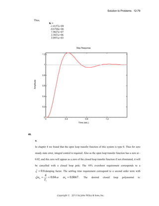
![12-80 Chapter 12: Design via State Space
( s 2 + 0.08s + 0.0044)( s + 0.02)( s + 0.5) = s 4 + 0.6s 3 + 0.056s 2 + 0.003088s + 0.000044
where a far away pole was arbitrarily added at -0.5.
Following equation (12.115a) in the text, the closed loop system matrix A is given by
⎡ A − BK Bk e ⎤
A CL = ⎢
0 ⎥
⎣ −C
⎦
⎡ ⎡− 0.04167
− 0.0058⎤ ⎡ 5.2 ⎤
0
⎡ 5.2 ⎤ ⎤
⎢⎢
⎥ − ⎢− 5.2⎥[k k k ] ⎢− 5.2⎥ k ⎥
− 0.24 0.0058 ⎥ ⎢
0.0217
2
3
⎥ 1
⎢
⎥ e⎥
= ⎢⎢
⎢⎢
⎢ 0 ⎥ ⎥
− 2.4 ⎥ ⎢ 0 ⎥
0
100
⎣
⎦ ⎣
⎦
⎣
⎦
⎢
⎥
0
[0 0 − 1]
⎣
⎦
− 5.2k 2
− (0.0058 + 5.2k 3 ) 5.2k e ⎤
⎡− (0.04167 + 5.2k1 )
⎢ 0.0217 + 5.2k
− 0.24 + 5.2k 2
0.0058 + 5.2k 3
− 5.2k e ⎥
1
⎢
⎥
=
⎢
0
100
− 2.4
0 ⎥
⎢
⎥
0
0
−1
0 ⎦
⎣
The corresponding characteristic polynomial is:
s 4 + (2.68167 + 5.2k1 − 5.2k 2 ) s 3 + (0.1060088 + 13.728k1 − 12.583844k 2 − 520k 3 ) s 2 +
(0.01241932 + 2.9952k1 − 0.2492256k 2 − 10.3844k 3 − 520k e ) s − 10.3844k e
Equating the coefficients of this polynomial with those of the desired polynomial and solving
simultaneous equations one gets
K = [k1
k2
k 3 ] = [− 0.004174 0.39615 − 0.0096] and k e = −4.237125 × 10 −6
Copyright © 2011 by John Wiley & Sons, Inc.](https://image.slidesharecdn.com/solutionscontrolsystemsengineeringbynormannice6ed-130502172814-phpapp02-131105052456-phpapp01/85/Solutions-control-system-sengineering-by-normannice-6ed-130502172814-phpapp02-892-320.jpg)
![12-82 Chapter 12: Design via State Space
49.
We’ll start by finding the key parameters needed to meet specifications:
•
The damping ratio, ζ, for a 4.32% overshoot is:
− ln(%OS / 100)
ζ =
•
π 2 + ln 2 (%OS / 100)
=
− ln(4.32 / 100)
π 2 + ln 2 (4.32 / 100)
= 0.707
The natural frequency, ωn, for a settling time = 4 sec at the above ζ is:
Ts =
4
ζω n
⇒4=
4
⇒ ω n = 1.414 rad/sec
0.707ω n
•
The coordinates of the required dominant poles, – ζωn ± jωd = – 1 ± j 1.
•
The open-loop transfer-function of the “plant” is given by equation (3.73):
G ( s) =
Y (s)
= C(sI − A) -1 B + D
U (s)
Here:
− 40 ⎤ ⎡ s + 20
40
⎤
⎡ s 0⎤ ⎡ − 20
(sI − A ) = ⎢
⎥ − ⎢0.2491 − 0.0191⎥ = ⎢− 0.2491 s + 0.0191⎥
⎦
⎦ ⎣
⎣0 s ⎦ ⎣
40
⎡ s + 0.0191 0.2491⎤
⎡ s + 20
⎤
adj ⎢
⎢
⎥
s + 20 ⎥
adj(sI − A )
⎦
⎣− 0.2491 s + 0.0191⎦ = ⎣ − 40
(sI − A ) -1 =
=
det (sI − A )
s 2 + 20.0191s + 10.346
s 2 + 20.0191s + 10.346
Hence:
G (s) =
Y (s)
=
U (s)
[0
⎡ s + 0.0191 0.2491⎤ ⎡ 0 ⎤
0.06154] ⎢
s + 20 ⎥ ⎢1000⎥
61.54 (s + 20)
⎣ − 40
⎦⎣
⎦=
2
2
s + 20.0191s + 10.346
s + 20.0191s + 10.346
Now, we write the closed-loop state equations for the system with integral control in a form similar
to that given in the text by equations 12.115a and 12.115b (Figure 12.21):
Copyright © 2011 by John Wiley & Sons, Inc.](https://image.slidesharecdn.com/solutionscontrolsystemsengineeringbynormannice6ed-130502172814-phpapp02-131105052456-phpapp01/85/Solutions-control-system-sengineering-by-normannice-6ed-130502172814-phpapp02-894-320.jpg)
![Solution to Problems 12-83
&
⎡ Ia ⎤ ⎡
0 ⎤ ⎡ I a ⎤ ⎡0 ⎤
− 20
− 40
⎢ ⎥ ⎢
⎥⎢ ⎥ ⎢ ⎥
&
⎢ ω ⎥ = ⎢0.2491 − 1000k1 − 0.0191 − 1000k 2 1000 K e ⎥ ⎢ ω ⎥ + ⎢0⎥ r
⎢xN ⎥ ⎢
0
0 ⎥ ⎢ x N ⎥ ⎢1⎥
− 0.06154
⎦⎣ ⎦ ⎣ ⎦
⎣& ⎦ ⎣
⎡ Ia ⎤
And the output equation is given by: y (t ) = v (t ) = [0 0.06154 0] ⎢ ω ⎥
⎢ ⎥
⎢xN ⎥
⎣ ⎦
− 20
⎡ s 0 0⎤ ⎡
⎢0 s 0⎥ − ⎢0.2491 − 1000 K
(sI − A ) = ⎢
1
⎥ ⎢
⎢0 0 s ⎥ ⎢
0
⎦ ⎣
⎣
s + 20
⎡
⎢− 0.2491 + 1000 K
1
⎢
⎢
0
⎣
− 40
0 ⎤
− 0.0191 − 1000 K 2 1000 K e ⎥ =
⎥
⎥
− 0.06154
0 ⎦
40
s + 0.0191 + 1000 K 2
0.06154
⎤
− 1000 K e ⎥
⎥
⎥
s
⎦
0
The characteristic polynomial for that system is:
s 3 + ( 20.0191 + 1000 K 2 ) s 2 + (−40000 K1 + 20000 K 2 + 61.54 K e + 10.346) s + 1230.8 K e
The desired characteristic polynomial (with the third pole placed to cancel the zero at -20) is:
s 3 + 22 s 2 + 42 s + 40
Equating coefficients of the characteristic polynomials yields:
K1 = 0.000249, K2 = 0.001981, Ke = 0.0325.
Substituting these values into the state equations for the system yields:
&
⎡ I a ⎤ ⎡ − 20
− 40
0 ⎤ ⎡ I a ⎤ ⎡0 ⎤
⎢ ⎥ ⎢
&
−2
32.5⎥ ⎢ ω ⎥ + ⎢0⎥ r
⎢ ω ⎥ = ⎢0.0001
⎥⎢ ⎥ ⎢ ⎥
⎢ xN ⎥ ⎢ 0
& ⎦ ⎣
− 0.06154
0 ⎥ ⎢ x N ⎥ ⎢1⎥
⎦⎣ ⎦ ⎣ ⎦
⎣
Copyright © 2011 by John Wiley & Sons, Inc.](https://image.slidesharecdn.com/solutionscontrolsystemsengineeringbynormannice6ed-130502172814-phpapp02-131105052456-phpapp01/85/Solutions-control-system-sengineering-by-normannice-6ed-130502172814-phpapp02-895-320.jpg)
![12-84 Chapter 12: Design via State Space
⎡ Ia ⎤
y (t ) = v (t ) = [0 0.06154 0] ⎢ ω ⎥
⎢ ⎥
⎢xN ⎥
⎣ ⎦
To check our assumptions, we use Eq. (3.73) and MATLAB to find the closed-loop transfer function
of the system to be:
T ( s) =
2s + 40
2( s + 20)
2
Y (s)
= 2
= 3
= 2
2
R( s) s + 22 s + 42s + 40 ( s + 2 s + 2)( s + 20) s + 2s + 2
The following MATLAB file was written to plot the step response.
A=[-20 -40 0; 0.0001 -2.000 32.5; 0
-0.06154 0];
B= [0; 0; 1];
C = [ 0
0.06154 0];
D = 0;
[num, den]= ss2tf(A,B,C,D,1);
T = tf(num, den);
%T is the closed-loop TF
step (T);
The characteristics displayed on the step response shown below indicate that the desired transient and
steady-state response requirements are met.
To find, analytically, the steady-state error for a unit step input, we apply Equation (7.96) to the state
equations to obtain:
− 40
0 ⎤
⎡ − 20
⎢0.0001
−2
e(∞) = 1 + [0 0.06154 0] ⎢
32.5⎥
⎥
⎢ 0
− 0.06154
0 ⎥
⎣
⎦
Copyright © 2011 by John Wiley & Sons, Inc.
−1
⎡0 ⎤
⎢0 ⎥ = 0
⎢ ⎥
⎢1⎥
⎣ ⎦](https://image.slidesharecdn.com/solutionscontrolsystemsengineeringbynormannice6ed-130502172814-phpapp02-131105052456-phpapp01/85/Solutions-control-system-sengineering-by-normannice-6ed-130502172814-phpapp02-896-320.jpg)

![13-2 Chapter 13: Digital Control Systems
We find that the root locus crosses at approximately 0.93 ± j0.11 with 7.659x10⁻⁴K = 8.63x10⁻³.
Hence, K = 11.268.
c.
1
(7.659x10⁻⁴ K)(1.95696)
lim(z − 1)Ge (z) =
= 0.1366;
0.12366
T z →1
1
= 7.321
e(∞) =
Kv
Kv =
d.
Program:
T=0.1;
numf=0.16;
denf=[1 1.32 0 0];
'F(s)'
F=tf(numf,denf)
numc=conv([1 0],numf);
denc=denf;
%Input sampling time
%Numerator of F(s)
%Denominator of F(s)
%Display label
%Display F(s)
%Differentiate F(s) to compensate
%for c2dm which assumes series zoh
%Denominator of continuous system
%same as denominator of F(s)
%Form continuous system, C(s)
%Cancel common poles and zeros
%Convert to z assuming zoh
C=tf(numc,denc);
C=minreal(C,1e-10);
D=c2d(C,T,'zoh');
'F(z)'
D=minreal(D,1e-10)
%Cancel common poles and zeros and display
rlocus(D)
pos=(16.3);
z=-log(pos/100)/sqrt(pi^2+[log(pos/100)]^2);
zgrid(z,0)
title(['Root Locus with ' , num2str(pos), ' Percent Overshoot Line'])
[K,p]=rlocfind(D)
%Allows input by selecting point on
%graphic
Computer response:
ans =
F(s)
Transfer function:
0.16
-------------s^3 + 1.32 s^2
ans =
F(z)
Transfer function:
0.0007659 z + 0.000733
---------------------z^2 - 1.876 z + 0.8763
Sampling time: 0.1
Select a point in the graphics window
selected_point =
9.2969e-001 +1.0219e-001i
K =
9.8808e+000
Copyright © 2011 by John Wiley & Sons, Inc.](https://image.slidesharecdn.com/solutionscontrolsystemsengineeringbynormannice6ed-130502172814-phpapp02-131105052456-phpapp01/85/Solutions-control-system-sengineering-by-normannice-6ed-130502172814-phpapp02-899-320.jpg)
![13-4 Chapter 13: Digital Control Systems
Gc (s) =
94.87(s + 1.32)
. Using a sampling interval of 0.01 s, the Tustin transformation of Gc(s)
(s + 4.606)
is Gc (z) =
93.35(z − 0.9869) 93.35z − 92.12
=
.
(z − 0.955)
z − 0.955
b. Cross multiplying,
(z - 0.955)X(z) = (93.35z – 92.12)E(z)
Solving for the highest power of z operating on X(z),
zX(z) = (93.35z – 92.12)E(z) + 0.955X(z)
Solving for X(z),
X(z) = (93.35 – 92.12z-1)E(z) + 0.955z-1X(z)
Implementing this equation as a flowchart yields the following diagram
c.
Program:
's-plane lead design for Challenge - Lead Comp'
clf
%Clear graph on screen.
'Uncompensated System'
%Display label.
numg=0.16;
%Generate numerator of G(s).
deng=poly([0 -1.32]);
%Generate denominator of G(s).
'G(s)'
%Display label.
G=tf(numg,deng);
%Create G(s).
Gzpk=zpk(G)
%Display G(s).
pos=input('Type desired percent overshoot ');
%Input desired percent overshoot.
z=-log(pos/100)/sqrt(pi^2+[log(pos/100)]^2);
%Calculate damping ratio.
Tp=input('Type Desired Peak Time ');
%Input desired peak time.
wn=pi/(Tp*sqrt(1-z^2));
%Evaluate desired natural frequency.
b=input('Type Lead Compensator Zero, (s+b). b= ');
%Input lead compensator zero.
done=1;
%Set loop flag.
while done==1
%Start loop for trying lead
%compensator pole.
a=input('Enter a Test Lead Compensator Pole, (s+a). a =
');
%Enter test lead compensator pole.
numge=conv(numg,[1 b]);
%Generate numerator of Gc(s)G(s).
denge=conv([1 a],deng);
%Generate denominator of Gc(s)G(s).
Ge=tf(numge,denge);
%Create Ge(s)=Gc(s)G(s).
clf
%Clear graph on screen.
Copyright © 2011 by John Wiley & Sons, Inc.](https://image.slidesharecdn.com/solutionscontrolsystemsengineeringbynormannice6ed-130502172814-phpapp02-131105052456-phpapp01/85/Solutions-control-system-sengineering-by-normannice-6ed-130502172814-phpapp02-901-320.jpg)
![Solutions to Case Studies Challenges 13-5
rlocus(Ge)
%Plot compensated root locus with
%test lead compensator pole.
axis([-5 2 -8 8]);
%Change axes ranges.
sgrid(z,wn)
%Overlay grid on lead-compensated
%root locus.
title(['Lead-Compensated Root Locus with ' , num2str(pos),...
'% Overshoot Line, Lead Pole at ', num2str(-a),...
' and Required Wn'])
%Add title to lead-compensated root
%locus.
done=input('Are you done? (y=0,n=1) ');
%Set loop flag.
end
%End loop for trying compensator
%pole.
[K,p]=rlocfind(Ge);
%Generate gain, K, and closed-loop
%poles, p, for point selected
%interactively on the root locus.
'Gc(s)'
%Display label.
Gc=K*tf([1 b],[1 a])
%Display lead compensator.
'Gc(s)G(s)'
%Display label.
Ge
%Display Gc(s)G(s).
'Closed-loop poles = '
%Display label.
p
%Display lead-compensated system's
%closed-loop poles.
f=input('Give pole number that is operating point
');
%Choose lead-compensated system
%dominant pole.
'Summary of estimated specifications for selected point on lead'
'compensated root locus'
%Display label.
operatingpoint=p(f)
%Display lead-compensated dominant
%pole.
gain=K
%Display lead-compensated gain.
estimated_settling_time=4/abs(real(p(f)))
%Display lead-compensated settling
%time.
estimated_peak_time=pi/abs(imag(p(f)))
%Display lead-compensated peak time.
estimated_percent_overshoot=pos %Display lead-compensated percent
%overshoot.
estimated_damping_ratio=z
%Display lead-compensated damping
%ratio.
estimated_natural_frequency=sqrt(real(p(f))^2+imag(p(f))^2)
%Display lead-compensated natural
%frequency.
s=tf([1 0],1);
%Create transfer function, "s".
sGe=s*Ge;
%Create sGe(s) to evaluate Kv.
sGe=minreal(sGe);
%Cancel common poles and zeros.
Kv=dcgain(K*sGe)
%Display lead-compensated Kv.
ess=1/Kv
%Display lead-compensated steady%state error for unit ramp input.
'T(s)'
%Display label.
T=feedback(K*Ge,1)
%Create and display lead-compensated
%T(s).
'Press any key to continue and obtain the lead-compensated step'
'response'
%Display label
pause
step(T)
%Plot step response for lead
%compensated system.
title(['Lead-Compensated System with ' ,num2str(pos),'% Overshoot'])
%Add title to step response of PD
%compensated system.
pause
'z-plane conversion for Challenge - Lead Comp'
clf
%Clear graph.
'Gc(s) in polynomial form'
%Print label.
Gcs=Gc
%Create Gc(s) in polynomial form.
'Gc(s) in polynomial form'
%Print label.
Copyright © 2011 by John Wiley & Sons, Inc.](https://image.slidesharecdn.com/solutionscontrolsystemsengineeringbynormannice6ed-130502172814-phpapp02-131105052456-phpapp01/85/Solutions-control-system-sengineering-by-normannice-6ed-130502172814-phpapp02-902-320.jpg)
![13-6 Chapter 13: Digital Control Systems
Gcszpk=zpk(Gcs)
%Create Gc(s) in factored form.
'Gc(z) in polynomial form via Tustin Transformation'
%Print label.
Gcz=c2d(Gcs,1/100,'tustin')
%Form Gc(z) via Tustin
%transformation.
'Gc(z) in factored form via Tustin Transformation'
%Print label.
Gczzpk=zpk(Gcz)
%Show Gc(z) in factored form.
'Gp(s) in polynomial form'
%Print label.
Gps=G
%Create Gp(s) in polynomial form.
'Gp(s) in factored form'
%Print label.
Gpszpk=zpk(Gps)
%Create Gp(s) in factored form.
'Gp(z) in polynomial form'
%Print label.
Gpz=c2d(Gps,1/100,'zoh')
%Form Gp(z) via zoh transformation.
'Gp(z) in factored form'
%Print label.
Gpzzpk=zpk(Gpz)
%Form Gp(z) in factored form.
pole(Gpz)
%Find poles.
Gez=Gcz*Gpz;
%Form Ge(z) = Gc(z)Gp(z).
'Ge(z) = Gc(z)Gp(z) in factored form'
%Print label.
Gezzpk=zpk(Gez)
%Form Ge(z) in factored form.
'z-1'
%Print label.
zm1=tf([1 -1],1,1/100)
%Form z-1.
zm1Gez=minreal(zm1*Gez,.00001);
'(z-1)Ge(z)'
%Print label.
zm1Gezzpk=zpk(zm1Gez)
pole(zm1Gez)
Kv=300*dcgain(zm1Gez)
Tz=feedback(Gez,1)
step(Tz)
title('Closed-Loop Digital Step Response')
%Add title to step response.
Computer response:
ans =
s-plane lead design for Challenge - Lead Comp
ans =
Uncompensated System
ans =
G(s)
Zero/pole/gain:
0.16
---------s (s+1.32)
Type desired percent overshoot 10
Type Desired Peak Time 1
Type Lead Compensator Zero, (s+b). b= 1.32
Enter a Test Lead Compensator Pole, (s+a). a =
Are you done? (y=0,n=1) 0
Select a point in the graphics window
selected_point =
-2.3045 + 3.1056i
ans =
Copyright © 2011 by John Wiley & Sons, Inc.
4.606](https://image.slidesharecdn.com/solutionscontrolsystemsengineeringbynormannice6ed-130502172814-phpapp02-131105052456-phpapp01/85/Solutions-control-system-sengineering-by-normannice-6ed-130502172814-phpapp02-903-320.jpg)
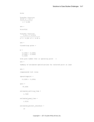
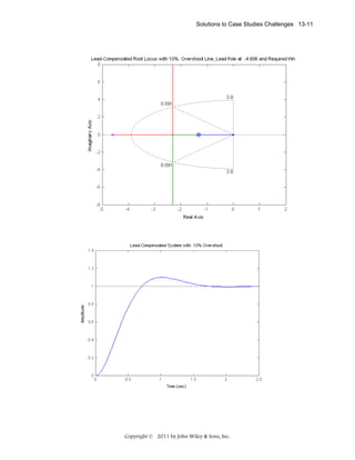
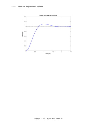

![Solutions to Problems 13-15
T 2 [z −1 e −aT + z −2 e −2aT ] T 2 ze −aT [z + e − aT ]
=
−3
−aT 3
− aT 3
z (z − e )
(z − e )
∞
d. f(t) = cos(ωkT); f*(t) =
∑ cos(ωkT)δ (t
− kT) ; F*(s) =
∞
∑ cos(ωkT)e
− kTs
k =0
k =0
(e jωkT + e − jωkT )e −kTs 1 ∞ T (s − jω ) − k
T (s + jω ) − k
= ∑ (e
) +(e
)
∑
2
2 k=0
k =0
∞
=
But,
∞
∑ x-k
k=0
=
1
.
1 - x-1
Thus,
F*(s) =
=
2 − e −Ts ( e jωT + e− jωT )
⎤
1⎡
1
1
⎤ 1⎡
+
=
−T (s − jω )
−T (s + jω )
⎢ 1− e −T (s − jω ) − e −T (s + jω ) ) + e −T (s− jω )e − T (s + jω ) ⎥
⎦ 2⎣
1−e
2 ⎣ 1− e
⎦
1 − z −1 cos(ωT )
1⎡
2 − e − Ts (2cos(ωT )
⎤
=
2 ⎢ 1− e −Ts (e jωT + e − jωT ) + e −2Ts ⎥ 1 − 2z−1 cos(ωT ) + z −2
⎣
⎦
Therefore,
F(z) =
z(z − cos(ω T))
z − 2z cos(ωT ) + 1
2
2.
Program:
syms T a w n
'(a)'
'f(kT)'
f=exp(-a*n*T);
pretty(f)
'F(z)'
F=ztrans(f);
pretty(F)
%Construct symbolic objects for
%'T', 'a','w', and 'n'.
%Display label.
%Display label.
%Define f(kT).
%Pretty print f(kT)
%Display label.
%Find z-transform, F(z).
%Pretty print F(z).
'(b)'
'f(kT)'
f=exp(-0*n*T);
pretty(f)
'F(z)'
F=ztrans(f);
pretty(F)
%Display label.
%Display label.
%Define f(kT)
%Pretty print f(kT)
%Display label.
%Find z-transform, F(z).
%Pretty print F(z).
'(c)'
'f(kT)'
f=(n*T)^2*exp(-a*n*T);
pretty(f)
'F(z)'
F=ztrans(f);
pretty(F)
%Display label.
%Display label.
%Define f(kT)
%Pretty print f(kT)
%Display label.
%Find z-transform, F(z).
%Pretty print F(z).
'(d)'
'f(kT)'
f=cos(w*n*T);
pretty(f)
'F(z)'
%Display label.
%Display label.
%Define f(kT)
%Pretty print f(kT)
%Display label.
Copyright © 2011 by John Wiley & Sons, Inc.](https://image.slidesharecdn.com/solutionscontrolsystemsengineeringbynormannice6ed-130502172814-phpapp02-131105052456-phpapp01/85/Solutions-control-system-sengineering-by-normannice-6ed-130502172814-phpapp02-912-320.jpg)
 + 4.965 .9000
- 7.875 .5000
+ 4.688 .1000
ans =
(c)
(z + 1.) (z + .3000) (z + .4000)
------------------------------------z (z - .2000) (z - .5000) (z - .7000)
n
n
-1.714 charfcn[1](n) - 26.16 charfcn[0](n) + 38.16 .7000 - 72.00 .5000
n
+ 60.00 .2000
5.
a.
By division
Instant
0
1
2
3
4
5
6
7
8
9
10
11
12
13
14
15
16
17
18
19
20
21
22
23
24
25
26
27
28
29
30
By Formula
Value
k
1
9.8
31.6
46.88
53.4016
53.43488
49.64608
44.043776
37.90637056
31.95798733
26.5581568
21.84639857
17.83896791
14.48905384
11.72227881
9.456567702
7.612550239
6.118437551
4.911796342
3.939668009
3.15787423
2.529983782
2.026197867
1.622284879
1.298623886
1.039376712
0.831787937
0.665602292
0.532584999
0.4261299
0.34094106
Copyright © 2011 by John Wiley & Sons, Inc.
Value
0
1
2
3
4
5
6
7
8
9
10
11
12
13
14
15
16
17
18
19
20
21
22
23
24
25
26
27
28
29
30
1
9.8
31.6
46.88
53.4016
53.43488
49.64608
44.043776
37.90637056
31.95798733
26.5581568
21.84639857
17.83896791
14.48905384
11.72227881
9.456567702
7.612550239
6.118437551
4.911796342
3.939668009
3.15787423
2.529983782
2.026197867
1.622284879
1.298623886
1.039376712
0.831787937
0.665602292
0.532584999
0.4261299
0.34094106](https://image.slidesharecdn.com/solutionscontrolsystemsengineeringbynormannice6ed-130502172814-phpapp02-131105052456-phpapp01/85/Solutions-control-system-sengineering-by-normannice-6ed-130502172814-phpapp02-916-320.jpg)

![Solutions to Problems 13-31
=
(T 2 − 2e −T + 2 − 2T ) z 2 + (4e −T − 4 + 2Te −T + 2T + T 2 − T 2 e −T ) z + (2 − 2e−T − 2Te −T − T 2 e −T )
( z − 1) 2 ( z − e −T )
G2 ( s ) = (1 − e − sT )
1
s ( s + 1)
3
transforms into
1
H 2 ( z)
2
Thus, the closed-loop transfer function is
⎡
⎤
1
T ( z ) = G1 ( z )G2 ( z ) ⎢
⎥
⎣ 1 + H1 ( z ) + H 2 ( z ) ⎦
12.
z-1
G(z) = z
z ⎧s2(s1+ 1)⎫ .
⎨
⎬
⎩
⎭
Using Eq. (13.49)
(1 - e-T)
(T-1+e-T)z + (1-e-T-Te-T)
T
G(z) = z - 1 -T =
z-e
(z-1)(z-e-T)
But,
G(z)
(T-1+e-T) z + (1-e-T-Te-T)
T(z) = 1 + G(z) = 2
z + (T-2) z + (1-Te-T)
The roots of the denominator are inside the unit circle for 0<T<3.923.
13.
Program:
numg1=10*[1 7];
deng1=poly([-1 -3 -4 -5]);
G1=tf(numg1,deng1);
for T=5:-.01:0;
Gz=c2d(G1,T,'zoh');
Tz=feedback(Gz,1);
r=pole(Tz);
rm=max(abs(r));
if rm<=1;
break;
end;
end;
T
r
rm
Computer response:
T =
3.3600
r =
-0.9990
-0.0461
-0.0001
Copyright © 2011 by John Wiley & Sons, Inc.](https://image.slidesharecdn.com/solutionscontrolsystemsengineeringbynormannice6ed-130502172814-phpapp02-131105052456-phpapp01/85/Solutions-control-system-sengineering-by-normannice-6ed-130502172814-phpapp02-928-320.jpg)
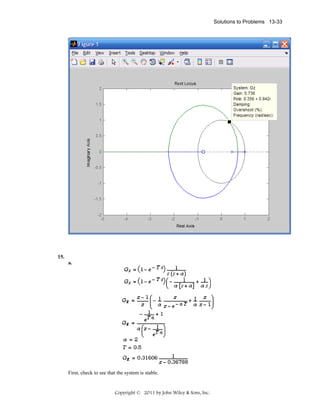
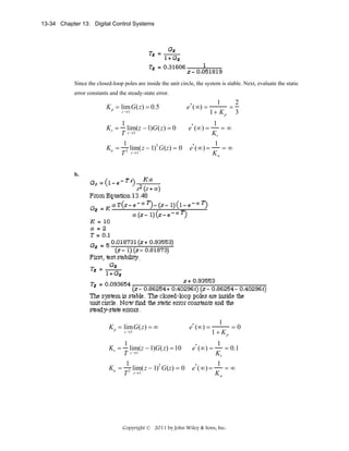
![13-36 Chapter 13: Digital Control Systems
Program:
T=0.1;
numgz=[0.04406 -0.03624 -0.03284 0.02857];
dengz=[1 -3.394 +4.29 -2.393 +0.4966];
'G(z)'
Gz=tf(numgz,dengz,0.1)
'Zeros of G(z)'
zeros=roots(numgz)
'Poles of G(z)'
poles=roots(dengz)
%Check stability
Tz=feedback(Gz,1);
'Closed-Loop Poles'
r=pole(Tz)
M=abs(r)
pause
'Find Kp'
Gz=minreal(Gz,.00001);
Kp=dcgain(Gz)
'Find Kv'
factorkv=tf([1 -1],[1 0],0.1);
%Makes transfer function
%proper and yields same Kv
Gzkv=factorkv*Gz;
Gzkv=minreal(Gzkv,.00001);
%Cancel common poles and
%zeros
Kv=(1/T)*dcgain(Gzkv)
'Find Ka'
factorka=tf([1 -2 1],[1 0 0],0.1);%Makes transfer function
%proper and yields same Ka
Gzka=factorka*Gz;
Gzka=minreal(Gzka,.00001);
%Cancel common poles and
%zeros
Ka=(1/T)^2*dcgain(Gzka)
Computer response:
ans =
G(z)
Transfer function:
0.04406 z^3 - 0.03624 z^2 - 0.03284 z + 0.02857
----------------------------------------------z^4 - 3.394 z^3 + 4.29 z^2 - 2.393 z + 0.4966
Sampling time: 0.1
ans =
Zeros of G(z)
zeros =
-0.8753
0.8489 + 0.1419i
0.8489 - 0.1419i
ans =
Poles of G(z)
poles =
Copyright © 2011 by John Wiley & Sons, Inc.](https://image.slidesharecdn.com/solutionscontrolsystemsengineeringbynormannice6ed-130502172814-phpapp02-131105052456-phpapp01/85/Solutions-control-system-sengineering-by-normannice-6ed-130502172814-phpapp02-933-320.jpg)
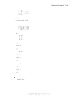
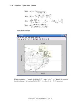
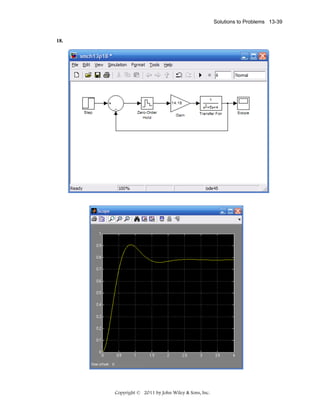
![13-40 Chapter 13: Digital Control Systems
19.
Program:
numgz=0.13*[1 1];
dengz=poly([1 0.74]);
Gz=tf(numgz,dengz,0.1)
Gzpkz=zpk(Gz)
Tz=feedback(Gz,1)
Ltiview
Computer response:
Transfer function:
0.13 z + 0.13
------------------z^2 - 1.74 z + 0.74
Sampling time: 0.1
Zero/pole/gain:
0.13 (z+1)
-------------(z-1) (z-0.74)
Sampling time: 0.1
Transfer function:
0.13 z + 0.13
------------------z^2 - 1.61 z + 0.87
Sampling time: 0.1
Copyright © 2011 by John Wiley & Sons, Inc.](https://image.slidesharecdn.com/solutionscontrolsystemsengineeringbynormannice6ed-130502172814-phpapp02-131105052456-phpapp01/85/Solutions-control-system-sengineering-by-normannice-6ed-130502172814-phpapp02-937-320.jpg)
![Solutions to Problems 13-41
20.
Program:
%Digitize G1(s) preceded by a sample and hold
numg1=1;
deng1=poly([-1 -3]);
'G1(s)'
G1s=tf(numg1,deng1)
'G(z)'
Gz=c2d(G1s,0.1,'zoh')
%Input transient response specifications
Po=input('Type %OS ');
%Determine damping ratio
z=(-log(Po/100))/(sqrt(pi^2+log(Po/100)^2));
%Plot root locus
rlocus(Gz)
zgrid(z,0)
title(['Root Locus'])
[K,p]=rlocfind(Gz) %Allows input by selecting point on graphic
pause
'T(z)'
Tz=feedback(K*Gz,1)
step(Tz)
Computer response:
ans =
G1(s)
Transfer function:
1
------------s^2 + 4 s + 3
ans =
G(z)
Transfer function:
0.004384 z + 0.003837
---------------------z^2 - 1.646 z + 0.6703
Sampling time: 0.1
Type %OS 16.3
Select a point in the graphics window
selected_point =
0.8016 + 0.2553i
K =
9.7200
p =
0.8015 + 0.2553i
0.8015 - 0.2553i
ans =
Copyright © 2011 by John Wiley & Sons, Inc.](https://image.slidesharecdn.com/solutionscontrolsystemsengineeringbynormannice6ed-130502172814-phpapp02-131105052456-phpapp01/85/Solutions-control-system-sengineering-by-normannice-6ed-130502172814-phpapp02-938-320.jpg)
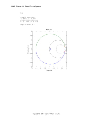
![13-46 Chapter 13: Digital Control Systems
Gc (z) =
1180z 2 − 1839z + 661.1
(z − 0.9959)(z − 0.5625)
= 1180
2
z −1
(z + 1)(z − 1)
25.
Since %OS = 10%, ζ =
%OS
- ln ( 100 )
4
= 0.591. Since Ts =
= 2 seconds,
ζωn
2 + ln2 (%OS)
π
100
ωn = 3.383 rad/s. Hence, the location of the closed-loop poles must be –2 ± j2.729. The summation of
angles from open-loop poles to –2 ± j2.729 is –192.99o. Therefore, the design point is not on the root
locus. A compensator whose angular contribution is 192.99o - 180o = 12.99o is required. Assume a
compensator zero at -5 canceling the pole at -5. Adding the compensator zero at –5 to the plant’s
poles yields –150.690 at to –2 ± j2.729. Thus, the compensator’s pole must contribute 1800 – 150.69
= 29.310. The following geometry results.
j2.729
29.31
-2
Thus,
2.729
= tan(29.310 )
pc − 2
Hence, pc = 6.86.Adding the compensator pole and zero to the system poles, the gain at the design
point is found to be 124.3. Summarizing the results:
Gc (s) =
124.3(s + 5)
. Substituting
(s + 6.86)
Eq. (13.88) into Gc(s) and letting T = 0.01 yields
Gc (z) =
123.2z − 117.2 123.2(z − 0.9512)
=
z − 0.9337
(z − 0.9337)
26.
Program:
'Design of digital lead compensation'
clf
%Clear graph on screen.
'Uncompensated System'
%Display label.
numg=1;
%Generate numerator of G(s).
deng=poly([0 -5 -8]);
%Generate denominator of G(s).
'G(s)'
%Display label.
G=tf(numg,deng)
%Create and display G(s).
pos=input('Type desired percent overshoot ');
%Input desired percent overshoot.
z=-log(pos/100)/sqrt(pi^2+[log(pos/100)]^2);
%Calculate damping ratio.
rlocus(G)
%Plot uncompensated root locus.
sgrid(z,0)
%Overlay desired percent overshoot
%line.
title(['Uncompensated Root Locus with ' , num2str(pos),...
Copyright © 2011 by John Wiley & Sons, Inc.](https://image.slidesharecdn.com/solutionscontrolsystemsengineeringbynormannice6ed-130502172814-phpapp02-131105052456-phpapp01/85/Solutions-control-system-sengineering-by-normannice-6ed-130502172814-phpapp02-943-320.jpg)
![Solutions to Problems 13-47
'% Overshoot Line'])
[K,p]=rlocfind(G);
%Title uncompensated root locus.
%Generate gain, K, and closed-loop
%poles, p, for point selected
%interactively on the root locus.
'Closed-loop poles = '
%Display label.
p
%Display closed-loop poles.
f=input('Give pole number that is operating point
');
%Choose uncompensated system
%dominant pole.
'Summary of estimated specifications for selected point on'
'uncompensated root locus'
%Display label.
operatingpoint=p(f)
%Display uncompensated dominant
%pole.
gain=K
%Display uncompensated gain.
estimated_settling_time=4/abs(real(p(f)))
%Display uncompensated settling
%time.
estimated_peak_time=pi/abs(imag(p(f)))
%Display uncompensated peak time.
estimated_percent_overshoot=pos
%Display uncompensated percent
%overshoot.
estimated_damping_ratio=z
%Display uncompensated damping
%ratio.
estimated_natural_frequency=sqrt(real(p(f))^2+imag(p(f))^2)
%Display uncompensated natural
%frequency.
numkv=conv([1 0],numg);
%Set up numerator to evaluate Kv.
denkv=deng;
%Set up denominator to evaluate Kv.
sG=tf(numkv,denkv);
%Create sG(s).
sG=minreal(sG);
%Cancel common poles and zeros.
Kv=dcgain(K*sG)
%Display uncompensated Kv.
ess=1/Kv
%Display uncompensated steady-state
%error for unit ramp input.
'T(s)'
%Display label.
T=feedback(K*G,1)
%Create and display T(s).
step(T)
%Plot step response of uncompensated
%system.
title(['Uncompensated System with ' ,num2str(pos),'% Overshoot'])
%Add title to uncompensated step
%response.
‘Press any key to go to lead compensation'
%Display label.
pause
Ts=input('Type Desired Settling Time ');
%Input desired settling time.
b=input('Type Lead Compensator Zero, (s+b). b= ');
%Input lead compensator zero.
done=1;
%Set loop flag.
while done==1
%Start loop for trying lead
%compensator pole.
a=input('Enter a Test Lead Compensator Pole, (s+a). a =
');
%Enter test lead compensator pole.
numge=conv(numg,[1 b]);
%Generate numerator of Gc(s)G(s).
denge=conv([1 a],deng);
%Generate denominator of Gc(s)G(s).
Ge=tf(numge,denge);
%Create Ge(s)=Gc(s)G(s).
wn=4/(Ts*z);
%Evaluate desired natural frequency.
clf
%Clear graph on screen.
rlocus(Ge)
%Plot compensated root locus with
%test lead compensator pole.
axis([-10,10,-10,10])
%Change lead-compensated root locus
%axes.
sgrid(z,wn)
%Overlay grid on lead-compensated
%root locus.
title(['Lead-Compensated Root Locus with ' , num2str(pos),...
'% Overshoot Line, Lead Pole at ', num2str(-a),...
' and Required Wn'])
%Add title to lead-compensated root
%locus.
Copyright © 2011 by John Wiley & Sons, Inc.](https://image.slidesharecdn.com/solutionscontrolsystemsengineeringbynormannice6ed-130502172814-phpapp02-131105052456-phpapp01/85/Solutions-control-system-sengineering-by-normannice-6ed-130502172814-phpapp02-944-320.jpg)
![13-48 Chapter 13: Digital Control Systems
done=input('Are you done? (y=0,n=1)
');
%Set loop flag.
end
%End loop for trying compensator
%pole.
[K,p]=rlocfind(Ge);
%Generate gain, K, and closed-loop
%poles, p, for point selected
%interactively on the root locus.
'Gc(s)'
%Display label.
Gc=tf([1 b],[1 a])
%Display lead compensator.
'Gc(s)G(s)'
%Display label.
Ge
%Display Gc(s)G(s).
'Closed-loop poles = '
%Display label.
p
%Display lead-compensated system's
%closed-loop poles.
f=input('Give pole number that is operating point
');
%Choose lead-compensated system
%dominant pole.
'Summary of estimated specifications for selected point on lead'
'compensated root locus'
%Display label.
operatingpoint=p(f)
%Display lead-compensated dominant
%pole.
gain=K
%Display lead-compensated gain.
estimated_settling_time=4/abs(real(p(f)))
%Display lead-compensated settling
%time.
estimated_peak_time=pi/abs(imag(p(f)))
%Display lead-compensated peak time.
estimated_percent_overshoot=pos
%Display lead-compensated percent
%overshoot.
estimated_damping_ratio=z
%Display lead-compensated damping
%ratio.
estimated_natural_frequency=sqrt(real(p(f))^2+imag(p(f))^2)
%Display lead-compensated natural
%frequency.
s=tf([1 0],1);
%Create transfer function, "s".
sGe=s*Ge;
%Create sGe(s) to evaluate Kv.
sGe=minreal(sGe);
%Cancel common poles and zeros.
Kv=dcgain(K*sGe)
%Display lead-compensated Kv.
ess=1/Kv
%Display lead-compensated steady%state error for unit ramp input.
'T(s)'
%Display label.
T=feedback(K*Ge,1)
%Create and display lead-compensated
%T(s).
'Press any key to continue and obtain the lead-compensated step'
'response'
%Display label
pause
step(T)
%Plot step response for lead
%compensated system.
title(['Lead-Compensated System with ' ,num2str(pos),'% Overshoot'])
%Add title to step response of PD
%compensated system.
pause
'Digital design'
%Print label.
T=0.01
%Define sampling interval.
clf
%Clear graph.
'Gc(s) in polynomial form'
%Print label.
Gcs=K*Gc
%Create Gc(s) in polynomial form.
'Gc(s) in polynomial form'
%Print label.
Gcszpk=zpk(Gcs)
%Create Gc(s) in factored form.
'Gc(z) in polynomial form via Tustin Transformation'
%Print label.
Gcz=c2d(Gcs,T,'tustin')
%Form Gc(z) via Tustin transformation.
'Gc(z) in factored form via Tustin Transformation'
%Print label.
Gczzpk=zpk(Gcz)
%Show Gc(z) in factored form.
'Gp(s) in polynomial form'
%Print label.
Gps=G
%Create Gp(s) in polynomial form.
Copyright © 2011 by John Wiley & Sons, Inc.](https://image.slidesharecdn.com/solutionscontrolsystemsengineeringbynormannice6ed-130502172814-phpapp02-131105052456-phpapp01/85/Solutions-control-system-sengineering-by-normannice-6ed-130502172814-phpapp02-945-320.jpg)
![Solutions to Problems 13-49
'Gp(s) in factored form'
%Print label.
Gpszpk=zpk(Gps)
%Create Gp(s) in factored form.
'Gp(z) in polynomial form'
%Print label.
Gpz=c2d(Gps,T,'zoh')
%Form Gp(z) via zoh transformation.
'Gp(z) in factored form'
%Print label.
Gpzzpk=zpk(Gpz)
%Form Gp(z) in faactored form.
pole(Gpz)
%Find poles of Gp(z).
Gez=Gcz*Gpz;
%Form Ge(z) = Gc(z)Gp(z).
'Ge(z) = Gc(z)Gp(z) in factored form'
%Print label.
Gezzpk=zpk(Gez)
%Form Ge(z) in factored form.
'z-1'
%Print label.
zm1=tf([1 -1],1,T)
%Form z-1.
zm1Gez=minreal(zm1*Gez,.00001);
%Cancel common factors.
'(z-1)Ge(z)'
%Print label.
zm1Gezzpk=zpk(zm1Gez)
%Form & display (z-1)Ge(z) in
%factored form.
pole(zm1Gez)
%Find poles of (z-1)Ge(z).
Kv=10*dcgain(zm1Gez)
%Find Kv.
Tz=feedback(Gez,1)
%Find closed-loop
%transfer function, T(z)
step(Tz)
%Find step reponse.
title('Closed-Loop Digital Step Response')
%Add title to step response.
Computer response:
ans =
Design of digital lead compensation
ans =
Uncompensated System
ans =
G(s)
Transfer function:
1
------------------s^3 + 13 s^2 + 40 s
Type desired percent overshoot 10
Select a point in the graphics window
selected_point =
-1.6435 + 2.2437i
ans =
Closed-loop poles =
p =
-9.6740
-1.6630 + 2.2492i
-1.6630 - 2.2492i
Give pole number that is operating point
2
ans =
Copyright © 2011 by John Wiley & Sons, Inc.](https://image.slidesharecdn.com/solutionscontrolsystemsengineeringbynormannice6ed-130502172814-phpapp02-131105052456-phpapp01/85/Solutions-control-system-sengineering-by-normannice-6ed-130502172814-phpapp02-946-320.jpg)
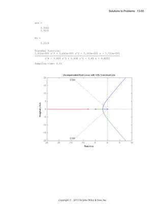
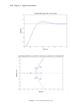
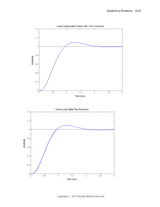
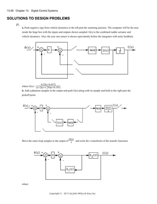
![Solutions to Problems 13-61
b.
c. The root locus intersects the unit circle at -1 with a gain, 7.9405x10⁻⁵K = 10866, or
0 < K < 136.84x10⁶.
d.
Program:
%Digitize G1(s) preceded by a sample and hold
numg1=1;
deng1=[1 7 1220 0];
'G1(s)'
G1s=tf(numg1,deng1)
'G(z)'
Gz=c2d(G1s,0.1,'zoh')
[numgz,dengz]=tfdata(Gz,'v');
'Zeros of G(z)'
roots(numgz)
'Poles of G(z)'
roots(dengz)
%Plot root locus
rlocus(Gz)
title(['Root Locus'])
[K,p]=rlocfind(Gz)
Computer response:
ans =
G1(s)
Transfer function:
1
-------------------s^3 + 7 s^2 + 1220 s
Copyright © 2011 by John Wiley & Sons, Inc.](https://image.slidesharecdn.com/solutionscontrolsystemsengineeringbynormannice6ed-130502172814-phpapp02-131105052456-phpapp01/85/Solutions-control-system-sengineering-by-normannice-6ed-130502172814-phpapp02-958-320.jpg)
![Solutions to Problems 13-63
b. Plotting the root locus. Finding the intersection with the unit circle yields 0.73576K = 1.178. Thus, 0 < K <
1.601 for stability.
c. Using the root locus, we find the intersection with the 15% overshoot curve (ζ = 0.517) at
0.5955 + j0.3747 with 0.73576K = 0.24. Thus K = 0.326.
d.
Program:
%Digitize G1(s) preceded by a sample and hold
numg1=20000;
deng1=[1 100 0];
'G1(s)'
G1s=tf(numg1,deng1)
'G(z)'
Gz=c2d(G1s,0.01,'zoh')
[numgz,dengz]=tfdata(Gz,'v');
'Zeros of G(z)'
roots(numgz)
'Poles of G(z)'
roots(dengz)
%Input transient response specifications
Po=input('Type %OS ');
%Determine damping ratio
z=(-log(Po/100))/(sqrt(pi^2+log(Po/100)^2))
%Plot root locus
rlocus(Gz)
zgrid(z,0)
title(['Root Locus'])
[K,p]=rlocfind(Gz) %Allows input by selecting point on graphic.
Computer response:
ans =
G1(s)
Transfer function:
20000
----------s^2 + 100 s
Copyright © 2011 by John Wiley & Sons, Inc.](https://image.slidesharecdn.com/solutionscontrolsystemsengineeringbynormannice6ed-130502172814-phpapp02-131105052456-phpapp01/85/Solutions-control-system-sengineering-by-normannice-6ed-130502172814-phpapp02-960-320.jpg)
![13-66 Chapter 13: Digital Control Systems
The characteristic equation for this system is:
1 + G( z) = 1 +
(0.0031z 2 + 0.0031z + 0.0104) K
= 0 or
( z − 0.953)( z − 0.8279)
(1 + 0.0031K ) z 2 + (0.0031K − 1.7809) z + (0.789 + 0.0104 K ) = 0
s '+1
We use now the bilinear transformation by substituting z =
s '−1
2
( s '+1)
s '+1
(1 + 0.0031K )
+ (0.0031K − 1.7809)
+ (0.789 + 0.0104 K ) = 0
2
s '−1
( s '−1)
giving
(0.0081 + 0.0166 K ) s ' 2 +(0.422 − 0.0146 K ) s '+(3.5699 + 0.0104 K ) = 0
The Routh array is
s'2
0.0081 + 0.0166 K
s'
0.422 − 0.0146 K
1
3.5699 + 0.0104 K
3.5699 + 0.0104 K
The first column of the array will be >0 when K>0 and from the second row
K<
0.422
= 28.9041
0.0146
So the system is closed loop stable when 0 < K < 28.9041 .
32.
a. In Problem 31 we found that for this system with T=1sec, G ( z ) =
K (0.0031z 2 + 0.0031z + 0.0104)
( z − 0.953)( z − 0.8279)
In MATLAB this system is defined as G=tf(0.0031*[1 1 3.3548],conv([1 -0.953],[1 -0.8279]),1). Invoking
SISOTOOL one gets
Copyright © 2011 by John Wiley & Sons, Inc.](https://image.slidesharecdn.com/solutionscontrolsystemsengineeringbynormannice6ed-130502172814-phpapp02-131105052456-phpapp01/85/Solutions-control-system-sengineering-by-normannice-6ed-130502172814-phpapp02-963-320.jpg)
![Solutions to Problems 13-67
Root Locus Editor for Open Loop 1 (OL1)
2
1.5
1
1.88
1.57
1.26
0.1
2.2
2.51
0.5
2.83
Imag Axis
0.942
0.2
0.3
0.4
0.5
0.6
0.7
0.8
0.9
0.628
0.314
3.14
3.14
0
2.83
-0.5
0.314
2.51
0.628
2.2
0.942
1.88
-1
1.57
1.26
-1.5
-2
-2
b.
-1.5
ζ = 0.7
-1
-0.5
0
Real Axis
0.5
1
1.5
2
is achieved when K=0.928
c. The closed loop poles are located at 0.866±j0.103. The radial distance from the origin is
− 4T
= 29.2 sec . The radial angle from the origin is
ln(r )
Tp π
π
0.103
θ1 = tan −1
= 6.8 o = 0.12rad , so
=
=
= 26.54 or T p = 26.54 sec
0.866
T θ1 0.12
r = 0.866 2 + 0.103 2 = 0.872 , so Ts =
d. We have that K p = Lim G ( z ) = Lim
z →1
error is e ss =
z →1
(0.928)(0.0031)(z 2 + z + 3.3548) = 1.905 . The steady state
( z − 0.953)( z − 0.8279)
1
= 0.344 . Then c(∞) = 1 − 0.344 = 0.655
1+ K p
e.
1
0.928
0.0031*[1 1 3.3548]
conv([1 -0.953],[1 -0.8279])(z)
Constant
Gain
Discrete
Transfer Fcn
Zero-Order
Hold
Copyright © 2011 by John Wiley & Sons, Inc.
Scope](https://image.slidesharecdn.com/solutionscontrolsystemsengineeringbynormannice6ed-130502172814-phpapp02-131105052456-phpapp01/85/Solutions-control-system-sengineering-by-normannice-6ed-130502172814-phpapp02-964-320.jpg)
![Solutions to Problems 13-69
c.
0.5*[1 1.63]
conv([1/305.4^2 0.36/305.4 1],[1/248.2^2 0.04/248.2 1])(s)
M(s)
1
0.63
s2 +0.27s
P(s)2
Constant
Scope
0.07278*[1 0.3386 -0.6614]
0.63
z2 -1.935z+0.9347
conv([1/305.4^2 0.36/305.4 1],[1/248.2^2 0.04/248.2 1])(s)
M(z)
Zero-Order
Hold
P(s)1
Copyright © 2011 by John Wiley & Sons, Inc.](https://image.slidesharecdn.com/solutionscontrolsystemsengineeringbynormannice6ed-130502172814-phpapp02-131105052456-phpapp01/85/Solutions-control-system-sengineering-by-normannice-6ed-130502172814-phpapp02-966-320.jpg)
![Solutions to Problems 13-71
35.
a. With the zero order hold the open loop transfer function is
G1 ( s ) =
(1 − e −0.5 s ) K
s ( s + 0.08)( s + 2)( s + 5)
⎡1.25 1.3233 0.0868 0.0136 ⎤
= (1 − e −0.5 s ) K ⎢
−
+
−
s + 0.08
s+2
s+5 ⎥
⎣ s
⎦
z − 1 ⎡1.25 z 1.3233 z
0.0868 z
0.0136 z ⎤
G( z) = K
⎢ z − 1 − z − 0.961 + z − 0.368 − z − 0.0821⎥
z ⎣
⎦
=
− 1 × 10 − 4 K ( z 3 − 94 z 2 − 174 z − 16)
− 1 × 10 − 4 K ( z 3 − 94 z 2 − 174 z − 16)
== 3
( z − 0.0821)( z − 0.368)( z − 0.961)
z − 1.411z 2 + 0.4628 z − 0.02903
In MATLAB this system is defined as G=tf(-1e-4*[1 -94 -174 -16],[1 -1.411 0.4628 -0.02903]),0.5). Invoking
SISOTOOL one gets
Copyright © 2011 by John Wiley & Sons, Inc.](https://image.slidesharecdn.com/solutionscontrolsystemsengineeringbynormannice6ed-130502172814-phpapp02-131105052456-phpapp01/85/Solutions-control-system-sengineering-by-normannice-6ed-130502172814-phpapp02-968-320.jpg)
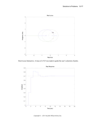
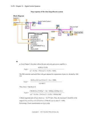
![Solutions to Problems 13-79
5.166e04 z4 - 2.041e05 z3 + 3.029e05 z2 - 2.001e05 z + 4.963e04
Gc(z) = -----------------------------------------------------------------------------------------Z4 - 1.883 z3 - 0.1131 z2 + 1.883 z - 0.8869
b. Drawing the flowchart
5.166e4
-2.041e5
-1.883
+ ++
- --
3.029e5
-0.1131
1.883
-2.001e5
-0.8869
4.963e4
T = 0.001
c.
Program:
syms s
'Compensator from Chapter 9'
T=.001
Gc=26.82*(s^2+16*s+9200)*(s+24.09)*(s+.1)/(s*((s+60)^2));
Gc=vpa(Gc,4);
[numgc,dengc]=numden(Gc);
numgc=sym2poly(numgc);
dengc=sym2poly(dengc);
Copyright © 2011 by John Wiley & Sons, Inc.](https://image.slidesharecdn.com/solutionscontrolsystemsengineeringbynormannice6ed-130502172814-phpapp02-131105052456-phpapp01/85/Solutions-control-system-sengineering-by-normannice-6ed-130502172814-phpapp02-976-320.jpg)
![13-80 Chapter 13: Digital Control Systems
Gc=tf(numgc,dengc);
'Gc(s)'
Gczpk=zpk(Gc)
'Gc(z)'
Gcz=c2d(Gc,T,'tustin')
'Gc(z)'
Gczzpk=zpk(Gcz)
'Plant from Chapter 9'
Gp=64.88*(s+53.85)/[(s^2+15.47*s+9283)*(s^2+8.119*s+376.3)];
Gp=vpa(Gp,4);
[numgp,dengp]=numden(Gp);
numgp=sym2poly(numgp);
dengp=sym2poly(dengp);
'Gp(s)'
Gp=tf(numgp,dengp)
'Gp(s)'
Gpzpk=zpk(Gp)
'Gp(z)'
Gpz=c2d(Gp,T,'zoh')
'Gez=Gcz*Gpz'
Gez=Gcz*Gpz
Tz=feedback(Gez,1);
t=0:T:1;
step(Tz,t)
pause
t=0:T:50;
step(Tz,t)
Computer response:
ans =
Compensator from Chapter 9
T =
0.0010
ans =
Gc(s)
Zero/pole/gain:
26.82 (s+24.09) (s+0.1) (s^2 + 16s + 9198)
------------------------------------------s (s+60)^2
ans =
Gc(z)
Transfer function:
5.17e004 z^4 - 2.043e005 z^3 + 3.031e005 z^2 - 2.002e005 z + 4.966e004
---------------------------------------------------------------------z^4 - 1.883 z^3 - 0.1131 z^2 + 1.883 z - 0.8869
Sampling time: 0.001
ans =
Gc(z)
Copyright © 2011 by John Wiley & Sons, Inc.](https://image.slidesharecdn.com/solutionscontrolsystemsengineeringbynormannice6ed-130502172814-phpapp02-131105052456-phpapp01/85/Solutions-control-system-sengineering-by-normannice-6ed-130502172814-phpapp02-977-320.jpg)
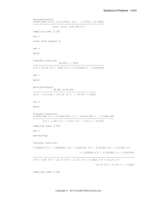
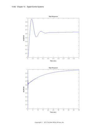
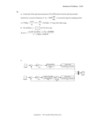
![13-84 Chapter 13: Digital Control Systems
42.
a. The following MATLAB M-file was developed
%Digitize G1(s) preceded by a sample and hold
%Input transient response specifications
Po=input('Type %OS ');
K = input('Type Proportional Gain of PI controller
numg1 = K*poly([-0.01304 -0.6]);
deng1 = poly([0 -0.01631 -0.5858]);
G1 = tf(numg1,deng1);
for T=5:-.01:0;
Gz=c2d(G1,T,'zoh');
Copyright © 2011 by John Wiley & Sons, Inc.
');](https://image.slidesharecdn.com/solutionscontrolsystemsengineeringbynormannice6ed-130502172814-phpapp02-131105052456-phpapp01/85/Solutions-control-system-sengineering-by-normannice-6ed-130502172814-phpapp02-981-320.jpg)
![Solutions to Problems 13-85
Tz=feedback(Gz,1);
r=pole(Tz);
rm=max(abs(r));
if rm<=1;
break;
end;
end;
'G1(s)';
G1s=tf(numg1,deng1);
'G(z)';
Gz=c2d(G1s,0.75*T,'zoh');
%Determine damping ratio
z=(-log(Po/100))/(sqrt(pi^2+log(Po/100)^2));
%Plot root locus
rlocus(Gz)
zgrid(z,0)
title('Root Locus')
[K,p]=rlocfind(Gz); %Allows input by selecting point on graphic
pause
'T(z)';
Tz=feedback(K*Gz,1);
step(Tz)
b. As the M-file developed in (a) was run and the values of the desired percent overshoot, %O.S. = 0, and PI
speed controller’s proportional gain, K = 61 were entered, the root locus, shown below, was obtained.
c. A point was selected on the root locus such that is inside the unit circle. That point is: 0.9837 + 0.0000i
d. The sampled data transfer functions, Gz and Tz, obtained at a Sampling time, T = 0.0225 = 0.75*0.03 are:
Copyright © 2011 by John Wiley & Sons, Inc.](https://image.slidesharecdn.com/solutionscontrolsystemsengineeringbynormannice6ed-130502172814-phpapp02-131105052456-phpapp01/85/Solutions-control-system-sengineering-by-normannice-6ed-130502172814-phpapp02-982-320.jpg)
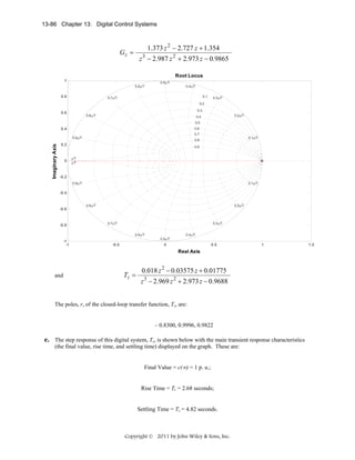
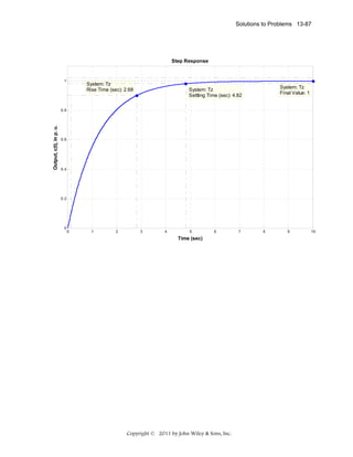

This document is a solutions manual for an unknown textbook. It contains 20 solved problems related to control systems and feedback loops. The problems cover various concepts like modeling systems using differential equations, determining transfer functions and state-space representations, analyzing stability, and designing feedback loops. John Wiley & Sons is identified as the publisher.


![Reduction of multiple subsystem [compatibility mode]](https://cdn.slidesharecdn.com/ss_thumbnails/reductionofmultiplesubsystemcompatibilitymode-110418075355-phpapp01-thumbnail.jpg?width=640&height=640&fit=bounds)