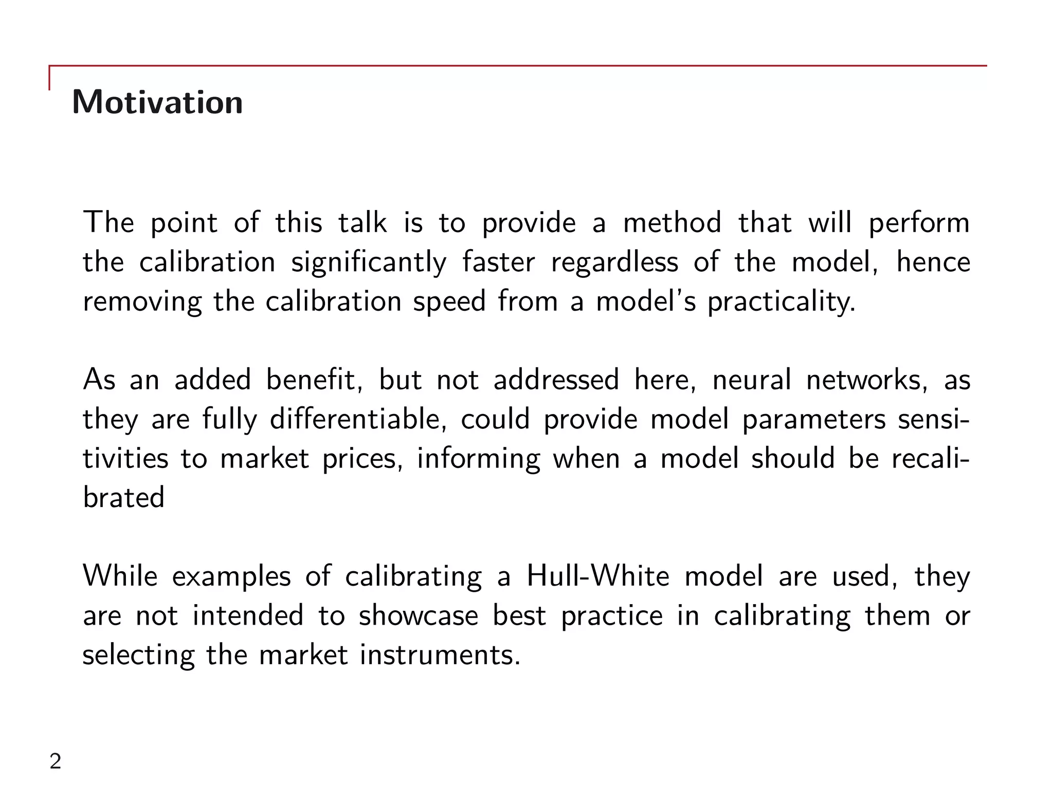
The document outlines a method for model calibration using neural networks, aimed at improving the speed and efficiency of the calibration process across various models. It discusses the calibration problem, supervised and unsupervised training approaches, and provides examples related to the Hull-White model while noting potential benefits such as sensitivity analysis to market prices. Future work includes refining bespoke optimizers and exploring applications in local stochastic volatility models.

1. Model Calibration with
Neural Networks
Andres Hernandez

2. Motivation
The point of this talk is to provide a method that will perform
the calibration significantly faster regardless of the model, hence
removing the calibration speed from a model’s practicality.
As an added benefit, but not addressed here, neural networks, as
they are fully differentiable, could provide model parameters sensi-
tivities to market prices, informing when a model should be recali-
brated
While examples of calibrating a Hull-White model are used, they
are not intended to showcase best practice in calibrating them or
selecting the market instruments.
2

3. Table of contents
1 Background
Calibration Problem
Example: Hull-White
Neural Networks
2 Supervised Training
Approach
Training
Neural Network Topology
Results
Generating Training Set
3 Unsupervised Training
Approach
Reinforcement Learning
Neural networks training
other neural networks
3

4. Background

5. Definition
Model calibration is the process by which model parameters are ad-
justed to ’best’ describe/fit known observations. For a given model
M, an instrument’s theoretical quote is obtained
Q(τ) = M(θ; τ, ϕ),
where θ represents the model parameters, τ represents the identify-
ing properties of the particular instrument, e.g. maturity, day-count
convention, etc., and ϕ represents other exogenous factors used for
pricing, e.g. interest rate curve.
5

6. Definition
The calibration problem consists then in finding the parameters θ,
which best match a set of quotes
θ = arg min
θ∗∈S⊆Rn
Cost
(
θ∗
, {ˆQ}; {τ}, ϕ
)
= Θ
(
{ˆQ}; {τ}, ϕ
)
,
where {τ} is the set of instrument properties and {ˆQ} is the set of
relevant market quotes
{ˆQ} = {ˆQi|i = 1 . . . N}, {τ} = {τi|i = 1 . . . N}
The cost can vary, but is usually some sort of weighted average of
all the errors
Cost
(
θ∗
, {ˆQ}; {τ}, ϕ
)
=
N∑
i=1
wi(Q(τi) − ˆQ(τi))2
6

7. Definition
The calibration problem can be seen as a function with N inputs and
n outputs
Θ : RN
→ Rn
It need not be everywhere smooth, and may in fact contain a few
discontinuities, either in the function itself, or on its derivatives,
but in general it is expected to be continuous and smooth almost
everywhere. As N can often be quite large, this presents a good use
case for a neural network.
7

8. Hull-White Model
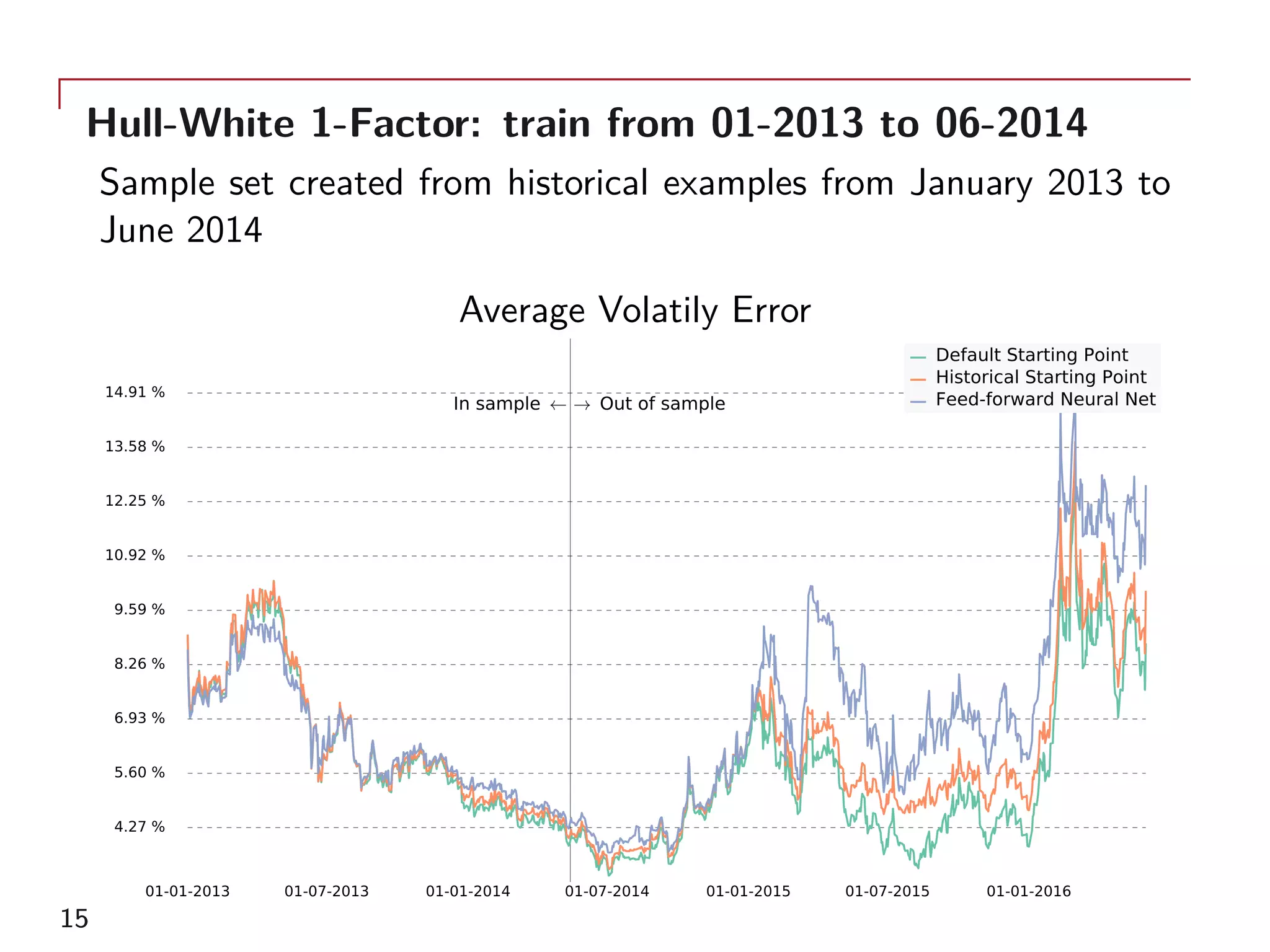
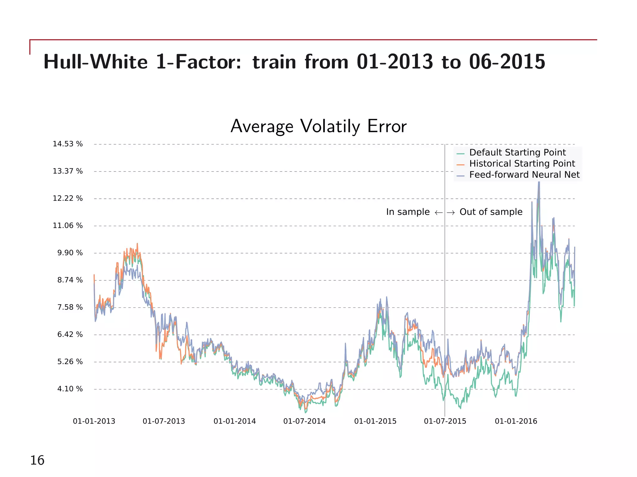
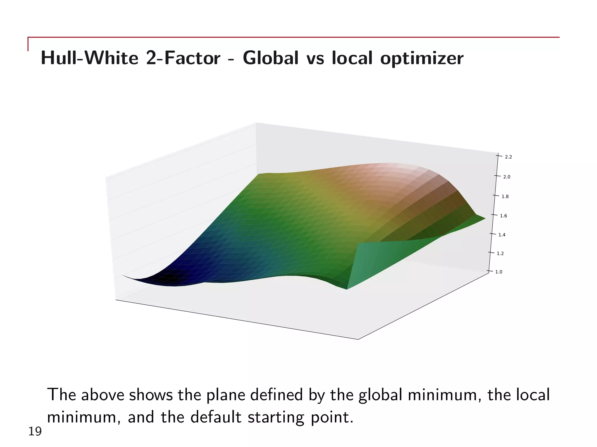
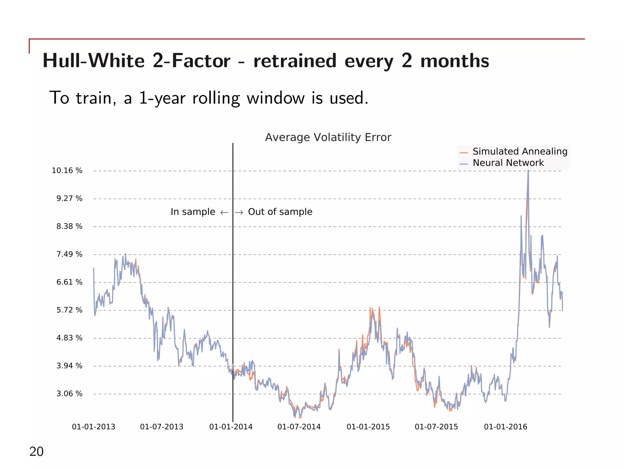
As examples, the single-factor Hull-White model and two-factor
model calibrated to 156 GBP ATM swaptions will be used
drt = (θ(t) − αrt)dt + σdWt drt = (θ(t) + ut − αrt) dt + σ1dW1
t
dut = −butdt + σ2dW2
t
with dW1
t dW2
t = ρdt. All parameters, α, σ, σ1, σ2, and b are
positive, and shared across all option maturities. ρ ∈ [−1, 1]. θ(t)
is picked to replicate the current yield curve y(t).
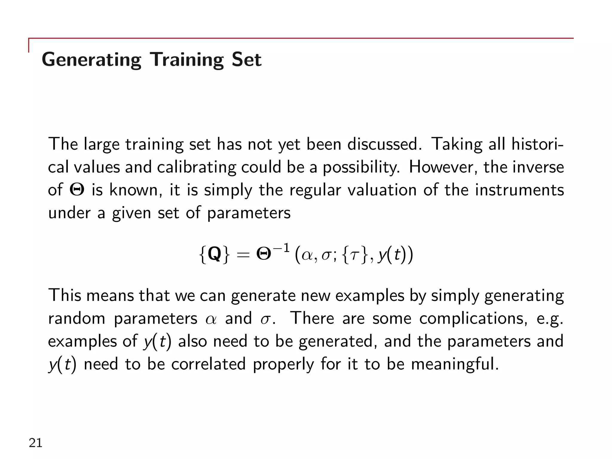
The related calibration problems are then
(α, σ) = Θ1F
(
{ˆQ}; {τ}, y(t)
)
(α, σ1, σ2, b, ρ) = Θ2F
(
{ˆQ}; {τ}, y(t)
)
8

9. Artificial neural networks
Artificial neural networks are a family of machine learning tech-
niques, which are currently used in state-of-the-art solutions for im-
age and speech recognition, and natural language processing.
In general, artificial neural networks are an extension of regression
aX + b aX2 + bX + c
1
1+exp(−a(X−b))
9

10. Neural Networks
In neural networks, independent regression units are stacked together
in layers, with layers stacked on top of each other
10

11. Supervised Training Approach

12. Calibration through neural networks
The calibration problem can been reduced to finding a neural net-
work to approximate Θ. The problem is split into two: a training
phase, which would normally be done offline, and the evaluation,
which gives the model parameters for a given input
Training phase:
1 Collect large training set of calibrated examples
2 Propose neural network
3 Train, validate, and test it
Calibration of a model would then proceed simply by applying the
previously trained Neural Network on the new input.
12

13. Supervised Training
If one is provided with a set of associated input and output samples,
one can ’train’ the neural network’s to best be able to reproduce the
desired output given the known inputs.
The most common training method are variations of gradient de-
scent. It consists of calculating the gradient, and moving along in
the opposite direction. At each iteration, the current position is xm
is updated so
xm+1 = xm − γ∇F(xm),
with γ called learning rate. What is used in practice is a form of
stochastic gradient descent, where the parameters are not updated
after calculating the gradient for all samples, but only for a random
small subsample.
13

14. Feed-forward neural network for 2-factor HW
Input
SWO
156×1
IR
44×1
Hidden Layer
a1 =
elu(W1 · BN(p) + b1)
p
200 × 1
BN1
64 × 200 W1
1
64 × 1
b1
+
DO1
+
Hidden Layer (x8)
ai = ai−1+
elu(Wi · BN(ai−1) + bi)
BNi
Wi
1
64 × 1
bi
+
DOi
+
Output Layer
a10 = W10 · a9 + b10
DO10
5 × 64
W10
1
5 × 1
b1
+
14

15. Hull-White 1-Factor: train from 01-2013 to 06-2014
Sample set created from historical examples from January 2013 to
June 2014
Average Volatily Error
01-01-2013 01-07-2013 01-01-2014 01-07-2014 01-01-2015 01-07-2015 01-01-2016
4.27 %
5.60 %
6.93 %
8.26 %
9.59 %
10.92 %
12.25 %
13.58 %
14.91 %
→ Out of sampleIn sample ←
Default Starting Point
Historical Starting Point
Feed-forward Neural Net
15

16. Hull-White 1-Factor: train from 01-2013 to 06-2015
Average Volatily Error
01-01-2013 01-07-2013 01-01-2014 01-07-2014 01-01-2015 01-07-2015 01-01-2016
4.10 %
5.26 %
6.42 %
7.58 %
8.74 %
9.90 %
11.06 %
12.22 %
13.37 %
14.53 %
→ Out of sampleIn sample ←
Default Starting Point
Historical Starting Point
Feed-forward Neural Net
16

17. Cost Function on 01-07-2015
The historical point, lies on the trough. The default starting point
(α = 0.1, σ = 0.01) starts up on the side.
17

18. Hull-White 2-Factor
Comparison of local optimizer against global optimizer
01-01-2013 01-07-2013 01-01-2014 01-07-2014 01-01-2015 01-07-2015 01-01-2016
3 %
4 %
5 %
6 %
7 %
8 %
9 %
10 %
11 %
12 %
Average Volatility Error
Local optimizer
Global optimizer
18

19. Hull-White 2-Factor - Global vs local optimizer
1.0
1.2
1.4
1.6
1.8
2.0
2.2
The above shows the plane defined by the global minimum, the local
minimum, and the default starting point.
19

20. Hull-White 2-Factor - retrained every 2 months
To train, a 1-year rolling window is used.
01-01-2013 01-07-2013 01-01-2014 01-07-2014 01-01-2015 01-07-2015 01-01-2016
3.06 %
3.94 %
4.83 %
5.72 %
6.61 %
7.49 %
8.38 %
9.27 %
10.16 %
→ Out of sampleIn sample ←
Average Volatility Error
Simulated Annealing
Neural Network
20

21. Generating Training Set
The large training set has not yet been discussed. Taking all histori-
cal values and calibrating could be a possibility. However, the inverse
of Θ is known, it is simply the regular valuation of the instruments
under a given set of parameters
{Q} = Θ−1
(α, σ; {τ}, y(t))
This means that we can generate new examples by simply generating
random parameters α and σ. There are some complications, e.g.
examples of y(t) also need to be generated, and the parameters and
y(t) need to be correlated properly for it to be meaningful.
21

22. Generating Training Set
The intention is to collect historical examples, and imply some kind
of statistical model from them, and then draw from that distribution.
1 Calibrate model for training history
2 Obtain errors for each instrument for each day
3 As parameters are positive, take logarithm on the historical
values
4 Rescale yield curves, parameters, and errors to have zero
mean and variance 1
5 Apply dimensional reduction via PCA to yield curve, and keep
parameters for given explained variance (e.g. 99.5%)
22

23. Generating Training Set - From normal distribution
6 Calculate covariance of rescaled log-parameters, PCA yield
curve values, and errors
7 Generate random normally distributed vectors consistent with
given covariance
8 Apply inverse transformations: rescale to original mean,
variance, and dimensionality, and take exponential of
parameters
9 Select reference date randomly
10 Obtain implied volatility for all swaptions, and apply random
errors
23

24. Generating Training Set - Variational autoencoder
Variational autoen-
coders learn a la-
tent variable model
that parametrizes a
probability distribu-
tion of the output
contingent on the
input.
24

25. Normal distribution vs variational autoencoder (no
retraining)
01-01-2013 01-07-2013 01-01-2014 01-07-2014 01-01-2015 01-07-2015 01-01-2016
3.70 %
5.22 %
6.75 %
8.27 %
9.80 %
11.33 %
12.85 %
14.38 %
15.90 %
→ Out of sampleIn sample ←
Average Volatility Error
Global Optimizer
FNN with Normal Dist.
FNN with VAE
25

26. Unsupervised Training Approach

27. Bespoke optimizer
But what about the case where one doesn’t have a long time-series?
Reinforcement learning can be used to create better bespoke opti-
mizers than the traditional local or global optimization procedures.
27

28. Deep-q learning
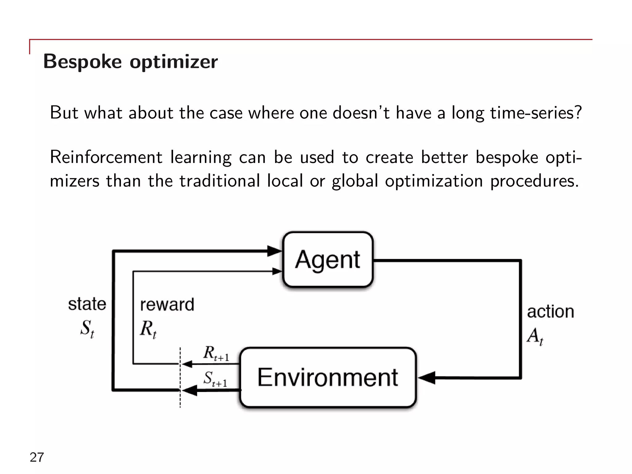
A common approach for reinforcement learning with a large possi-
bility of actions and states is called Q-Learning:
An agent’s behaviour is defined by a policy π, which maps states to
a probability distribution over the actions π : S → P(A).
The return Rt from an action is defined as the sum of discounted
future rewards Rt =
∑T
i=t γi−tr(si, ai).
The quality of an action is the expected return of an action at in
state st
Qπ
(at, st) = Eri≥t,si>t,ai>t [Rt|st, at]
28

29. Learning to learn without gradient descent with
gradient descent
A long-short-term memory (LSTM)
architecture was used to simplify
represent the whole agent. The
standard LSTM block is composed of
several gates with an internal state:
In the current case,
100 LSTM blocks were
used per layer, and 3
layers were stacked on
top of each other
t
29

30. Unrolled recurrent network
30

31. Train the optimizer
Train it with approximation of
F(x), whose gradient is available
Advantage: training proceeds fast
Disadvantage: potentially will
not reach full possibility
Train it with non-gradient based
optimizer
Local optimizer: generally
requires a number of evaluations
∼ to number of dimensions to
take next step
Global optimizer: very hard to
set hyperparameters
Train a second NN to train first NN
31

32. Bespoke optimizer
01-01-2013 01-07-2013 01-01-2014 01-07-2014 01-01-2015 01-07-2015
2.67 %
3.85 %
5.03 %
6.21 %
7.39 %
8.57 %
9.74 %
10.92 %
12.10 %
→ Out of sampleIn sample ←
Average Volatility Error
Neural Network
Global optimizer
32

33. References
https://github.com/Andres-Hernandez/CalibrationNN
A. Hernandez, Model calibration with neural networks, Risk,
June 2017
A. Hernandez, Model Calibration: Global Optimizer vs.
Neural Network, SSRN abstract id=2996930
Y. Chen, et al Learning to Learn without Gradient Descent by
Gradient Descent, arXiv:1611.03824
33

34. Future work
Calibration of local stochastic volatility model. Work is being
undertaken in collaboration with Professors J. Teichmann
from the ETH Zürich, and C. Cuchiero in University of Wien,
and W. Khosrawi-Sardroudi from the University of Freiburg.
Improvement of bespoke optimizers, in particular train with
more random environment: different currencies, constituents,
etc.
Use of bespoke optimizer as large-dimensional PDE solver
34

35. ®2017 PricewaterhouseCoopers GmbH Wirtschaftsprüfungsgesellschaft. All rights reserved. In this
document, “PwC” refers to PricewaterhouseCoopers GmbH Wirtschaftsprüfungsgesellschaft, which is a
member firm of PricewaterhouseCoopers International Limited (PwCIL). Each member firm of PwCIL is a
separate and independent legal entity.