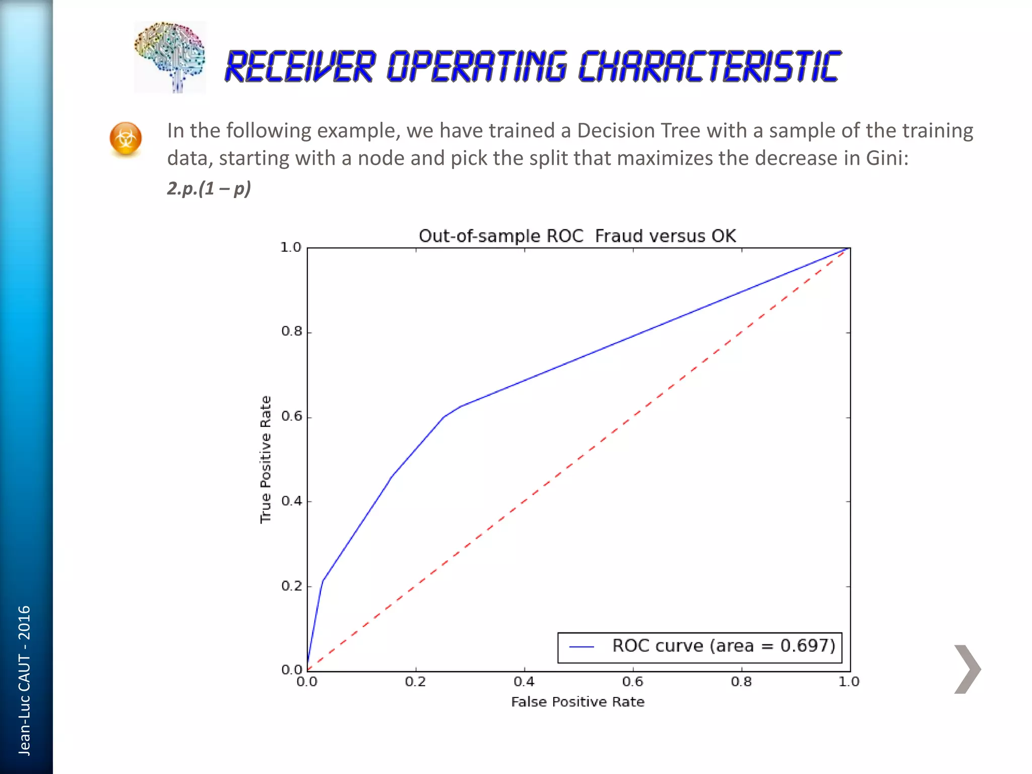
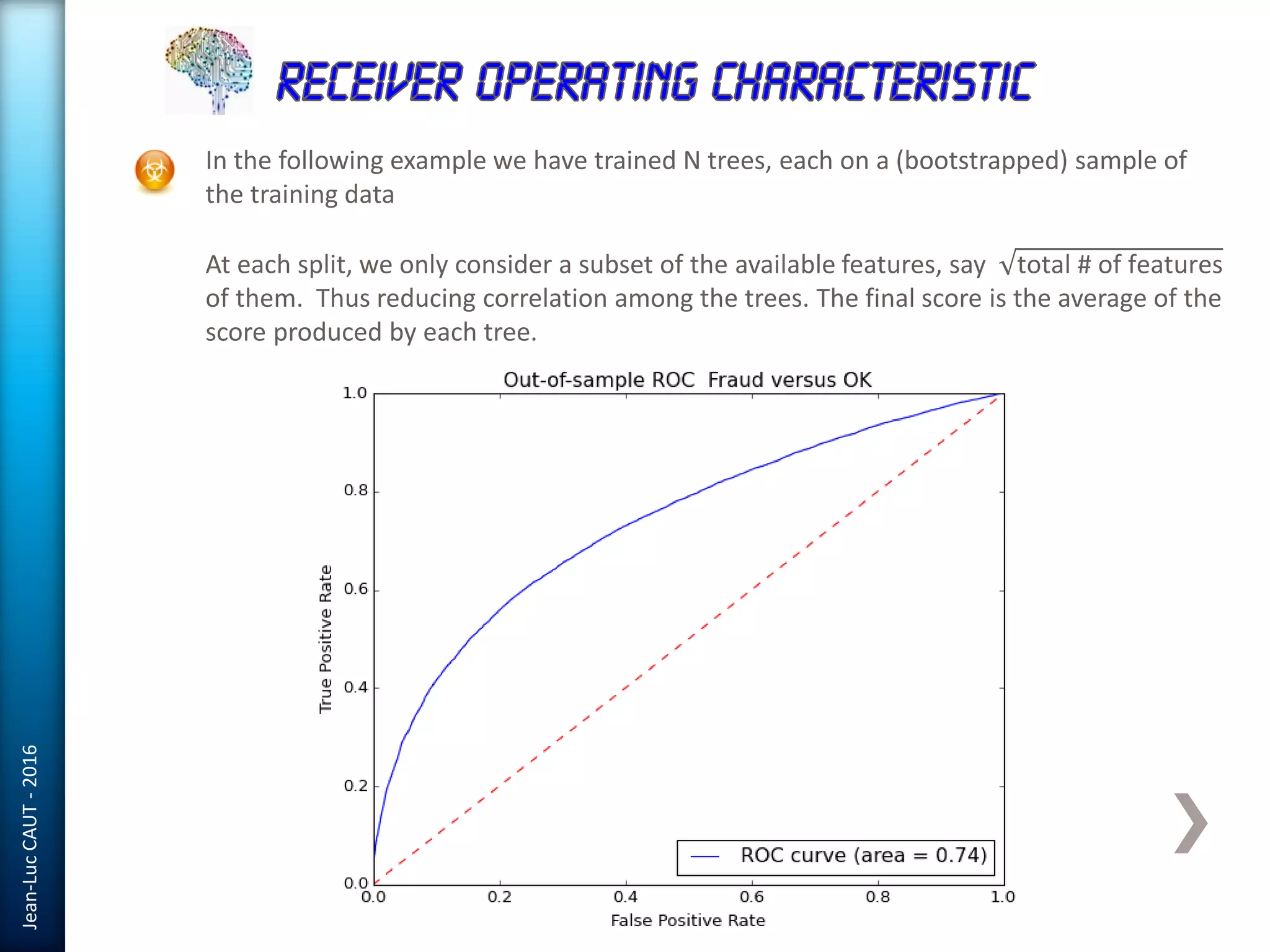
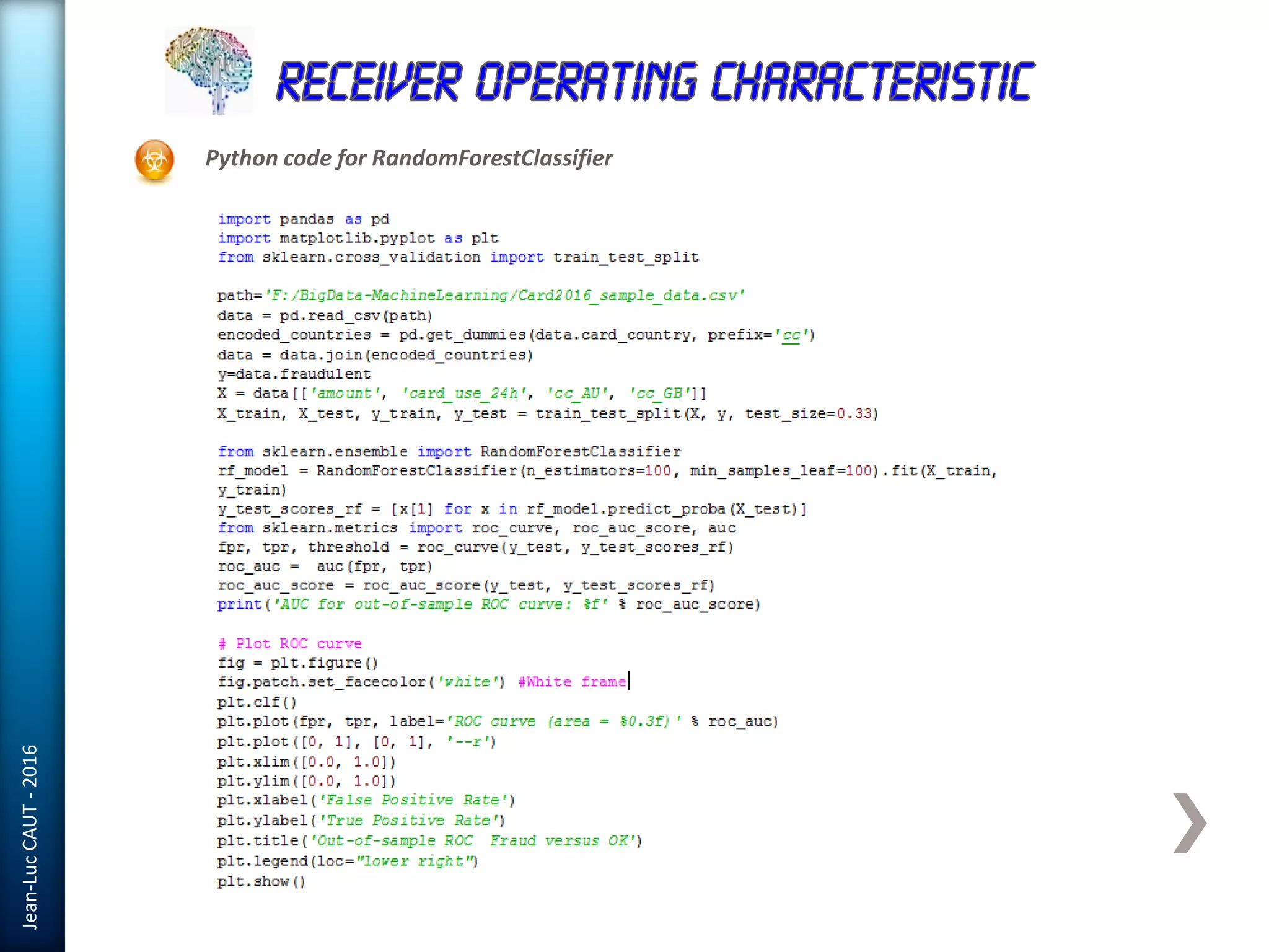
SlideShare a Scribd company logo
Jean-LucCAUT-2016
Help Banks to detect Suspicious Transaction & Fraud
Jean-LucCAUT-2016
Introduction
Supervised learning models
Confusion matrix
Unsupervised models
Jean-LucCAUT-2016
Introduction
Supervised learning models
Confusion Matrix
Unsupervised models
Jean-LucCAUT-2016
Machine Learning
is a subfield of Computer Science that evolved from the study of pattern
recognition and computational learning theory in artificial intelligence.
In 1959 Arthur Samuel, defined machine learning as a:
"Field of study that gives computers the ability to learn without being
explicitly programmed.”
Let’s go further and have look on what is hidden behind the scenes.
Jean-LucCAUT-2016
Machine Learning is often used to build predictive models by extracting patterns
from large datasets.
These models are used in predictive data analytics applications including price
prediction, risk assessment, predicting customer behavior, and document
classification.
This presentation offers a detailed and focused treatment of one the most
important machine learning approach used in predictive data analytics,
covering both theoretical concepts and practical applications.
Technical and mathematical material is augmented with explanatory worked
example developed in Python in order to illustrate the application of these
models in the financial business context.
Jean-LucCAUT-2016
Machine Learning tasks are typically classified into three broad categories,
depending on the nature of the learning "signal" or "feedback" available to a
learning system. These are:
Supervised learning: The computer is presented with example inputs and their
desired outputs, given by a "teacher", and the goal is to learn a general rule that
maps inputs to outputs.
Unsupervised learning: No labels are given to the learning algorithm, leaving it on its
own to find structure in its input. Unsupervised learning can be a goal in itself
(discovering hidden patterns in data) or a means towards an end (feature learning).
Reinforcement learning: A computer program interacts with a dynamic environment
in which it must perform a certain goal (such as driving a vehicle), without a teacher
explicitly telling it whether it has come close to its goal. Another example is learning
to play a game by playing against an opponent.
Jean-LucCAUT-2016
Visualizing the important characteristics of a dataset
Exploratory Data Analysis (EDA) is an important and recommended first step prior to the
training of a machine learning model.
First, we will create a scatterplot matrix that allows us to visualize the pair-wise
correlations between the different features in this dataset in one place.
Jean-LucCAUT-2016
Correlation Matrix
To quantify the linear relationship between the features, we will now create a correlation
matrix.
The correlation matrix is a square matrix that contains the Pearson product-
moment correlation coefficients (often abbreviated as Pearson's r), which measure
the linear dependence between pairs of features.
For example, we can see that
there is a linear relationship
between RM and the
housing prices MEDV.
Or between NOX emission
and the surface of industries
INDUS.
Jean-LucCAUT-2016
Introduction
Supervised learning models
Confusion Matrix
Unsupervised models
Jean-LucCAUT-2016
Supervised learning is the machine learning task of inferring a function from
labeled training data. The computer is presented with example inputs and their
desired outputs, given by a "teacher", and the goal is to learn a general rule
that maps inputs to outputs.
The training data consist of a set of training examples. In supervised learning, each
example is a pair consisting of an input object (typically a vector) and a desired
output value (also called the supervisory signal).
A supervised learning algorithm analyzes the training data and produces an inferred
function, which can be used for mapping new examples. An optimal scenario will
allow for the algorithm to correctly determine the class labels for unseen instances.
This requires the learning algorithm to generalize from the training data to unseen
situations in a "reasonable" way .
Jean-LucCAUT-2016
Determine the type of training
examples
Gather a training set.
Determine the input feature
representation of the learned
function.
Determine the structure of the
learned function and corresponding
learning algorithm.
Run the learning algorithm on the
gathered training set.
Evaluate the accuracy of the
learned function.
Learning Process
Jean-LucCAUT-2016
A quick look at our dataset allows us
to notice that Petal length and width
could be good candidates for our
classification.
This step called dimensionality
reduction of our feature space. The
main advantage is that the learning
algorithm will run much faster.
A potential use of supervised learning model is classification.
The Iris dataset is a classic example in the field of machine learning, it contains the
measurements of 150 iris flowers from three different species: Setosa, Versicolor, and
Viriginica.
Here, each flower Sample represents one row in our data set, and the flower
measurements in centimeters are stored as columns, which we also call the Features of the
dataset.
Data set is available at: https://archive.ics.uci.edu/ml/machine-learning-databases/iris/iris.data
Jean-LucCAUT-2016
Many different machine learning algorithms have been developed to solve different
problem tasks.
An important point that can be summarized from David Wolpert's famous No Free Lunch
Theorems is that we can't get learning "for free" (The Lack of A Priori Distinctions Between Learning
Algorithms, D.H. Wolpert 1996; No Free Lunch Theorems for Optimization, D.H. Wolpert and W.G. Macready, 1997).
For example, each classification algorithm has its inherent biases, and no single
classification model enjoys superiority if we don't make any assumptions about the task.
In practice, it is therefore essential to compare at least a handful of different algorithms in
order to train and select the best performing model.
“Would you tell me, please,
which way I ought to go from here?” Said Alice
“That depends a good deal on where you want to get to,” said the Cat.
Alice in Wonderland, Lewis Carroll
Jean-LucCAUT-2016
Linear classification model
the Logistic Regression and the conditional probabilities
Logistic regression is the most widely used algorithms for classification in industry. It is very
easy to implement but performs very well on linearly separable classes.
To explain the idea behind logistic regression as a probabilistic model, let's first introduce
the odds ratio, which is the odds in favor of a particular event.
The term positive event does refers to the event that we want to predict, e.g. the
probability that a patient has a certain disease. We can then further define he logit
function, which is simply the logarithm of the odds ratio where p stands for the probability
of the positive event.
The logit function takes input values in the range 0 to 1 and transforms them to values over
the entire real number range, which we can use to express a linear relationship between
feature values and the log-odds:
Jean-LucCAUT-2016
Then we are interested in predicting the probability that a certain sample belongs to a
particular class, which is the inverse form of the logit function. It is also called the logistic
function, sometimes simply abbreviated as sigmoid function due to its characteristic S-
shape.
Here, z is the net input, that is, the linear combination of weights and sample features and
can be calculated as:
The output of the sigmoid function is then interpreted as the probability of particular
sample belonging to class 1, given its features x parameterized by the
weights w.
Z
Jean-LucCAUT-2016
If we compute for a particular flower sample, it means that the chance that this
sample is an Iris-Versicolor flower is 80 percent.
Similarly, the probability that this flower is an Iris-Setosa flower can be calculated as
or 20 percent.
The predicted probability can then simply be
converted into a binary outcome via a quantizer.
Jean-LucCAUT-2016
Code developed in Python in order to use the Sigmoid function:
Jean-LucCAUT-2016
What is a good classifier?
Well calibrated classifiers are probabilistic classifiers for which the output of the
predict_proba method can be directly interpreted as a confidence level.
Well calibrated (binary) classifier should classify the samples such that among the samples
to which it gave a predict_proba value close to 0.8, approx. 80% actually belong to the
positive class.
LogisticRegression returns well calibrated predictions as it directly optimizes log-loss.
GaussianNaiveBayes tends to push probabilties to 0 or 1. This is mainly because it
makes the assumption that features are conditionally independent given the class,
which is not the case in this dataset which contains 2 redundant features.
RandomForestClassifier shows the opposite behavior: Errors caused by variance tend
to be one-sided near zero and one. We observe this effect most strongly with random
forests because the base-level trees trained have relatively high variance due to feature
subseting.
Support Vector Classification (SVC) shows an even more sigmoid curve as the
RandomForestClassifier, which is typical for maximum-margin methods, which focus on
hard samples that are close to the decision boundary (the support vectors).
Jean-LucCAUT-2016
Classifier comparison
Jean-LucCAUT-2016
Example with a Logistic Regression Classifier:
Logistic regression, despite its name, is a linear
model for classification rather than regression.
Logistic regression is also known in the
literature as logit regression, maximum-entropy
classification or the log-linear classifier.
In this model, the probabilities describing the
possible outcomes of a single trial are modeled
using a logistic function.
Jean-LucCAUT-2016
Python code for parsing and classifying data with a logistic regression model:
Jean-LucCAUT-2016
Jean-LucCAUT-2016
Simple Least Square model
As we can see in the following plot,
the linear regression line reflects the
general trend that house prices tend
to increase with the number of rooms:
Data set is available at: https://archive.ics.uci.edu/ml/machine-learning-databases/housing/housing.data
To see our Linear Regression model in action, let's use the RM (number of rooms)
variable from the Housing Data Set as the explanatory variable to train a model that
can predict MEDV (the housing prices).
Jean-LucCAUT-2016
Regression model wrapped in RANSAC algorithm
Data set is available at: https://archive.ics.uci.edu/ml/machine-learning-databases/housing/housing.data
Linear regression models can be heavily impacted by the presence of outliers. In certain
situations, a very small subset of our data can have a big effect on the estimated model
coefficients.
As an alternative to throwing out
outliers, we will look at a robust method
of regression using the RANdom
SAmple Consensus (RANSAC) algorithm,
which fits a regression model to a subset
of the data, the so-called inliers.
Using RANSAC, we don't know if this
approach has a positive effect on the
predictive performance for unseen data.
Thus, in the next section we will discuss
how to evaluate a model for different
approaches.
Jean-LucCAUT-2016
Python Code for RANSAC regression algorithm:
Jean-LucCAUT-2016
Non Linear classification model
Using a Kernel SVM
SVMs enjoy high popularity among machine learning practitioners because they can be
easily kernelized to solve nonlinear classification problems.
The basic idea behind kernel methods to deal with such linearly inseparable data is to
create nonlinear combinations of the original features to project them onto a higher
dimensional space via a mapping function Ø() where it becomes linearly separable.
To solve a nonlinear problem using an SVM,
we transform the training data onto a higher
dimensional feature space via the mapping
function Ø() and train a linear SVM model to
classify the data in this new feature space.
Then we can use the same mapping function
Ø() to transform new, unseen data to classify
it using the linear SVM model.
Jean-LucCAUT-2016
As we can see in the resulting plot, the kernel SVM separates the data relatively well:
The g parameter, which we set to gamma=0.1, can be understood as a cut-off parameter
for the Gaussian sphere. If we increase the value for , we increase the influence or reach of
the training samples, which leads to a softer decision boundary.
To get a better intuition for , let's apply RBF kernel SVM to our Iris flower dataset:
Jean-LucCAUT-2016
To get a better intuition for g parameter, let's apply RBF kernel SVM to our Iris flower
dataset:
In the resulting plot, we can now see that
the decision boundary around the classes
0 and 1 is much tighter using a relatively
large value of g (100.0) :
Jean-LucCAUT-2016
Python code for Kernel SVM part 1:
Jean-LucCAUT-2016
Python code for Kernel SVM part 2:
Jean-LucCAUT-2016
Decision Tree and non linear relationships
Data set is available at: https://archive.ics.uci.edu/ml/machine-learning-databases/housing/housing.data
To use a decision tree for regression, we will replace entropy as the impurity measure of a
node t by the MSE.
In the context of decision tree regression, the MSE is often also referred to as within-node
variance, which is why the splitting criterion is also better known as variance reduction.
To see what the line fit of a
decision tree looks like, let's
use the DecisionTreeRegressor
implemented in scikit-learn to
model the nonlinear
relationship between the
MEDV and LSTAT variables:
Jean-LucCAUT-2016
Data set is available at: https://archive.ics.uci.edu/ml/machine-learning-databases/housing/housing.data
Python code for a decision tree for regression.
Jean-LucCAUT-2016
Introduction
Supervised learning models
Confusion Matrix
Unsupervised models
Jean-LucCAUT-2016
When it comes to select among different machine learning algorithms, a recommended
approach is nested cross-validation. Varma and Simon concluded that the true error of
the estimate is almost unbiased relative to the test set when nested cross-validation is
used (S. Varma and R. Simon. Bias in Error Estimation When Using Cross-validation for Model Selection. BMC
bioinformatics, 2006).
Cross-Validation process
Description:
Jean-LucCAUT-2016
In the field of Machine learning and specifically the problem of statistical classification,
a confusion matrix, also known as an error matrix, is a specific table layout that allows
visualization of the performance of an algorithm.
Exemple with a cross-validation training model:
Assuming that class 1 (malignant) is the positive class in
this example, our model correctly classified 71 of the
samples that belong to class 0 (True Negatives) and 40
samples that belong to class 1 (True Positives),
respectively.
However, our model also incorrectly misclassified 2
samples from class 0 as class 1 (False Positives) which is
a false alarm, and it predicted that 1 sample is benign
although it is a malignant tumor (False Negatives).
Jean-LucCAUT-2016
The error can be understood as the sum of all false predictions divided by the number of
total predictions:
The Accuracy is calculated as the sum of correct predictions divided by the number of total
predictions:
The true positive rate (TPR), false positive rate (FPR) and precision (PRE) are
performance metrics that are especially useful for imbalanced class problems:
Jean-LucCAUT-2016
Receiver operator characteristic (ROC) graphs are useful tools for selecting models for
classification based on their performance with respect to the false positive and true
positive rates, which are computed by shifting the decision threshold of the classifier.
The diagonal of an ROC graph can be interpreted as random guessing, and classification
models that fall below the diagonal are considered as worse than random guessing.
A perfect classifier would fall into the top-left corner of the graph with a true positive rate
of 1 and a false positive rate of 0.
Next slide is a plot of a ROC curve of a classifier that only uses two features from the
Breast Cancer Wisconsin dataset to predict whether a tumor is benign or malignant.
Based on the ROC curve, we can also compute the area under the curve (AUC) to
characterize the performance of a classification model.
Jean-LucCAUT-2016
The resulting ROC curve indicates that there is a certain degree of variance between the
different folds, and the average ROC AUC (0.75) falls between a perfect score (1.0) and
random guessing (0.5):
Jean-LucCAUT-2016
In this example we are going to use a Decision Tree then Random Forest model in order
to detect fraudulent use of Credit Card.
A non linear model will better resolve our problem, we assume that the effect of the
amount is not linear, because the impact of amount could depend on another variable
such as card use in 24h, or maybe small and large charges are most likely to be fraudulent
than charges with moderate amounts…
Let us import a .csv file with 89,393 transactions
Jean-LucCAUT-2016
In the following example, we have trained a Decision Tree with a sample of the training
data, starting with a node and pick the split that maximizes the decrease in Gini:
2.p.(1 – p)
Jean-LucCAUT-2016
Random forests have gained huge popularity in applications of machine learning during
the last decade due to their good classification performance, scalability, and ease of use.
Intuitively, a random forest can be considered as an ensemble of decision trees.
The idea behind ensemble learning is to combine weak learners to build a more robust
model, a strong learner, that has a better generalization error and is less susceptible to
overfitting. The random forest algorithm can be summarized in four simple steps:
Draw a random bootstrap sample of size n (randomly choose n samples from the
training set with replacement).
Grow a decision tree from the bootstrap sample. At each node:
Randomly select d features without replacement.
Split the node using the feature that provides the best split according to the
objective function, for instance, by maximizing the information gain.
Repeat the steps 1 to 2 k times.
Aggregate the prediction by each tree to assign the class label by majority vote.
Jean-LucCAUT-2016
In the following example we have trained N trees, each on a (bootstrapped) sample of
the training data
At each split, we only consider a subset of the available features, say total # of features
of them. Thus reducing correlation among the trees. The final score is the average of the
score produced by each tree.
Jean-LucCAUT-2016
Python code for RandomForestClassifier
Jean-LucCAUT-2016
Introduction
Supervised learning models
Confusion Matrix
Unsupervised models
Jean-LucCAUT-2016
In this part we will discuss one of the most popular clustering algorithms, k-means, which
is widely used in academia as well as in industry.
Clustering (or cluster analysis) is a technique that allows us to find groups of similar
objects, objects that are more related to each other than to objects in other groups.
Examples of business-oriented applications of clustering include the grouping of
documents, music, and movies by different topics, or finding customers that share similar
interests based on common purchase behaviors as a basis for recommendation engines.
.
In the following scatterplot,
we can see that k-means
placed the three centroids
at the center of each
sphere, which looks like a
reasonable grouping given
this dataset:
Jean-LucCAUT-2016
Python code for k-means algorithm.
Jean-LucCAUT-2016
Hard clustering describes a family of algorithms where each sample in a dataset is
assigned to exactly one cluster, as in the k-means algorithm that we discussed in the
previous slide.
In contrast, algorithms for soft clustering (sometimes also called fuzzy clustering) assign a
sample to one or more clusters. A popular example of soft clustering is the fuzzy C-means
(FCM) algorithm (also called soft k-means or fuzzy k-means).
As we can see in the
following scatterplot, one
of the centroids falls
between two of the three
spherical groupings of the
sample points. Although
the clustering does not
look completely terrible, it
is suboptimal.
Jean-LucCAUT-2016
Although we can't cover the vast number of different clustering algorithms in this
chapter, let's at least introduce one more approach to clustering: Density-based Spatial
Clustering of Applications with Noise (DBSCAN). The notion of density in DBSCAN is
defined as the number of points within a specified radius e .
In DBSCAN, a special label is assigned to each sample (point) using the following criteria:
A point is considered as core point if at least a specified number (MinPts) of
neighboring points fall within the specified radius e
A border point is a point that has fewer neighbors than MinPts within , but lies within
the e radius of a core point
All other points that are neither core nor border points are considered as noise points
Jean-LucCAUT-2016
For a more illustrative example, let's create a new dataset of half-moon-shaped
structures to compare k-means clustering, hierarchical clustering, and DBSCAN:
We will start by using the k-means algorithm and complete linkage clustering to see
whether one of those previously discussed clustering algorithms can successfully identify
the half-moon shapes as separate clusters.
Based on the visualized clustering results, we can see that the k-means algorithm is
unable to separate the two clusters, and the hierarchical clustering algorithm was
challenged by those complex shapes:
Jean-LucCAUT-2016
The DBSCAN algorithm can successfully detect the half-moon shapes, which highlights
one of the strengths of DBSCAN (clustering data of arbitrary shapes)
However, we should also note some of the disadvantages of DBSCAN. With an increasing
number of features in dataset, given a fixed size training set, the negative effect of the
curse of dimensionality increases. This is especially a problem if we are using the
Euclidean distance metric.
However, the problem of the
curse of dimensionality is
not unique to DBSCAN; it
also affects other clustering
algorithms that use the
Euclidean distance metric,
for example, the k-means
and hierarchical clustering
algorithms
Jean-LucCAUT-2016
The DBSCAN algorithm:

More Related Content

What's hot

Data Science - Part III - EDA & Model Selection
Data Science - Part III - EDA & Model SelectionData Science - Part III - EDA & Model Selection
Data Science - Part III - EDA & Model Selection
Derek Kane
 
Applied Artificial Intelligence Unit 2 Semester 3 MSc IT Part 2 Mumbai Univer...
Applied Artificial Intelligence Unit 2 Semester 3 MSc IT Part 2 Mumbai Univer...Applied Artificial Intelligence Unit 2 Semester 3 MSc IT Part 2 Mumbai Univer...
Applied Artificial Intelligence Unit 2 Semester 3 MSc IT Part 2 Mumbai Univer...
Madhav Mishra
 
A Fairness-aware Machine Learning Interface for End-to-end Discrimination Dis...
A Fairness-aware Machine Learning Interface for End-to-end Discrimination Dis...A Fairness-aware Machine Learning Interface for End-to-end Discrimination Dis...
A Fairness-aware Machine Learning Interface for End-to-end Discrimination Dis...
wajrcs
 
Machine learning interview questions and answers
Machine learning interview questions and answersMachine learning interview questions and answers
Machine learning interview questions and answers
kavinilavuG
 
Explainable Machine Learning (Explainable ML)
Explainable Machine Learning (Explainable ML)Explainable Machine Learning (Explainable ML)
Explainable Machine Learning (Explainable ML)
Hayim Makabee
 
CounterFactual Explanations.pdf
CounterFactual Explanations.pdfCounterFactual Explanations.pdf
CounterFactual Explanations.pdf
Bong-Ho Lee
 
Data Science - Part V - Decision Trees & Random Forests
Data Science - Part V - Decision Trees & Random Forests Data Science - Part V - Decision Trees & Random Forests
Data Science - Part V - Decision Trees & Random Forests
Derek Kane
 
Enhanced ID3 algorithm based on the weightage of the Attribute
Enhanced ID3 algorithm based on the weightage of the AttributeEnhanced ID3 algorithm based on the weightage of the Attribute
Enhanced ID3 algorithm based on the weightage of the Attribute
AM Publications
 
Introduction to MARS (1999)
Introduction to MARS (1999)Introduction to MARS (1999)
Introduction to MARS (1999)Salford Systems
 
Anomaly detection- Credit Card Fraud Detection
Anomaly detection- Credit Card Fraud DetectionAnomaly detection- Credit Card Fraud Detection
Anomaly detection- Credit Card Fraud Detection
Lipsa Panda
 
Repurposing Classification & Regression Trees for Causal Research with High-D...
Repurposing Classification & Regression Trees for Causal Research with High-D...Repurposing Classification & Regression Trees for Causal Research with High-D...
Repurposing Classification & Regression Trees for Causal Research with High-D...
Galit Shmueli
 
Heart disease classification
Heart disease classificationHeart disease classification
Heart disease classification
SnehaDey21
 
How to-run-ols-diagnostics-02
How to-run-ols-diagnostics-02How to-run-ols-diagnostics-02
How to-run-ols-diagnostics-02
Raman Kannan
 
Lecture 4: NBERMetrics
Lecture 4: NBERMetricsLecture 4: NBERMetrics
Lecture 4: NBERMetricsNBER
 
25 Machine Learning Unsupervised Learaning K-means K-centers
25 Machine Learning Unsupervised Learaning K-means K-centers25 Machine Learning Unsupervised Learaning K-means K-centers
25 Machine Learning Unsupervised Learaning K-means K-centers
Andres Mendez-Vazquez
 
Machine Learning and Real-World Applications
Machine Learning and Real-World ApplicationsMachine Learning and Real-World Applications
Machine Learning and Real-World Applications
MachinePulse
 
THE IMPLICATION OF STATISTICAL ANALYSIS AND FEATURE ENGINEERING FOR MODEL BUI...
THE IMPLICATION OF STATISTICAL ANALYSIS AND FEATURE ENGINEERING FOR MODEL BUI...THE IMPLICATION OF STATISTICAL ANALYSIS AND FEATURE ENGINEERING FOR MODEL BUI...
THE IMPLICATION OF STATISTICAL ANALYSIS AND FEATURE ENGINEERING FOR MODEL BUI...
ijcseit
 
Nimrita koul Machine Learning
Nimrita koul  Machine LearningNimrita koul  Machine Learning
Nimrita koul Machine Learning
Nimrita Koul
 
Repurposing predictive tools for causal research
Repurposing predictive tools for causal researchRepurposing predictive tools for causal research
Repurposing predictive tools for causal research
Galit Shmueli
 
GENETIC ALGORITHM FOR FUNCTION APPROXIMATION: AN EXPERIMENTAL INVESTIGATION
GENETIC ALGORITHM FOR FUNCTION APPROXIMATION: AN EXPERIMENTAL INVESTIGATIONGENETIC ALGORITHM FOR FUNCTION APPROXIMATION: AN EXPERIMENTAL INVESTIGATION
GENETIC ALGORITHM FOR FUNCTION APPROXIMATION: AN EXPERIMENTAL INVESTIGATION
ijaia
 

What's hot (20)

Data Science - Part III - EDA & Model Selection
Data Science - Part III - EDA & Model SelectionData Science - Part III - EDA & Model Selection
Data Science - Part III - EDA & Model Selection
 
Applied Artificial Intelligence Unit 2 Semester 3 MSc IT Part 2 Mumbai Univer...
Applied Artificial Intelligence Unit 2 Semester 3 MSc IT Part 2 Mumbai Univer...Applied Artificial Intelligence Unit 2 Semester 3 MSc IT Part 2 Mumbai Univer...
Applied Artificial Intelligence Unit 2 Semester 3 MSc IT Part 2 Mumbai Univer...
 
A Fairness-aware Machine Learning Interface for End-to-end Discrimination Dis...
A Fairness-aware Machine Learning Interface for End-to-end Discrimination Dis...A Fairness-aware Machine Learning Interface for End-to-end Discrimination Dis...
A Fairness-aware Machine Learning Interface for End-to-end Discrimination Dis...
 
Machine learning interview questions and answers
Machine learning interview questions and answersMachine learning interview questions and answers
Machine learning interview questions and answers
 
Explainable Machine Learning (Explainable ML)
Explainable Machine Learning (Explainable ML)Explainable Machine Learning (Explainable ML)
Explainable Machine Learning (Explainable ML)
 
CounterFactual Explanations.pdf
CounterFactual Explanations.pdfCounterFactual Explanations.pdf
CounterFactual Explanations.pdf
 
Data Science - Part V - Decision Trees & Random Forests
Data Science - Part V - Decision Trees & Random Forests Data Science - Part V - Decision Trees & Random Forests
Data Science - Part V - Decision Trees & Random Forests
 
Enhanced ID3 algorithm based on the weightage of the Attribute
Enhanced ID3 algorithm based on the weightage of the AttributeEnhanced ID3 algorithm based on the weightage of the Attribute
Enhanced ID3 algorithm based on the weightage of the Attribute
 
Introduction to MARS (1999)
Introduction to MARS (1999)Introduction to MARS (1999)
Introduction to MARS (1999)
 
Anomaly detection- Credit Card Fraud Detection
Anomaly detection- Credit Card Fraud DetectionAnomaly detection- Credit Card Fraud Detection
Anomaly detection- Credit Card Fraud Detection
 
Repurposing Classification & Regression Trees for Causal Research with High-D...
Repurposing Classification & Regression Trees for Causal Research with High-D...Repurposing Classification & Regression Trees for Causal Research with High-D...
Repurposing Classification & Regression Trees for Causal Research with High-D...
 
Heart disease classification
Heart disease classificationHeart disease classification
Heart disease classification
 
How to-run-ols-diagnostics-02
How to-run-ols-diagnostics-02How to-run-ols-diagnostics-02
How to-run-ols-diagnostics-02
 
Lecture 4: NBERMetrics
Lecture 4: NBERMetricsLecture 4: NBERMetrics
Lecture 4: NBERMetrics
 
25 Machine Learning Unsupervised Learaning K-means K-centers
25 Machine Learning Unsupervised Learaning K-means K-centers25 Machine Learning Unsupervised Learaning K-means K-centers
25 Machine Learning Unsupervised Learaning K-means K-centers
 
Machine Learning and Real-World Applications
Machine Learning and Real-World ApplicationsMachine Learning and Real-World Applications
Machine Learning and Real-World Applications
 
THE IMPLICATION OF STATISTICAL ANALYSIS AND FEATURE ENGINEERING FOR MODEL BUI...
THE IMPLICATION OF STATISTICAL ANALYSIS AND FEATURE ENGINEERING FOR MODEL BUI...THE IMPLICATION OF STATISTICAL ANALYSIS AND FEATURE ENGINEERING FOR MODEL BUI...
THE IMPLICATION OF STATISTICAL ANALYSIS AND FEATURE ENGINEERING FOR MODEL BUI...
 
Nimrita koul Machine Learning
Nimrita koul  Machine LearningNimrita koul  Machine Learning
Nimrita koul Machine Learning
 
Repurposing predictive tools for causal research
Repurposing predictive tools for causal researchRepurposing predictive tools for causal research
Repurposing predictive tools for causal research
 
GENETIC ALGORITHM FOR FUNCTION APPROXIMATION: AN EXPERIMENTAL INVESTIGATION
GENETIC ALGORITHM FOR FUNCTION APPROXIMATION: AN EXPERIMENTAL INVESTIGATIONGENETIC ALGORITHM FOR FUNCTION APPROXIMATION: AN EXPERIMENTAL INVESTIGATION
GENETIC ALGORITHM FOR FUNCTION APPROXIMATION: AN EXPERIMENTAL INVESTIGATION
 

Viewers also liked

Digital Marketing Management
Digital Marketing ManagementDigital Marketing Management
Digital Marketing Management
Jean-Luc Caut
 
RFC's impact on project using Kolmogorov model and Python
RFC's impact on project using Kolmogorov model and PythonRFC's impact on project using Kolmogorov model and Python
RFC's impact on project using Kolmogorov model and Python
Jean-Luc Caut
 
JIHAN KIBAYA RESUME 11.2016
JIHAN KIBAYA RESUME 11.2016JIHAN KIBAYA RESUME 11.2016
JIHAN KIBAYA RESUME 11.2016jihan Kibaya
 
geologia
geologiageologia
geologia
Ronal Ch Torres
 
Modelisation of Ebola Hemoragic Fever propagation in a modern city
Modelisation of Ebola Hemoragic Fever propagation in a modern cityModelisation of Ebola Hemoragic Fever propagation in a modern city
Modelisation of Ebola Hemoragic Fever propagation in a modern city
Jean-Luc Caut
 
Pharmaceutical e-Marketing v2.0
Pharmaceutical e-Marketing v2.0Pharmaceutical e-Marketing v2.0
Pharmaceutical e-Marketing v2.0
Jean-Luc Caut
 

Viewers also liked (6)

Digital Marketing Management
Digital Marketing ManagementDigital Marketing Management
Digital Marketing Management
 
RFC's impact on project using Kolmogorov model and Python
RFC's impact on project using Kolmogorov model and PythonRFC's impact on project using Kolmogorov model and Python
RFC's impact on project using Kolmogorov model and Python
 
JIHAN KIBAYA RESUME 11.2016
JIHAN KIBAYA RESUME 11.2016JIHAN KIBAYA RESUME 11.2016
JIHAN KIBAYA RESUME 11.2016
 
geologia
geologiageologia
geologia
 
Modelisation of Ebola Hemoragic Fever propagation in a modern city
Modelisation of Ebola Hemoragic Fever propagation in a modern cityModelisation of Ebola Hemoragic Fever propagation in a modern city
Modelisation of Ebola Hemoragic Fever propagation in a modern city
 
Pharmaceutical e-Marketing v2.0
Pharmaceutical e-Marketing v2.0Pharmaceutical e-Marketing v2.0
Pharmaceutical e-Marketing v2.0
 

Similar to Machine Learning

Essentials of machine learning algorithms
Essentials of machine learning algorithmsEssentials of machine learning algorithms
Essentials of machine learning algorithms
Arunangsu Sahu
 
Machine Can Think
Machine Can ThinkMachine Can Think
Machine Can Think
Rahul Jaiman
 
machinecanthink-160226155704.pdf
machinecanthink-160226155704.pdfmachinecanthink-160226155704.pdf
machinecanthink-160226155704.pdf
PranavPatil822557
 
Machine Learning.pptx
Machine Learning.pptxMachine Learning.pptx
Machine Learning.pptx
NitinSharma134320
 
2018 p 2019-ee-a2
2018 p 2019-ee-a22018 p 2019-ee-a2
2018 p 2019-ee-a2
uetian12
 
Performance Comparision of Machine Learning Algorithms
Performance Comparision of Machine Learning AlgorithmsPerformance Comparision of Machine Learning Algorithms
Performance Comparision of Machine Learning Algorithms
Dinusha Dilanka
 
Machine Learning... a piece of cake!
Machine Learning... a piece of cake!Machine Learning... a piece of cake!
Machine Learning... a piece of cake!
BeeBryte | Energy Intelligence & Automation
 
Supervised Learning.pdf
Supervised Learning.pdfSupervised Learning.pdf
Supervised Learning.pdf
gadissaassefa
 
notes as .ppt
notes as .pptnotes as .ppt
notes as .pptbutest
 
IRJET- Machine Learning: Survey, Types and Challenges
IRJET- Machine Learning: Survey, Types and ChallengesIRJET- Machine Learning: Survey, Types and Challenges
IRJET- Machine Learning: Survey, Types and Challenges
IRJET Journal
 
Predicting Employee Attrition
Predicting Employee AttritionPredicting Employee Attrition
Predicting Employee Attrition
Shruti Mohan
 
Top Machine Learning Algorithms Used By AI Professionals ARTiBA.pdf
Top Machine Learning Algorithms Used By AI Professionals ARTiBA.pdfTop Machine Learning Algorithms Used By AI Professionals ARTiBA.pdf
Top Machine Learning Algorithms Used By AI Professionals ARTiBA.pdf
Artificial Intelligence Board of America
 
Data clustering using map reduce
Data clustering using map reduceData clustering using map reduce
Data clustering using map reduce
Varad Meru
 
Predictive modeling
Predictive modelingPredictive modeling
Predictive modeling
Prashant Mudgal
 
Machine learning in credit risk modeling : a James white paper
Machine learning in credit risk modeling : a James white paperMachine learning in credit risk modeling : a James white paper
Machine learning in credit risk modeling : a James white paper
James by CrowdProcess
 
Neural Nets Deconstructed
Neural Nets DeconstructedNeural Nets Deconstructed
Neural Nets Deconstructed
Paul Sterk
 
Machine Learning Guide maXbox Starter62
Machine Learning Guide maXbox Starter62Machine Learning Guide maXbox Starter62
Machine Learning Guide maXbox Starter62
Max Kleiner
 
fINAL ML PPT.pptx
fINAL ML PPT.pptxfINAL ML PPT.pptx
fINAL ML PPT.pptx
19445KNithinbabu
 

Similar to Machine Learning (20)

Essentials of machine learning algorithms
Essentials of machine learning algorithmsEssentials of machine learning algorithms
Essentials of machine learning algorithms
 
Machine Can Think
Machine Can ThinkMachine Can Think
Machine Can Think
 
machinecanthink-160226155704.pdf
machinecanthink-160226155704.pdfmachinecanthink-160226155704.pdf
machinecanthink-160226155704.pdf
 
Machine Learning.pptx
Machine Learning.pptxMachine Learning.pptx
Machine Learning.pptx
 
2018 p 2019-ee-a2
2018 p 2019-ee-a22018 p 2019-ee-a2
2018 p 2019-ee-a2
 
Performance Comparision of Machine Learning Algorithms
Performance Comparision of Machine Learning AlgorithmsPerformance Comparision of Machine Learning Algorithms
Performance Comparision of Machine Learning Algorithms
 
Machine Learning... a piece of cake!
Machine Learning... a piece of cake!Machine Learning... a piece of cake!
Machine Learning... a piece of cake!
 
Supervised Learning.pdf
Supervised Learning.pdfSupervised Learning.pdf
Supervised Learning.pdf
 
notes as .ppt
notes as .pptnotes as .ppt
notes as .ppt
 
IRJET- Machine Learning: Survey, Types and Challenges
IRJET- Machine Learning: Survey, Types and ChallengesIRJET- Machine Learning: Survey, Types and Challenges
IRJET- Machine Learning: Survey, Types and Challenges
 
Predicting Employee Attrition
Predicting Employee AttritionPredicting Employee Attrition
Predicting Employee Attrition
 
Top Machine Learning Algorithms Used By AI Professionals ARTiBA.pdf
Top Machine Learning Algorithms Used By AI Professionals ARTiBA.pdfTop Machine Learning Algorithms Used By AI Professionals ARTiBA.pdf
Top Machine Learning Algorithms Used By AI Professionals ARTiBA.pdf
 
Data clustering using map reduce
Data clustering using map reduceData clustering using map reduce
Data clustering using map reduce
 
ML.pdf
ML.pdfML.pdf
ML.pdf
 
Predictive modeling
Predictive modelingPredictive modeling
Predictive modeling
 
G
GG
G
 
Machine learning in credit risk modeling : a James white paper
Machine learning in credit risk modeling : a James white paperMachine learning in credit risk modeling : a James white paper
Machine learning in credit risk modeling : a James white paper
 
Neural Nets Deconstructed
Neural Nets DeconstructedNeural Nets Deconstructed
Neural Nets Deconstructed
 
Machine Learning Guide maXbox Starter62
Machine Learning Guide maXbox Starter62Machine Learning Guide maXbox Starter62
Machine Learning Guide maXbox Starter62
 
fINAL ML PPT.pptx
fINAL ML PPT.pptxfINAL ML PPT.pptx
fINAL ML PPT.pptx
 

Recently uploaded

Quantitative Data AnalysisReliability Analysis (Cronbach Alpha) Common Method...
Quantitative Data AnalysisReliability Analysis (Cronbach Alpha) Common Method...Quantitative Data AnalysisReliability Analysis (Cronbach Alpha) Common Method...
Quantitative Data AnalysisReliability Analysis (Cronbach Alpha) Common Method...
2023240532
 
一比一原版(QU毕业证)皇后大学毕业证成绩单
一比一原版(QU毕业证)皇后大学毕业证成绩单一比一原版(QU毕业证)皇后大学毕业证成绩单
一比一原版(QU毕业证)皇后大学毕业证成绩单
enxupq
 
一比一原版(Deakin毕业证书)迪肯大学毕业证如何办理
一比一原版(Deakin毕业证书)迪肯大学毕业证如何办理一比一原版(Deakin毕业证书)迪肯大学毕业证如何办理
一比一原版(Deakin毕业证书)迪肯大学毕业证如何办理
oz8q3jxlp
 
原版制作(Deakin毕业证书)迪肯大学毕业证学位证一模一样
原版制作(Deakin毕业证书)迪肯大学毕业证学位证一模一样原版制作(Deakin毕业证书)迪肯大学毕业证学位证一模一样
原版制作(Deakin毕业证书)迪肯大学毕业证学位证一模一样
u86oixdj
 
My burning issue is homelessness K.C.M.O.
My burning issue is homelessness K.C.M.O.My burning issue is homelessness K.C.M.O.
My burning issue is homelessness K.C.M.O.
rwarrenll
 
Criminal IP - Threat Hunting Webinar.pdf
Criminal IP - Threat Hunting Webinar.pdfCriminal IP - Threat Hunting Webinar.pdf
Criminal IP - Threat Hunting Webinar.pdf
Criminal IP
 
一比一原版(Adelaide毕业证书)阿德莱德大学毕业证如何办理
一比一原版(Adelaide毕业证书)阿德莱德大学毕业证如何办理一比一原版(Adelaide毕业证书)阿德莱德大学毕业证如何办理
一比一原版(Adelaide毕业证书)阿德莱德大学毕业证如何办理
slg6lamcq
 
一比一原版(IIT毕业证)伊利诺伊理工大学毕业证成绩单
一比一原版(IIT毕业证)伊利诺伊理工大学毕业证成绩单一比一原版(IIT毕业证)伊利诺伊理工大学毕业证成绩单
一比一原版(IIT毕业证)伊利诺伊理工大学毕业证成绩单
ewymefz
 
standardisation of garbhpala offhgfffghh
standardisation of garbhpala offhgfffghhstandardisation of garbhpala offhgfffghh
standardisation of garbhpala offhgfffghh
ArpitMalhotra16
 
一比一原版(UofS毕业证书)萨省大学毕业证如何办理
一比一原版(UofS毕业证书)萨省大学毕业证如何办理一比一原版(UofS毕业证书)萨省大学毕业证如何办理
一比一原版(UofS毕业证书)萨省大学毕业证如何办理
v3tuleee
 
Best best suvichar in gujarati english meaning of this sentence as Silk road ...
Best best suvichar in gujarati english meaning of this sentence as Silk road ...Best best suvichar in gujarati english meaning of this sentence as Silk road ...
Best best suvichar in gujarati english meaning of this sentence as Silk road ...
AbhimanyuSinha9
 
Data Centers - Striving Within A Narrow Range - Research Report - MCG - May 2...
Data Centers - Striving Within A Narrow Range - Research Report - MCG - May 2...Data Centers - Striving Within A Narrow Range - Research Report - MCG - May 2...
Data Centers - Striving Within A Narrow Range - Research Report - MCG - May 2...
pchutichetpong
 
一比一原版(ArtEZ毕业证)ArtEZ艺术学院毕业证成绩单
一比一原版(ArtEZ毕业证)ArtEZ艺术学院毕业证成绩单一比一原版(ArtEZ毕业证)ArtEZ艺术学院毕业证成绩单
一比一原版(ArtEZ毕业证)ArtEZ艺术学院毕业证成绩单
vcaxypu
 
Criminal IP - Threat Hunting Webinar.pdf
Criminal IP - Threat Hunting Webinar.pdfCriminal IP - Threat Hunting Webinar.pdf
Criminal IP - Threat Hunting Webinar.pdf
Criminal IP
 
Levelwise PageRank with Loop-Based Dead End Handling Strategy : SHORT REPORT ...
Levelwise PageRank with Loop-Based Dead End Handling Strategy : SHORT REPORT ...Levelwise PageRank with Loop-Based Dead End Handling Strategy : SHORT REPORT ...
Levelwise PageRank with Loop-Based Dead End Handling Strategy : SHORT REPORT ...
Subhajit Sahu
 
06-04-2024 - NYC Tech Week - Discussion on Vector Databases, Unstructured Dat...
06-04-2024 - NYC Tech Week - Discussion on Vector Databases, Unstructured Dat...06-04-2024 - NYC Tech Week - Discussion on Vector Databases, Unstructured Dat...
06-04-2024 - NYC Tech Week - Discussion on Vector Databases, Unstructured Dat...
Timothy Spann
 
【社内勉強会資料_Octo: An Open-Source Generalist Robot Policy】
【社内勉強会資料_Octo: An Open-Source Generalist Robot Policy】【社内勉強会資料_Octo: An Open-Source Generalist Robot Policy】
【社内勉強会資料_Octo: An Open-Source Generalist Robot Policy】
NABLAS株式会社
 
Malana- Gimlet Market Analysis (Portfolio 2)
Malana- Gimlet Market Analysis (Portfolio 2)Malana- Gimlet Market Analysis (Portfolio 2)
Malana- Gimlet Market Analysis (Portfolio 2)
TravisMalana
 
一比一原版(UPenn毕业证)宾夕法尼亚大学毕业证成绩单
一比一原版(UPenn毕业证)宾夕法尼亚大学毕业证成绩单一比一原版(UPenn毕业证)宾夕法尼亚大学毕业证成绩单
一比一原版(UPenn毕业证)宾夕法尼亚大学毕业证成绩单
ewymefz
 
一比一原版(CBU毕业证)卡普顿大学毕业证成绩单
一比一原版(CBU毕业证)卡普顿大学毕业证成绩单一比一原版(CBU毕业证)卡普顿大学毕业证成绩单
一比一原版(CBU毕业证)卡普顿大学毕业证成绩单
nscud
 

Recently uploaded (20)

Quantitative Data AnalysisReliability Analysis (Cronbach Alpha) Common Method...
Quantitative Data AnalysisReliability Analysis (Cronbach Alpha) Common Method...Quantitative Data AnalysisReliability Analysis (Cronbach Alpha) Common Method...
Quantitative Data AnalysisReliability Analysis (Cronbach Alpha) Common Method...
 
一比一原版(QU毕业证)皇后大学毕业证成绩单
一比一原版(QU毕业证)皇后大学毕业证成绩单一比一原版(QU毕业证)皇后大学毕业证成绩单
一比一原版(QU毕业证)皇后大学毕业证成绩单
 
一比一原版(Deakin毕业证书)迪肯大学毕业证如何办理
一比一原版(Deakin毕业证书)迪肯大学毕业证如何办理一比一原版(Deakin毕业证书)迪肯大学毕业证如何办理
一比一原版(Deakin毕业证书)迪肯大学毕业证如何办理
 
原版制作(Deakin毕业证书)迪肯大学毕业证学位证一模一样
原版制作(Deakin毕业证书)迪肯大学毕业证学位证一模一样原版制作(Deakin毕业证书)迪肯大学毕业证学位证一模一样
原版制作(Deakin毕业证书)迪肯大学毕业证学位证一模一样
 
My burning issue is homelessness K.C.M.O.
My burning issue is homelessness K.C.M.O.My burning issue is homelessness K.C.M.O.
My burning issue is homelessness K.C.M.O.
 
Criminal IP - Threat Hunting Webinar.pdf
Criminal IP - Threat Hunting Webinar.pdfCriminal IP - Threat Hunting Webinar.pdf
Criminal IP - Threat Hunting Webinar.pdf
 
一比一原版(Adelaide毕业证书)阿德莱德大学毕业证如何办理
一比一原版(Adelaide毕业证书)阿德莱德大学毕业证如何办理一比一原版(Adelaide毕业证书)阿德莱德大学毕业证如何办理
一比一原版(Adelaide毕业证书)阿德莱德大学毕业证如何办理
 
一比一原版(IIT毕业证)伊利诺伊理工大学毕业证成绩单
一比一原版(IIT毕业证)伊利诺伊理工大学毕业证成绩单一比一原版(IIT毕业证)伊利诺伊理工大学毕业证成绩单
一比一原版(IIT毕业证)伊利诺伊理工大学毕业证成绩单
 
standardisation of garbhpala offhgfffghh
standardisation of garbhpala offhgfffghhstandardisation of garbhpala offhgfffghh
standardisation of garbhpala offhgfffghh
 
一比一原版(UofS毕业证书)萨省大学毕业证如何办理
一比一原版(UofS毕业证书)萨省大学毕业证如何办理一比一原版(UofS毕业证书)萨省大学毕业证如何办理
一比一原版(UofS毕业证书)萨省大学毕业证如何办理
 
Best best suvichar in gujarati english meaning of this sentence as Silk road ...
Best best suvichar in gujarati english meaning of this sentence as Silk road ...Best best suvichar in gujarati english meaning of this sentence as Silk road ...
Best best suvichar in gujarati english meaning of this sentence as Silk road ...
 
Data Centers - Striving Within A Narrow Range - Research Report - MCG - May 2...
Data Centers - Striving Within A Narrow Range - Research Report - MCG - May 2...Data Centers - Striving Within A Narrow Range - Research Report - MCG - May 2...
Data Centers - Striving Within A Narrow Range - Research Report - MCG - May 2...
 
一比一原版(ArtEZ毕业证)ArtEZ艺术学院毕业证成绩单
一比一原版(ArtEZ毕业证)ArtEZ艺术学院毕业证成绩单一比一原版(ArtEZ毕业证)ArtEZ艺术学院毕业证成绩单
一比一原版(ArtEZ毕业证)ArtEZ艺术学院毕业证成绩单
 
Criminal IP - Threat Hunting Webinar.pdf
Criminal IP - Threat Hunting Webinar.pdfCriminal IP - Threat Hunting Webinar.pdf
Criminal IP - Threat Hunting Webinar.pdf
 
Levelwise PageRank with Loop-Based Dead End Handling Strategy : SHORT REPORT ...
Levelwise PageRank with Loop-Based Dead End Handling Strategy : SHORT REPORT ...Levelwise PageRank with Loop-Based Dead End Handling Strategy : SHORT REPORT ...
Levelwise PageRank with Loop-Based Dead End Handling Strategy : SHORT REPORT ...
 
06-04-2024 - NYC Tech Week - Discussion on Vector Databases, Unstructured Dat...
06-04-2024 - NYC Tech Week - Discussion on Vector Databases, Unstructured Dat...06-04-2024 - NYC Tech Week - Discussion on Vector Databases, Unstructured Dat...
06-04-2024 - NYC Tech Week - Discussion on Vector Databases, Unstructured Dat...
 
【社内勉強会資料_Octo: An Open-Source Generalist Robot Policy】
【社内勉強会資料_Octo: An Open-Source Generalist Robot Policy】【社内勉強会資料_Octo: An Open-Source Generalist Robot Policy】
【社内勉強会資料_Octo: An Open-Source Generalist Robot Policy】
 
Malana- Gimlet Market Analysis (Portfolio 2)
Malana- Gimlet Market Analysis (Portfolio 2)Malana- Gimlet Market Analysis (Portfolio 2)
Malana- Gimlet Market Analysis (Portfolio 2)
 
一比一原版(UPenn毕业证)宾夕法尼亚大学毕业证成绩单
一比一原版(UPenn毕业证)宾夕法尼亚大学毕业证成绩单一比一原版(UPenn毕业证)宾夕法尼亚大学毕业证成绩单
一比一原版(UPenn毕业证)宾夕法尼亚大学毕业证成绩单
 
一比一原版(CBU毕业证)卡普顿大学毕业证成绩单
一比一原版(CBU毕业证)卡普顿大学毕业证成绩单一比一原版(CBU毕业证)卡普顿大学毕业证成绩单
一比一原版(CBU毕业证)卡普顿大学毕业证成绩单
 

Machine Learning

  • 1. Jean-LucCAUT-2016 Help Banks to detect Suspicious Transaction & Fraud
  • 4. Jean-LucCAUT-2016 Machine Learning is a subfield of Computer Science that evolved from the study of pattern recognition and computational learning theory in artificial intelligence. In 1959 Arthur Samuel, defined machine learning as a: "Field of study that gives computers the ability to learn without being explicitly programmed.” Let’s go further and have look on what is hidden behind the scenes.
  • 5. Jean-LucCAUT-2016 Machine Learning is often used to build predictive models by extracting patterns from large datasets. These models are used in predictive data analytics applications including price prediction, risk assessment, predicting customer behavior, and document classification. This presentation offers a detailed and focused treatment of one the most important machine learning approach used in predictive data analytics, covering both theoretical concepts and practical applications. Technical and mathematical material is augmented with explanatory worked example developed in Python in order to illustrate the application of these models in the financial business context.
  • 6. Jean-LucCAUT-2016 Machine Learning tasks are typically classified into three broad categories, depending on the nature of the learning "signal" or "feedback" available to a learning system. These are: Supervised learning: The computer is presented with example inputs and their desired outputs, given by a "teacher", and the goal is to learn a general rule that maps inputs to outputs. Unsupervised learning: No labels are given to the learning algorithm, leaving it on its own to find structure in its input. Unsupervised learning can be a goal in itself (discovering hidden patterns in data) or a means towards an end (feature learning). Reinforcement learning: A computer program interacts with a dynamic environment in which it must perform a certain goal (such as driving a vehicle), without a teacher explicitly telling it whether it has come close to its goal. Another example is learning to play a game by playing against an opponent.
  • 7. Jean-LucCAUT-2016 Visualizing the important characteristics of a dataset Exploratory Data Analysis (EDA) is an important and recommended first step prior to the training of a machine learning model. First, we will create a scatterplot matrix that allows us to visualize the pair-wise correlations between the different features in this dataset in one place.
  • 8. Jean-LucCAUT-2016 Correlation Matrix To quantify the linear relationship between the features, we will now create a correlation matrix. The correlation matrix is a square matrix that contains the Pearson product- moment correlation coefficients (often abbreviated as Pearson's r), which measure the linear dependence between pairs of features. For example, we can see that there is a linear relationship between RM and the housing prices MEDV. Or between NOX emission and the surface of industries INDUS.
  • 10. Jean-LucCAUT-2016 Supervised learning is the machine learning task of inferring a function from labeled training data. The computer is presented with example inputs and their desired outputs, given by a "teacher", and the goal is to learn a general rule that maps inputs to outputs. The training data consist of a set of training examples. In supervised learning, each example is a pair consisting of an input object (typically a vector) and a desired output value (also called the supervisory signal). A supervised learning algorithm analyzes the training data and produces an inferred function, which can be used for mapping new examples. An optimal scenario will allow for the algorithm to correctly determine the class labels for unseen instances. This requires the learning algorithm to generalize from the training data to unseen situations in a "reasonable" way .
  • 11. Jean-LucCAUT-2016 Determine the type of training examples Gather a training set. Determine the input feature representation of the learned function. Determine the structure of the learned function and corresponding learning algorithm. Run the learning algorithm on the gathered training set. Evaluate the accuracy of the learned function. Learning Process
  • 12. Jean-LucCAUT-2016 A quick look at our dataset allows us to notice that Petal length and width could be good candidates for our classification. This step called dimensionality reduction of our feature space. The main advantage is that the learning algorithm will run much faster. A potential use of supervised learning model is classification. The Iris dataset is a classic example in the field of machine learning, it contains the measurements of 150 iris flowers from three different species: Setosa, Versicolor, and Viriginica. Here, each flower Sample represents one row in our data set, and the flower measurements in centimeters are stored as columns, which we also call the Features of the dataset. Data set is available at: https://archive.ics.uci.edu/ml/machine-learning-databases/iris/iris.data
  • 13. Jean-LucCAUT-2016 Many different machine learning algorithms have been developed to solve different problem tasks. An important point that can be summarized from David Wolpert's famous No Free Lunch Theorems is that we can't get learning "for free" (The Lack of A Priori Distinctions Between Learning Algorithms, D.H. Wolpert 1996; No Free Lunch Theorems for Optimization, D.H. Wolpert and W.G. Macready, 1997). For example, each classification algorithm has its inherent biases, and no single classification model enjoys superiority if we don't make any assumptions about the task. In practice, it is therefore essential to compare at least a handful of different algorithms in order to train and select the best performing model. “Would you tell me, please, which way I ought to go from here?” Said Alice “That depends a good deal on where you want to get to,” said the Cat. Alice in Wonderland, Lewis Carroll
  • 14. Jean-LucCAUT-2016 Linear classification model the Logistic Regression and the conditional probabilities Logistic regression is the most widely used algorithms for classification in industry. It is very easy to implement but performs very well on linearly separable classes. To explain the idea behind logistic regression as a probabilistic model, let's first introduce the odds ratio, which is the odds in favor of a particular event. The term positive event does refers to the event that we want to predict, e.g. the probability that a patient has a certain disease. We can then further define he logit function, which is simply the logarithm of the odds ratio where p stands for the probability of the positive event. The logit function takes input values in the range 0 to 1 and transforms them to values over the entire real number range, which we can use to express a linear relationship between feature values and the log-odds:
  • 15. Jean-LucCAUT-2016 Then we are interested in predicting the probability that a certain sample belongs to a particular class, which is the inverse form of the logit function. It is also called the logistic function, sometimes simply abbreviated as sigmoid function due to its characteristic S- shape. Here, z is the net input, that is, the linear combination of weights and sample features and can be calculated as: The output of the sigmoid function is then interpreted as the probability of particular sample belonging to class 1, given its features x parameterized by the weights w. Z
  • 16. Jean-LucCAUT-2016 If we compute for a particular flower sample, it means that the chance that this sample is an Iris-Versicolor flower is 80 percent. Similarly, the probability that this flower is an Iris-Setosa flower can be calculated as or 20 percent. The predicted probability can then simply be converted into a binary outcome via a quantizer.
  • 17. Jean-LucCAUT-2016 Code developed in Python in order to use the Sigmoid function:
  • 18. Jean-LucCAUT-2016 What is a good classifier? Well calibrated classifiers are probabilistic classifiers for which the output of the predict_proba method can be directly interpreted as a confidence level. Well calibrated (binary) classifier should classify the samples such that among the samples to which it gave a predict_proba value close to 0.8, approx. 80% actually belong to the positive class. LogisticRegression returns well calibrated predictions as it directly optimizes log-loss. GaussianNaiveBayes tends to push probabilties to 0 or 1. This is mainly because it makes the assumption that features are conditionally independent given the class, which is not the case in this dataset which contains 2 redundant features. RandomForestClassifier shows the opposite behavior: Errors caused by variance tend to be one-sided near zero and one. We observe this effect most strongly with random forests because the base-level trees trained have relatively high variance due to feature subseting. Support Vector Classification (SVC) shows an even more sigmoid curve as the RandomForestClassifier, which is typical for maximum-margin methods, which focus on hard samples that are close to the decision boundary (the support vectors).
  • 20. Jean-LucCAUT-2016 Example with a Logistic Regression Classifier: Logistic regression, despite its name, is a linear model for classification rather than regression. Logistic regression is also known in the literature as logit regression, maximum-entropy classification or the log-linear classifier. In this model, the probabilities describing the possible outcomes of a single trial are modeled using a logistic function.
  • 21. Jean-LucCAUT-2016 Python code for parsing and classifying data with a logistic regression model:
  • 23. Jean-LucCAUT-2016 Simple Least Square model As we can see in the following plot, the linear regression line reflects the general trend that house prices tend to increase with the number of rooms: Data set is available at: https://archive.ics.uci.edu/ml/machine-learning-databases/housing/housing.data To see our Linear Regression model in action, let's use the RM (number of rooms) variable from the Housing Data Set as the explanatory variable to train a model that can predict MEDV (the housing prices).
  • 24. Jean-LucCAUT-2016 Regression model wrapped in RANSAC algorithm Data set is available at: https://archive.ics.uci.edu/ml/machine-learning-databases/housing/housing.data Linear regression models can be heavily impacted by the presence of outliers. In certain situations, a very small subset of our data can have a big effect on the estimated model coefficients. As an alternative to throwing out outliers, we will look at a robust method of regression using the RANdom SAmple Consensus (RANSAC) algorithm, which fits a regression model to a subset of the data, the so-called inliers. Using RANSAC, we don't know if this approach has a positive effect on the predictive performance for unseen data. Thus, in the next section we will discuss how to evaluate a model for different approaches.
  • 25. Jean-LucCAUT-2016 Python Code for RANSAC regression algorithm:
  • 26. Jean-LucCAUT-2016 Non Linear classification model Using a Kernel SVM SVMs enjoy high popularity among machine learning practitioners because they can be easily kernelized to solve nonlinear classification problems. The basic idea behind kernel methods to deal with such linearly inseparable data is to create nonlinear combinations of the original features to project them onto a higher dimensional space via a mapping function Ø() where it becomes linearly separable. To solve a nonlinear problem using an SVM, we transform the training data onto a higher dimensional feature space via the mapping function Ø() and train a linear SVM model to classify the data in this new feature space. Then we can use the same mapping function Ø() to transform new, unseen data to classify it using the linear SVM model.
  • 27. Jean-LucCAUT-2016 As we can see in the resulting plot, the kernel SVM separates the data relatively well: The g parameter, which we set to gamma=0.1, can be understood as a cut-off parameter for the Gaussian sphere. If we increase the value for , we increase the influence or reach of the training samples, which leads to a softer decision boundary. To get a better intuition for , let's apply RBF kernel SVM to our Iris flower dataset:
  • 28. Jean-LucCAUT-2016 To get a better intuition for g parameter, let's apply RBF kernel SVM to our Iris flower dataset: In the resulting plot, we can now see that the decision boundary around the classes 0 and 1 is much tighter using a relatively large value of g (100.0) :
  • 29. Jean-LucCAUT-2016 Python code for Kernel SVM part 1:
  • 30. Jean-LucCAUT-2016 Python code for Kernel SVM part 2:
  • 31. Jean-LucCAUT-2016 Decision Tree and non linear relationships Data set is available at: https://archive.ics.uci.edu/ml/machine-learning-databases/housing/housing.data To use a decision tree for regression, we will replace entropy as the impurity measure of a node t by the MSE. In the context of decision tree regression, the MSE is often also referred to as within-node variance, which is why the splitting criterion is also better known as variance reduction. To see what the line fit of a decision tree looks like, let's use the DecisionTreeRegressor implemented in scikit-learn to model the nonlinear relationship between the MEDV and LSTAT variables:
  • 32. Jean-LucCAUT-2016 Data set is available at: https://archive.ics.uci.edu/ml/machine-learning-databases/housing/housing.data Python code for a decision tree for regression.
  • 34. Jean-LucCAUT-2016 When it comes to select among different machine learning algorithms, a recommended approach is nested cross-validation. Varma and Simon concluded that the true error of the estimate is almost unbiased relative to the test set when nested cross-validation is used (S. Varma and R. Simon. Bias in Error Estimation When Using Cross-validation for Model Selection. BMC bioinformatics, 2006). Cross-Validation process Description:
  • 35. Jean-LucCAUT-2016 In the field of Machine learning and specifically the problem of statistical classification, a confusion matrix, also known as an error matrix, is a specific table layout that allows visualization of the performance of an algorithm. Exemple with a cross-validation training model: Assuming that class 1 (malignant) is the positive class in this example, our model correctly classified 71 of the samples that belong to class 0 (True Negatives) and 40 samples that belong to class 1 (True Positives), respectively. However, our model also incorrectly misclassified 2 samples from class 0 as class 1 (False Positives) which is a false alarm, and it predicted that 1 sample is benign although it is a malignant tumor (False Negatives).
  • 36. Jean-LucCAUT-2016 The error can be understood as the sum of all false predictions divided by the number of total predictions: The Accuracy is calculated as the sum of correct predictions divided by the number of total predictions: The true positive rate (TPR), false positive rate (FPR) and precision (PRE) are performance metrics that are especially useful for imbalanced class problems:
  • 37. Jean-LucCAUT-2016 Receiver operator characteristic (ROC) graphs are useful tools for selecting models for classification based on their performance with respect to the false positive and true positive rates, which are computed by shifting the decision threshold of the classifier. The diagonal of an ROC graph can be interpreted as random guessing, and classification models that fall below the diagonal are considered as worse than random guessing. A perfect classifier would fall into the top-left corner of the graph with a true positive rate of 1 and a false positive rate of 0. Next slide is a plot of a ROC curve of a classifier that only uses two features from the Breast Cancer Wisconsin dataset to predict whether a tumor is benign or malignant. Based on the ROC curve, we can also compute the area under the curve (AUC) to characterize the performance of a classification model.
  • 38. Jean-LucCAUT-2016 The resulting ROC curve indicates that there is a certain degree of variance between the different folds, and the average ROC AUC (0.75) falls between a perfect score (1.0) and random guessing (0.5):
  • 39. Jean-LucCAUT-2016 In this example we are going to use a Decision Tree then Random Forest model in order to detect fraudulent use of Credit Card. A non linear model will better resolve our problem, we assume that the effect of the amount is not linear, because the impact of amount could depend on another variable such as card use in 24h, or maybe small and large charges are most likely to be fraudulent than charges with moderate amounts… Let us import a .csv file with 89,393 transactions
  • 40. Jean-LucCAUT-2016 In the following example, we have trained a Decision Tree with a sample of the training data, starting with a node and pick the split that maximizes the decrease in Gini: 2.p.(1 – p)
  • 41. Jean-LucCAUT-2016 Random forests have gained huge popularity in applications of machine learning during the last decade due to their good classification performance, scalability, and ease of use. Intuitively, a random forest can be considered as an ensemble of decision trees. The idea behind ensemble learning is to combine weak learners to build a more robust model, a strong learner, that has a better generalization error and is less susceptible to overfitting. The random forest algorithm can be summarized in four simple steps: Draw a random bootstrap sample of size n (randomly choose n samples from the training set with replacement). Grow a decision tree from the bootstrap sample. At each node: Randomly select d features without replacement. Split the node using the feature that provides the best split according to the objective function, for instance, by maximizing the information gain. Repeat the steps 1 to 2 k times. Aggregate the prediction by each tree to assign the class label by majority vote.
  • 42. Jean-LucCAUT-2016 In the following example we have trained N trees, each on a (bootstrapped) sample of the training data At each split, we only consider a subset of the available features, say total # of features of them. Thus reducing correlation among the trees. The final score is the average of the score produced by each tree.
  • 43. Jean-LucCAUT-2016 Python code for RandomForestClassifier
  • 45. Jean-LucCAUT-2016 In this part we will discuss one of the most popular clustering algorithms, k-means, which is widely used in academia as well as in industry. Clustering (or cluster analysis) is a technique that allows us to find groups of similar objects, objects that are more related to each other than to objects in other groups. Examples of business-oriented applications of clustering include the grouping of documents, music, and movies by different topics, or finding customers that share similar interests based on common purchase behaviors as a basis for recommendation engines. . In the following scatterplot, we can see that k-means placed the three centroids at the center of each sphere, which looks like a reasonable grouping given this dataset:
  • 46. Jean-LucCAUT-2016 Python code for k-means algorithm.
  • 47. Jean-LucCAUT-2016 Hard clustering describes a family of algorithms where each sample in a dataset is assigned to exactly one cluster, as in the k-means algorithm that we discussed in the previous slide. In contrast, algorithms for soft clustering (sometimes also called fuzzy clustering) assign a sample to one or more clusters. A popular example of soft clustering is the fuzzy C-means (FCM) algorithm (also called soft k-means or fuzzy k-means). As we can see in the following scatterplot, one of the centroids falls between two of the three spherical groupings of the sample points. Although the clustering does not look completely terrible, it is suboptimal.
  • 48. Jean-LucCAUT-2016 Although we can't cover the vast number of different clustering algorithms in this chapter, let's at least introduce one more approach to clustering: Density-based Spatial Clustering of Applications with Noise (DBSCAN). The notion of density in DBSCAN is defined as the number of points within a specified radius e . In DBSCAN, a special label is assigned to each sample (point) using the following criteria: A point is considered as core point if at least a specified number (MinPts) of neighboring points fall within the specified radius e A border point is a point that has fewer neighbors than MinPts within , but lies within the e radius of a core point All other points that are neither core nor border points are considered as noise points
  • 49. Jean-LucCAUT-2016 For a more illustrative example, let's create a new dataset of half-moon-shaped structures to compare k-means clustering, hierarchical clustering, and DBSCAN: We will start by using the k-means algorithm and complete linkage clustering to see whether one of those previously discussed clustering algorithms can successfully identify the half-moon shapes as separate clusters. Based on the visualized clustering results, we can see that the k-means algorithm is unable to separate the two clusters, and the hierarchical clustering algorithm was challenged by those complex shapes:
  • 50. Jean-LucCAUT-2016 The DBSCAN algorithm can successfully detect the half-moon shapes, which highlights one of the strengths of DBSCAN (clustering data of arbitrary shapes) However, we should also note some of the disadvantages of DBSCAN. With an increasing number of features in dataset, given a fixed size training set, the negative effect of the curse of dimensionality increases. This is especially a problem if we are using the Euclidean distance metric. However, the problem of the curse of dimensionality is not unique to DBSCAN; it also affects other clustering algorithms that use the Euclidean distance metric, for example, the k-means and hierarchical clustering algorithms