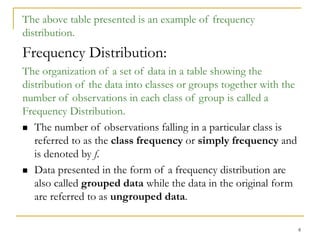
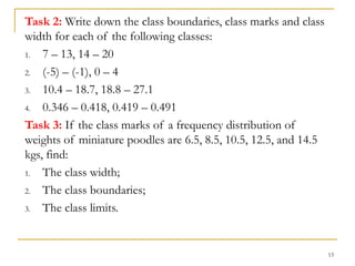
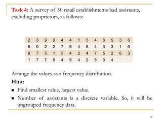
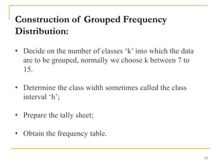
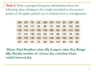
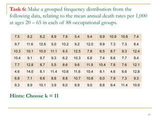
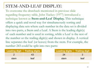
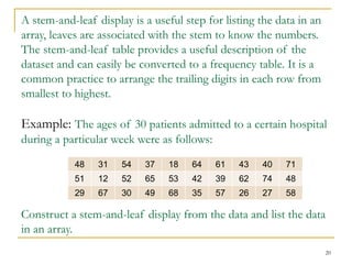
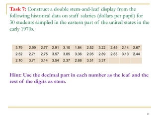
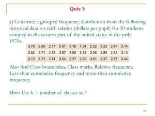
1
Presentation of Data
LECTURE #05 and 06
2
Introduction:
 Once data has been collected, it must be
classified and organized in such a way that it
becomes easily readable and interpretable,
i.e., converted to information.
 Before the calculation of descriptive statistics,
it is sometimes a good idea to present data as
tables, charts, diagrams or graphs.
 Most people find ‘pictures’ much more helpful
than ‘numbers’ in the sense that, in their
opinion, they present data more meaningfully.
3
“In this course, we will consider the various possible types of
presentation of data and justification for their use in given
situations”
4
Tabular Form:
This type of information occurs as individual observations,
usually as a table or array of disorderly values. These
observations are to be firstly arranged in some order (ascending
or descending if they are numerical) or simply grouped together
in the form of a frequency table before proper presentation on
diagrams is possible.
Arrays:
An array is a matrix of rows and columns of numbers which
have been arranged in some order (preferably ascending). It is
probably the most primitive way of tabulating information but
can be very useful if it is small in size. Some important statistics
can immediately be located by mere inspection.
5
Without any calculations, one can easily find the
1. Minimum observation
2. Maximum observation
3. Number of observations, n
Example:
we can easily verify the following:
what would be the array form of data=?
minimum value = ? maximum value = ?
number of observations = ?
24 16 23 29 49
7 18 23 33 51
8 19 2 40 54
11 19 26 44 63
15 19 27 47 68
6
Array form:
minimum value = 2
maximum value = 68
number of observations = n = 25
2 7 8 11 15
16 18 19 19 19
23 23 24 26 27
29 33 40 44 47
49 51 54 63 68
7
Simple Tables:
A table is slightly more complex than an array since it needs a heading and the
names of the variables involved. We can also use symbols to represent the
variables at times, provided they are sufficiently explicit for the reader.
Optionally, the table may also include totals or percentages (relative figures).
Example:
Distribution of Ages of FC students (males)
Age of Student Frequency
19 14
20 23
21 134
22 149
23 71
24 9
Total 400
8
The above table presented is an example of frequency
distribution.
Frequency Distribution:
The organization of a set of data in a table showing the
distribution of the data into classes or groups together with the
number of observations in each class of group is called a
Frequency Distribution.
 The number of observations falling in a particular class is
referred to as the class frequency or simply frequency and
is denoted by f.
 Data presented in the form of a frequency distribution are
also called grouped data while the data in the original form
are referred to as ungrouped data.
9
 The purpose of the frequency distribution is to produce a
meaningful pattern for the overall distribution of the data
from which conclusions can be drawn.
 A fairly common frequency pattern is the rising to a peak and
then declining. In terms of its construction, each class or
group has lower- and upper-class limits, lower- and upper-
class boundaries, a class interval and a middle value.
 In which each class consists of a single value is sometimes
called a discrete or ungrouped frequency distribution.
Class Limits:
The class-limits are defined as the values of the variables which
describe the classes; the smaller value is the lower-class limit, and
the larger value is the upper-class limit.
10
 Class-limits should be well defined and there should be no
overlapping. In other words, limits should be inclusive, i.e.,
the values corresponding exactly to the lower limit, or the
upper limit be included in that class.
 The class-limits are therefore selected in such a way that they
have the same number of significant places as the recorded
values. e.g., the data are recorded to the nearest integers, then
class limits are may be : 10 – 14, 15 – 19, 20 – 24, etc. Also,
e.g., the data are recorded to the nearest tenth of an integer,
then class limits are may be : 10.0 – 14.9, 15.0 – 19.9, 20.0 –
24.9, etc.
 Sometimes a class has either no lower class-limit or no upper
class-limit. Such a class is called an open-end class. But they
should be avoided as they are a hindrance in performing
certain calculations.
11
Class Boundaries:
The class-boundaries are the precise number which separate one
class from another. The selection of these numbers removes the
difficulty, if any, in knowing the class to which a particular value
should be assigned. A class boundary is located midway between
the upper limit of a class and the lower limit of the next higher
class.
E.g., 9.5 – 14.5, 14.5 – 19.5, 19.5 – 24.5 etc. or 9.95 – 14.95,
14.95 – 19.95, 19.95 – 24.95 etc.
Class Mark:
A class-Mark, also called class midpoint, is that number which
divides each class into two parts. It is obtained by dividing the
sum of the lower and upper limits of a class, or the sum of the
12
lower and upper boundaries of the class by 2.
Class Width or Interval:
The class-width or interval of a class is equal to the difference
between the class boundaries. It may also be obtained by finding
the difference either between two successive lower-class limits,
or between two successive class marks.
Task 1: Write down the class boundaries, class marks and class
intervals for each of the following classes:
1. 4 – 9, 10 – 15
2. 2.1 – 2.4, 2.5 – 2.8
3. -3 – 3, 4 – 10
4. 8, 12, 16
13
Task 2: Write down the class boundaries, class marks and class
width for each of the following classes:
1. 7 – 13, 14 – 20
2. (-5) – (-1), 0 – 4
3. 10.4 – 18.7, 18.8 – 27.1
4. 0.346 – 0.418, 0.419 – 0.491
Task 3: If the class marks of a frequency distribution of
weights of miniature poodles are 6.5, 8.5, 10.5, 12.5, and 14.5
kgs, find:
1. The class width;
2. The class boundaries;
3. The class limits.
14
Task 4: A survey of 50 retail establishments had assistants,
excluding proprietors, as follows:
Arrange the values as a frequency distribution.
Hint:
 Find smallest value, largest value.
 Number of assistants is a discrete variable. So, it will be
ungrouped frequency data.
2 3 9 0 4 4 1 5 4 8 5 3 6
6 0 2 2 7 6 4 8 4 3 3 1 0
8 7 5 1 3 4 2 4 7 5 2 6 3
1 7 7 5 4 6 4 2 5 3 4
15
Construction of Grouped Frequency
Distribution:
• Decide on the number of classes ‘k’ into which the data
are to be grouped, normally we choose k between 7 to
15.
• Determine the class width sometimes called the class
interval ‘h’;
• Prepare the tally sheet;
• Obtain the frequency table.
16
Task 5: Make a grouped frequency distribution from the
following data, relating to the weight recorded to the nearest
grams of 60 apples picked out at random from a consignment.
Hints: Find Smallest value (S), Largest value (L), Range
(R), Decide number of classes (k), calculate Class
width/interval (h).
106 107 76 82 109 107 115 93 187 95
123 125 111 92 86 70 126 68 130 129
139 119 115 128 100 186 84 99 113 204
111 141 136 123 90 115 98 110 78 185
162 178 140 152 173 146 158 194 148 90
107 181 131 75 184 104 110 80 118 82
17
Task 6: Make a grouped frequency distribution from the
following data, relating to the mean annual death rates per 1,000
at ages 20 – 65 in each of 88 occupational groups.
Hints: Choose k = 11
7.5 8.2 6.2 8.9 7.8 5.4 9.4 9.9 10.9 10.8 7.4
9.7 11.6 12.6 5.0 10.2 9.2 12.0 9.9 7.3 7.3 8.4
10.3 10.1 10.0 11.1 6.5 12.5 7.8 6.5 8.7 9.3 12.4
10.4 9.1 9.7 9.3 6.2 10.3 6.6 7.4 8.6 7.7 9.4
7.7 12.8 8.7 5.5 8.6 9.6 11.9 10.4 7.8 7.6 12.1
4.6 14.0 8.1 11.4 10.6 11.6 10.4 8.1 4.6 6.6 12.8
6.8 7.1 6.6 8.8 8.8 10.7 10.8 6.0 7.9 7.3 9.3
9.3 8.9 10.1 3.9 6.0 6.9 9.0 8.8 9.4 11.4 10.9
18
A clear disadvantage of using frequency table is that the identity
of individual observations is lost in grouping process
So here we introduce the concept of
Stem-and-Leaf Display
19
STEM-AND-LEAF DISPLAY:
To overcome the drawback mentioned in previous slide
regarding frequency table, John Tuckey (1977) introduced a
technique known as Stem-and-Leaf Display. This technique
offers a quick and novel way for simultaneously sorting and
displaying data sets where each number in the data set is divided
into two parts, a Stem and a Leaf. A Stem is the leading digit(s)
of each number and is used in sorting, while a Leaf is the rest of
the number or the trailing digit(s) and shown in display. A vertical
line separates the leaf (or leaves) from the stem. For example, the
number 243 could be split into two parts:
Leading digit Trailing digits
2 43
stem leaf
Leading digits Trailing digit
24 3
stem leaf
20
A stem-and-leaf display is a useful step for listing the data in an
array, leaves are associated with the stem to know the numbers.
The stem-and-leaf table provides a useful description of the
dataset and can easily be converted to a frequency table. It is a
common practice to arrange the trailing digits in each row from
smallest to highest.
Example: The ages of 30 patients admitted to a certain hospital
during a particular week were as follows:
Construct a stem-and-leaf display from the data and list the data
in an array.
48 31 54 37 18 64 61 43 40 71
51 12 52 65 53 42 39 62 74 48
29 67 30 49 68 35 57 26 27 58
21
Task 7: Construct a double stem-and-leaf display from the
following historical data on staff salaries (dollars per pupil) for
30 students sampled in the eastern part of the united states in the
early 1970s.
Hint: Use the decimal part in each number as the leaf and the
rest of the digits as stem.
3.79 2.99 2.77 2.91 3.10 1.84 2.52 3.22 2.45 2.14 2.67
2.52 2.71 2.75 3.57 3.85 3.36 2.05 2.89 2.83 3.13 2.44
2.10 3.71 3.14 3.54 2.37 2.68 3.51 3.37
22
Quiz 1:
a) Construct a grouped frequency distribution from the following
historical data on staff salaries (dollars per pupil) for 30 students
sampled in the eastern part of the united states in the early
1970s.
Also find Class boundaries, Class marks, Relative frequency,
Less-than cumulative frequency and more-than cumulative
frequency.
Hint: Use k = number of classes as 7
3.79 2.99 2.77 2.91 3.10 1.84 2.52 3.22 2.45 2.14
2.52 2.71 2.75 3.57 3.85 3.36 2.05 2.89 2.83 3.13
2.10 3.71 3.14 3.54 2.37 2.68 3.51 3.37 2.67 2.44

1) Chapter#02 Presentation of Data.ppt

  • 1.
  • 2.
    2 Introduction:  Once datahas been collected, it must be classified and organized in such a way that it becomes easily readable and interpretable, i.e., converted to information.  Before the calculation of descriptive statistics, it is sometimes a good idea to present data as tables, charts, diagrams or graphs.  Most people find ‘pictures’ much more helpful than ‘numbers’ in the sense that, in their opinion, they present data more meaningfully.
  • 3.
    3 “In this course,we will consider the various possible types of presentation of data and justification for their use in given situations”
  • 4.
    4 Tabular Form: This typeof information occurs as individual observations, usually as a table or array of disorderly values. These observations are to be firstly arranged in some order (ascending or descending if they are numerical) or simply grouped together in the form of a frequency table before proper presentation on diagrams is possible. Arrays: An array is a matrix of rows and columns of numbers which have been arranged in some order (preferably ascending). It is probably the most primitive way of tabulating information but can be very useful if it is small in size. Some important statistics can immediately be located by mere inspection.
  • 5.
    5 Without any calculations,one can easily find the 1. Minimum observation 2. Maximum observation 3. Number of observations, n Example: we can easily verify the following: what would be the array form of data=? minimum value = ? maximum value = ? number of observations = ? 24 16 23 29 49 7 18 23 33 51 8 19 2 40 54 11 19 26 44 63 15 19 27 47 68
  • 6.
    6 Array form: minimum value= 2 maximum value = 68 number of observations = n = 25 2 7 8 11 15 16 18 19 19 19 23 23 24 26 27 29 33 40 44 47 49 51 54 63 68
  • 7.
    7 Simple Tables: A tableis slightly more complex than an array since it needs a heading and the names of the variables involved. We can also use symbols to represent the variables at times, provided they are sufficiently explicit for the reader. Optionally, the table may also include totals or percentages (relative figures). Example: Distribution of Ages of FC students (males) Age of Student Frequency 19 14 20 23 21 134 22 149 23 71 24 9 Total 400
  • 8.
    8 The above tablepresented is an example of frequency distribution. Frequency Distribution: The organization of a set of data in a table showing the distribution of the data into classes or groups together with the number of observations in each class of group is called a Frequency Distribution.  The number of observations falling in a particular class is referred to as the class frequency or simply frequency and is denoted by f.  Data presented in the form of a frequency distribution are also called grouped data while the data in the original form are referred to as ungrouped data.
  • 9.
    9  The purposeof the frequency distribution is to produce a meaningful pattern for the overall distribution of the data from which conclusions can be drawn.  A fairly common frequency pattern is the rising to a peak and then declining. In terms of its construction, each class or group has lower- and upper-class limits, lower- and upper- class boundaries, a class interval and a middle value.  In which each class consists of a single value is sometimes called a discrete or ungrouped frequency distribution. Class Limits: The class-limits are defined as the values of the variables which describe the classes; the smaller value is the lower-class limit, and the larger value is the upper-class limit.
  • 10.
    10  Class-limits shouldbe well defined and there should be no overlapping. In other words, limits should be inclusive, i.e., the values corresponding exactly to the lower limit, or the upper limit be included in that class.  The class-limits are therefore selected in such a way that they have the same number of significant places as the recorded values. e.g., the data are recorded to the nearest integers, then class limits are may be : 10 – 14, 15 – 19, 20 – 24, etc. Also, e.g., the data are recorded to the nearest tenth of an integer, then class limits are may be : 10.0 – 14.9, 15.0 – 19.9, 20.0 – 24.9, etc.  Sometimes a class has either no lower class-limit or no upper class-limit. Such a class is called an open-end class. But they should be avoided as they are a hindrance in performing certain calculations.
  • 11.
    11 Class Boundaries: The class-boundariesare the precise number which separate one class from another. The selection of these numbers removes the difficulty, if any, in knowing the class to which a particular value should be assigned. A class boundary is located midway between the upper limit of a class and the lower limit of the next higher class. E.g., 9.5 – 14.5, 14.5 – 19.5, 19.5 – 24.5 etc. or 9.95 – 14.95, 14.95 – 19.95, 19.95 – 24.95 etc. Class Mark: A class-Mark, also called class midpoint, is that number which divides each class into two parts. It is obtained by dividing the sum of the lower and upper limits of a class, or the sum of the
  • 12.
    12 lower and upperboundaries of the class by 2. Class Width or Interval: The class-width or interval of a class is equal to the difference between the class boundaries. It may also be obtained by finding the difference either between two successive lower-class limits, or between two successive class marks. Task 1: Write down the class boundaries, class marks and class intervals for each of the following classes: 1. 4 – 9, 10 – 15 2. 2.1 – 2.4, 2.5 – 2.8 3. -3 – 3, 4 – 10 4. 8, 12, 16
  • 13.
    13 Task 2: Writedown the class boundaries, class marks and class width for each of the following classes: 1. 7 – 13, 14 – 20 2. (-5) – (-1), 0 – 4 3. 10.4 – 18.7, 18.8 – 27.1 4. 0.346 – 0.418, 0.419 – 0.491 Task 3: If the class marks of a frequency distribution of weights of miniature poodles are 6.5, 8.5, 10.5, 12.5, and 14.5 kgs, find: 1. The class width; 2. The class boundaries; 3. The class limits.
  • 14.
    14 Task 4: Asurvey of 50 retail establishments had assistants, excluding proprietors, as follows: Arrange the values as a frequency distribution. Hint:  Find smallest value, largest value.  Number of assistants is a discrete variable. So, it will be ungrouped frequency data. 2 3 9 0 4 4 1 5 4 8 5 3 6 6 0 2 2 7 6 4 8 4 3 3 1 0 8 7 5 1 3 4 2 4 7 5 2 6 3 1 7 7 5 4 6 4 2 5 3 4
  • 15.
    15 Construction of GroupedFrequency Distribution: • Decide on the number of classes ‘k’ into which the data are to be grouped, normally we choose k between 7 to 15. • Determine the class width sometimes called the class interval ‘h’; • Prepare the tally sheet; • Obtain the frequency table.
  • 16.
    16 Task 5: Makea grouped frequency distribution from the following data, relating to the weight recorded to the nearest grams of 60 apples picked out at random from a consignment. Hints: Find Smallest value (S), Largest value (L), Range (R), Decide number of classes (k), calculate Class width/interval (h). 106 107 76 82 109 107 115 93 187 95 123 125 111 92 86 70 126 68 130 129 139 119 115 128 100 186 84 99 113 204 111 141 136 123 90 115 98 110 78 185 162 178 140 152 173 146 158 194 148 90 107 181 131 75 184 104 110 80 118 82
  • 17.
    17 Task 6: Makea grouped frequency distribution from the following data, relating to the mean annual death rates per 1,000 at ages 20 – 65 in each of 88 occupational groups. Hints: Choose k = 11 7.5 8.2 6.2 8.9 7.8 5.4 9.4 9.9 10.9 10.8 7.4 9.7 11.6 12.6 5.0 10.2 9.2 12.0 9.9 7.3 7.3 8.4 10.3 10.1 10.0 11.1 6.5 12.5 7.8 6.5 8.7 9.3 12.4 10.4 9.1 9.7 9.3 6.2 10.3 6.6 7.4 8.6 7.7 9.4 7.7 12.8 8.7 5.5 8.6 9.6 11.9 10.4 7.8 7.6 12.1 4.6 14.0 8.1 11.4 10.6 11.6 10.4 8.1 4.6 6.6 12.8 6.8 7.1 6.6 8.8 8.8 10.7 10.8 6.0 7.9 7.3 9.3 9.3 8.9 10.1 3.9 6.0 6.9 9.0 8.8 9.4 11.4 10.9
  • 18.
    18 A clear disadvantageof using frequency table is that the identity of individual observations is lost in grouping process So here we introduce the concept of Stem-and-Leaf Display
  • 19.
    19 STEM-AND-LEAF DISPLAY: To overcomethe drawback mentioned in previous slide regarding frequency table, John Tuckey (1977) introduced a technique known as Stem-and-Leaf Display. This technique offers a quick and novel way for simultaneously sorting and displaying data sets where each number in the data set is divided into two parts, a Stem and a Leaf. A Stem is the leading digit(s) of each number and is used in sorting, while a Leaf is the rest of the number or the trailing digit(s) and shown in display. A vertical line separates the leaf (or leaves) from the stem. For example, the number 243 could be split into two parts: Leading digit Trailing digits 2 43 stem leaf Leading digits Trailing digit 24 3 stem leaf
  • 20.
    20 A stem-and-leaf displayis a useful step for listing the data in an array, leaves are associated with the stem to know the numbers. The stem-and-leaf table provides a useful description of the dataset and can easily be converted to a frequency table. It is a common practice to arrange the trailing digits in each row from smallest to highest. Example: The ages of 30 patients admitted to a certain hospital during a particular week were as follows: Construct a stem-and-leaf display from the data and list the data in an array. 48 31 54 37 18 64 61 43 40 71 51 12 52 65 53 42 39 62 74 48 29 67 30 49 68 35 57 26 27 58
  • 21.
    21 Task 7: Constructa double stem-and-leaf display from the following historical data on staff salaries (dollars per pupil) for 30 students sampled in the eastern part of the united states in the early 1970s. Hint: Use the decimal part in each number as the leaf and the rest of the digits as stem. 3.79 2.99 2.77 2.91 3.10 1.84 2.52 3.22 2.45 2.14 2.67 2.52 2.71 2.75 3.57 3.85 3.36 2.05 2.89 2.83 3.13 2.44 2.10 3.71 3.14 3.54 2.37 2.68 3.51 3.37
  • 22.
    22 Quiz 1: a) Constructa grouped frequency distribution from the following historical data on staff salaries (dollars per pupil) for 30 students sampled in the eastern part of the united states in the early 1970s. Also find Class boundaries, Class marks, Relative frequency, Less-than cumulative frequency and more-than cumulative frequency. Hint: Use k = number of classes as 7 3.79 2.99 2.77 2.91 3.10 1.84 2.52 3.22 2.45 2.14 2.52 2.71 2.75 3.57 3.85 3.36 2.05 2.89 2.83 3.13 2.10 3.71 3.14 3.54 2.37 2.68 3.51 3.37 2.67 2.44