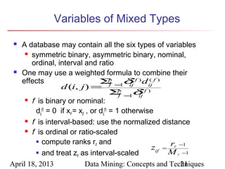
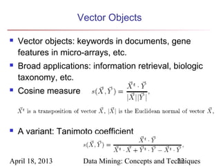
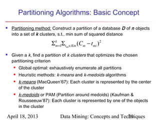
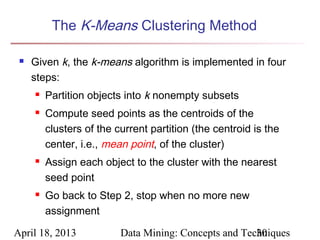
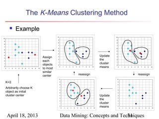
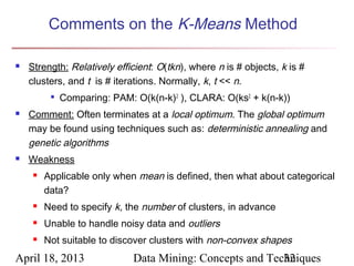
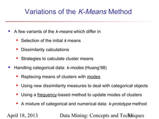
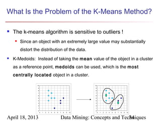
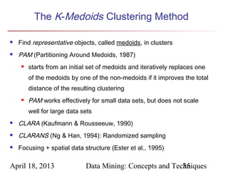
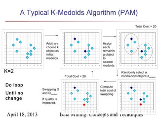
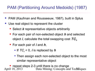
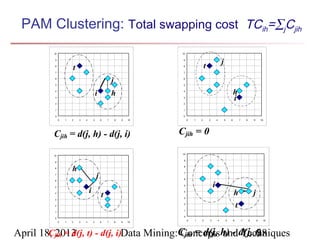
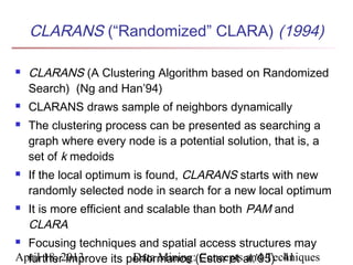
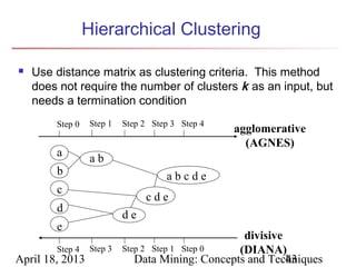
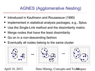
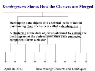
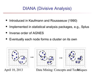
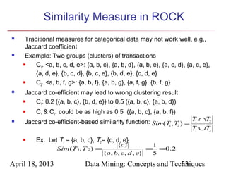
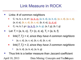
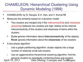
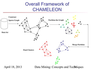
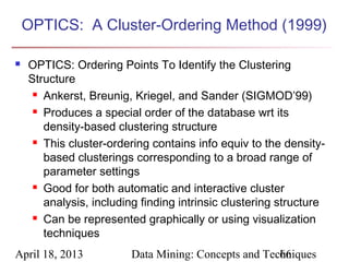
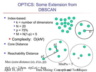
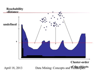
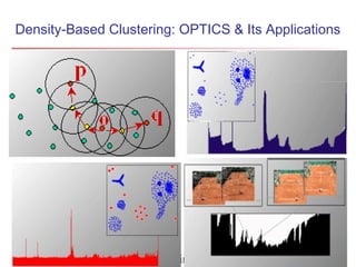
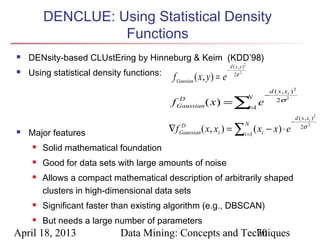
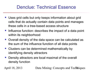
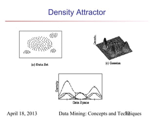
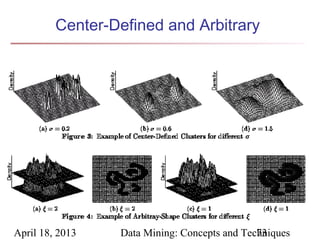
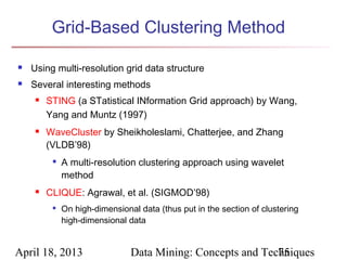
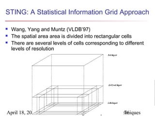
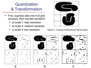
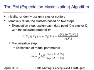
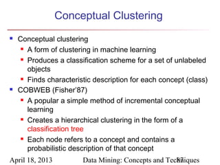
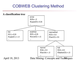
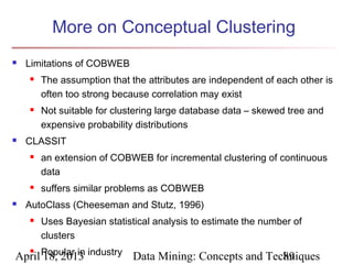
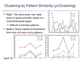
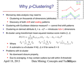
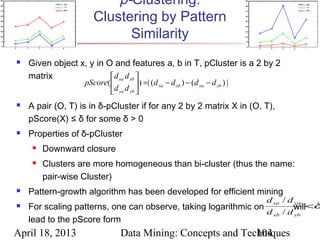
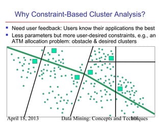
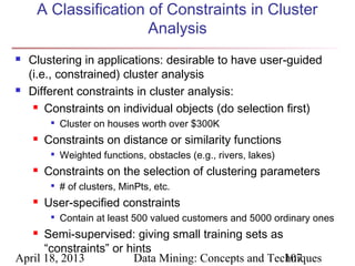
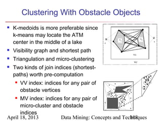
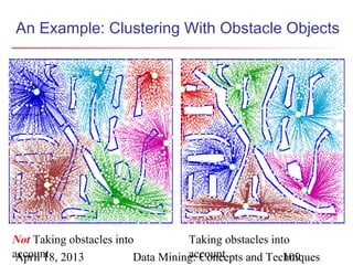
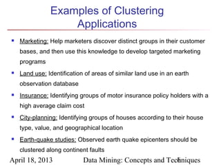
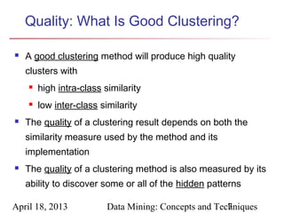
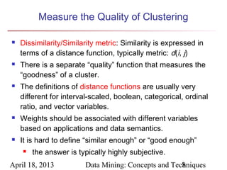
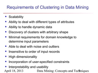
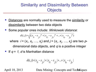
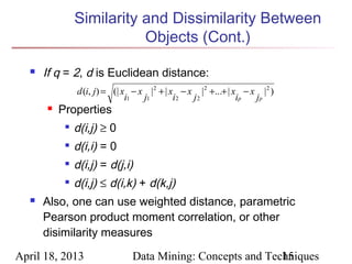
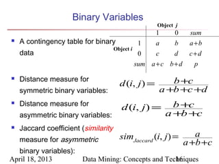
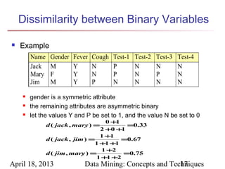
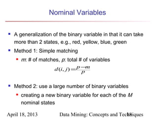
The document describes chapter 7 of the book "Data Mining: Concepts and Techniques" which covers cluster analysis. The chapter discusses what cluster analysis is, different types of data that can be analyzed, major clustering methods like partitioning, hierarchical, and density-based methods. It also covers measuring cluster quality, requirements for clustering in data mining, and how to calculate similarity and dissimilarity between data objects.
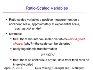
![Ordinal Variables
An ordinal variable can be discrete or continuous
Order is important, e.g., rank
Can be treated like interval-scaled
rif ∈ 1,..., M f }
{
replace xif by their rank
map the range of each variable onto [0, 1] by replacing
i-th object in the f-th variable by
rif − 1
zif =
Mf − 1
compute the dissimilarity using methods for interval-
scaled variables
April 18, 2013 Data Mining: Concepts and Techniques
19](https://image.slidesharecdn.com/07-130418101520-phpapp02/85/Chapter-7-Data-Mining-Concepts-and-Techniques-2nd-Ed-slides-Han-amp-Kamber-19-320.jpg)