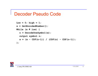
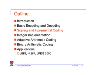
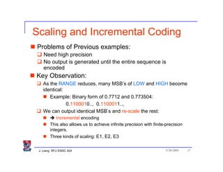
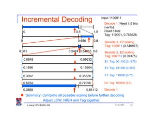
This document discusses arithmetic coding, an entropy encoding technique. It begins with an introduction comparing arithmetic coding to Huffman coding. The document then provides pseudocode for the basic encoding and decoding algorithms. It describes how scaling techniques like E1 and E2 scaling allow for incremental encoding and decoding as well as achieving infinite precision with finite-precision integers. The document outlines applications of arithmetic coding in areas like JBIG, H.264, and JPEG 2000.

1. ENSC 424 - Multimedia
Communications Engineering
Topic 6: Arithmetic Coding 1
Jie Liang
Engineering Science
Simon Fraser University
JieL@sfu.ca
J. Liang: SFU ENSC 424 9/20/2005 1

2. Outline
Introduction
Basic Encoding and Decoding
Scaling and Incremental Coding
Integer Implementation
Adaptive Arithmetic Coding
Binary Arithmetic Coding
Applications
JBIG, H.264, JPEG 2000
J. Liang: SFU ENSC 424 9/20/2005 2

3. Huffman Coding: The Retired Champion
Replacing an input symbol with a codeword
Need a probability distribution
Hard to adapt to changing statistics
Need to store the codeword table
Minimum codeword length is 1 bit
Arithmetic Coding: The Rising Star
Replace the entire input with a single floating-point
number
Does not need the probability distribution
Adaptive coding is very easy
No need to keep and send codeword table
Fractional codeword length
J. Liang: SFU ENSC 424 9/20/2005 3

4. History of Arithmetic Coding
Claude Shannon: 1916-2001
A distant relative of Thomas Edison
1932: Went to University of Michigan.
1937: Master thesis at MIT became the foundation of digital circuit design:
“The most important, and also the most famous, master's thesis of the century“
1940: PhD, MIT
1940-1956: Bell Lab (back to MIT after that)
1948: The birth of Information Theory
A mathematical theory of communication, Bell System Technical Journal.
Earliest idea of arithmetic coding
Robert Fano: 1917-
Shannon-Fano code: proved to be sub-optimal by Huffman
1952: First Information Theory class. Students included:
David Huffman: Huffman Coding
Peter Elias: Recursive implementation of arithmetic coding
Frederick Jelinek
Also Fano’s student: PhD MIT 1962 (now at Johns Hopkins)
1968: Further development of arithmetic coding
1976: Rediscovered by Pasco and Rissanen
Practical implementation: since 1980’s
Bell Lab for Sale: http://www.spectrum.ieee.org/sep05/1683
J. Liang: SFU ENSC 424 9/20/2005 4

5. Introduction
Recall table look-up decoding of Huffman code
N: alphabet size
1
L: Max codeword length
00
Divide [0, 2^L] into N intervals
One interval for one symbol
010 011
Interval size is roughly
proportional to symbol prob. 000 010 011 100
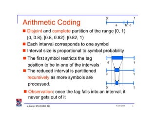
Arithmetic coding applies this idea recursively
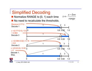
Normalizes the range [0, 2^L] to [0, 1].
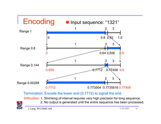
Map an input sequence to a unique tag in [0, 1).
abcd…..
dcba….. 0 1
J. Liang: SFU ENSC 424 9/20/2005 5

6. 0 1
Arithmetic Coding a b c
Disjoint and complete partition of the range [0, 1)
[0, 0.8), [0.8, 0.82), [0.82, 1)
Each interval corresponds to one symbol
Interval size is proportional to symbol probability
The first symbol restricts the tag
0 1
position to be in one of the intervals
The reduced interval is partitioned
0 1
recursively as more symbols are
processed.
0 1
Observation: once the tag falls into an interval, it
never gets out of it
J. Liang: SFU ENSC 424 9/20/2005 6

7. Some Questions to think about:
Why compression is achieved this way?
How to implement it efficiently?
How to decode the sequence?
Why is it better than Huffman code?
J. Liang: SFU ENSC 424 9/20/2005 7

8. Possible Ways to Terminate Encoding
1. Define an end of file (EOF) symbol in the
alphabet. Assign a probability for it.
0 1
a b c EOF
2. Encode the lower end of the final range.
3. If number of symbols is known to the
decoder, encode any nice number in the
final range.
J. Liang: SFU ENSC 424 9/20/2005 8

9. Example:
1 2 3
Symbol Prob.
1 0.8
0 0.8 0.82 1.0
2 0.02
Map to real line range [0, 1)
3 0.18
Order does not matter
Decoder needs to use the same order
Disjoint but complete partition:
1: [0, 0.8): 0, 0.799999…9
2: [0.8, 0.82): 0.8, 0.819999…9
3: [0.82, 1): 0.82, 0.999999…9
J. Liang: SFU ENSC 424 9/20/2005 9

10. Encoding Input sequence: “1321”
1 2 3
Range 1
0 0.8 0.82 1.0
1 2 3
Range 0.8
0 0.64 0.656 0.8
1 2 3
Range 0.144
0.656 0.7712 0.77408 0.8
1 2 3
Range 0.00288
0.7712 0.773504 0.7735616 0.77408
Termination: Encode the lower end (0.7712) to signal the end.
Difficulties: 1. Shrinking of interval requires very high precision for long sequence.
2. No output is generated until the entire sequence has been processed.
J. Liang: SFU ENSC 424 9/20/2005 10

11. Encoder Pseudo Code
Probability Mass Function
Cumulative Density Function (CDF)
0.4
For continuous distribution:
x 0.2
0.2 0.2
FX ( x) = P ( X ≤ x) =
−∞
∫ p( x)dx
1 2 3 4 X
For discrete distribution:
i 1.0
FX (i ) = P( X ≤ i ) = ∑ P( X = k )
k = −∞
CDF 0.8
0.4
Properties: 0.2
Non-decreasing
Piece-wise constant X
1 2 3 4
Each segment is closed at the lower end.
J. Liang: SFU ENSC 424 9/20/2005 11

12. Encoder Pseudo Code
low=0.0, high=1.0;
Keep track of
while (not EOF) {
LOW, HIGH, RANGE n = ReadSymbol();
Any two are RANGE = HIGH - LOW;
sufficient, e.g., HIGH = LOW + RANGE * CDF(n);
LOW and RANGE. LOW = LOW + RANGE * CDF(n-1);
}
output LOW;
Input HIGH LOW RANGE
Initial 1.0 0.0 1.0
1 0.0+1.0*0.8=0.8 0.0+1.0*0 = 0.0 0.8
3 0.0 + 0.8*1=0.8 0.0 + 0.8*0.82=0.656 0.144
2 0.656+0.144*0.82=0.77408 0.656+0.144*0.8=0.7712 0.00288
1 0.7712+0.00288*0=0.7712 0.7712+0.00288*0.8=0.773504 0.002304
J. Liang: SFU ENSC 424 9/20/2005 12

13. Decoding Receive 0.7712
1 2 3
Decode 1
0 0.8 0.82 1.0
1 2 3
Decode 3
0 0.64 0.656 0.8
1 2 3
Decode 2
0.656 0.7712 0.77408 0.8
1 2 3
Decode 1
0.7712 0.773504 0.7735616 0.77408
Drawback: need to recalculate all thresholds each time.
J. Liang: SFU ENSC 424 9/20/2005 13

14. Simplified Decoding x − low
Normalize RANGE to [0, 1) each time x←
range
No need to recalculate the thresholds.
Receive 0.7712 1 2 3
Decode 1
x =(0.7712-0) / 0.8 0 0.8 0.82 1.0
= 0.964
1 2 3
Decode 3
0 0.8 0.82 1.0
x =(0.964-0.82) / 0.18
= 0.8 1 2 3
Decode 2
x =(0.8-0.8) / 0.02 0 0.8 0.82 1.0
=0
Decode 1.
1 2 3
Stop.
0 0.8 0.82 1.0
J. Liang: SFU ENSC 424 9/20/2005 14

15. Decoder Pseudo Code
Low = 0; high = 1;
x = GetEncodedNumber();
While (x ≠ low) {
n = DecodeOneSymbol(x);
output symbol n;
x = (x - CDF(n-1)) / (CDF(n) - CDF(n-1));
};
J. Liang: SFU ENSC 424 9/20/2005 15

16. Outline
Introduction
Basic Encoding and Decoding
Scaling and Incremental Coding
Integer Implementation
Adaptive Arithmetic Coding
Binary Arithmetic Coding
Applications
JBIG, H.264, JPEG 2000
J. Liang: SFU ENSC 424 9/20/2005 16

17. Scaling and Incremental Coding
Problems of Previous examples:
Need high precision
No output is generated until the entire sequence is
encoded
Key Observation:
As the RANGE reduces, many MSB’s of LOW and HIGH become
identical:
Example: Binary form of 0.7712 and 0.773504:
0.1100010.., 0.1100011..,
We can output identical MSB’s and re-scale the rest:
Incremental encoding
This also allows us to achieve infinite precision with finite-precision
integers.
Three kinds of scaling: E1, E2, E3
J. Liang: SFU ENSC 424 9/20/2005 17

18. E1 and E2 Scaling
E1: [LOW HIGH) in [0, 0.5) 0 0.5 1.0
LOW: 0.0xxxxxxx (binary),
HIGH: 0.0xxxxxxx.
0 0.5 1.0
Output 0, then shift left by 1 bit
[0, 0.5) [0, 1): E1(x) = 2 x
E2: [LOW HIGH) in [0.5, 1) 0 0.5 1.0
LOW: 0.1xxxxxxx,
HIGH: 0.1xxxxxxx.
0 0.5 1.0
Output 1, subtract 0.5,
shift left by 1 bit
[0.5, 1) [0, 1): E2(x) = 2(x - 0.5)
J. Liang: SFU ENSC 424 9/20/2005 18

19. Encoding with E1 and E2 Symbol
1
Prob.
0.8
Input 1
2 0.02
0 0.8 1.0
3 0.18
Input 3
0 0.656 0.8 E2: Output 1
Input 2 2(x – 0.5)
0.312 0.5424 0.54816 0.6 E2: Output 1
0.0848 0.09632
E1: 2x, Output 0
0.1696 0.19264 E1: Output 0
0.3392 0.38528 E1: Output 0
0.6784 0.77056 E2: Output 1
Input 1
Encode any value
0.3568 0.54112 in the tag, e.g., 0.5
Output 1
0.3568 0.504256 All outputs: 1100011
J. Liang: SFU ENSC 424 9/20/2005 19

20. To verify
LOW = 0.5424 (0.10001010... in binary),
HIGH = 0.54816 (0.10001100... in binary).
So we can send out 10001 (0.53125)
Equivalent to E2 E1 E1 E1 E2
After left shift by 5 bits:
LOW = (0.5424 – 0.53125) x 32 = 0.3568
HIGH = (0.54816 – 0.53125) x 32 = 0.54112
Same as the result in the last page.
J. Liang: SFU ENSC 424 9/20/2005 20

21. Symbol Prob.
Note: Complete all possible scaling before
1 0.8
encoding the next symbol 2 0.02
3 0.18
Comparison with Huffman
Input Symbol 1 does not cause any output
Input Symbol 3 generates 1 bit
Input Symbol 2 generates 5 bits
Symbols with larger probabilities generates less
number of bits.
Sometimes no bit is generated at all
Advantage over Huffman coding
Large probabilities are desired in arithmetic coding
Can use context-adaptive method to create larger probability
and to improve compression ratio.
J. Liang: SFU ENSC 424 9/20/2005 21

22. Incremental Decoding Input 1100011
Decode 1: Need ≥ 5 bits
(verify)
0 0.8 1.0 Read 6 bits:
Tag: 110001, 0.765625
0 0.656 0.8 Decode 3, E2 scaling
Tag: 100011 (0.546875)
0.312 0.5424 0.54816 0.6 Decode 2, E2 scaling
Tag: 000110 (0.09375)
0.0848 0.09632
E1: Tag: 001100 (0.1875)
0.1696 0.19264 E1: Tag: 011000 (0.375)
0.3392 0.38528 E1: Tag: 110000 (0.75)
0.6784 0.77056 E2: Tag: 100000 (0.5)
0.3568 0.54112 Decode 1
Summary: Complete all possible scaling before further decoding
Adjust LOW, HIGH and Tag together.
J. Liang: SFU ENSC 424 9/20/2005 22

23. Summary
Introduction
Encoding and Decoding
Scaling and Incremental Coding
E1, E2
Next:
Integer Implementation
E3 scaling
Adaptive Arithmetic Coding
Binary Arithmetic Coding
Applications
JBIG, H.264, JPEG 2000
J. Liang: SFU ENSC 424 9/20/2005 23