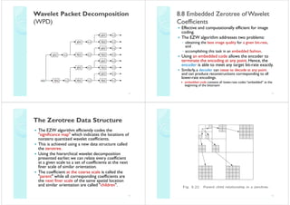
The document discusses lossy compression techniques. It begins by explaining that lossy compression algorithms compress data by discarding some information, yielding much higher compression ratios than lossless compression but resulting in distorted approximations of the original data. It then covers various lossy compression methods including quantization, transform coding using the discrete cosine transform (DCT), wavelet-based coding using the discrete wavelet transform (DWT), and techniques like vector quantization (VQ) and the Karhunen-Loeve transform (KLT) that aim to decorrelate signal components before quantization. Key aspects like rate-distortion theory, various distortion measures, and algorithms for quantization are also described.

1. Chapter 8 Lossy Compression
8.1 Introduction
81
Algorithms
8.1
8 1 Introduction Lossless compression algorithms do not
8.2 Distortion Measures deliver compression ratios that are high
8.3
8 3 The Rate-Distortion Theory
Rate Distortion
enough. Hence, most multimedia
8.4 Quantization
compression algorithms are lossy.
p g y
8.5
8 5 Transform Coding
8.6 Wavelet-Based Coding What is lossy compression ?
8.7 W l t P k t
8 7 Wavelet Packets ◦ The compressed data is not the same as the
8.8 Embedded Zerotree of Wavelet Coefficients original data, but a close approximation of it.
8.9 S Partitioning i Hierarchical T
8 9 Set P i i i in Hi hi l Trees (SPIHT) ◦ Yi ld a much hi h compression ratio than
Yields h higher i i h
8.10 Further Exploration that of loss-less compression.
1 2
8.2 Distortion Measures
82 8.3 The Rate-Distortion Theory
83 Rate-
The three most commonly used distortion measures
in image compression are: Provides a framework for the study of
◦ mean square error (MSE) σ 2, tradeoffs between Rate and Distortion.
where xn yn and N are the input data sequence
xn, yn,and sequence,
reconstructed data sequence, and length of the data
sequence respectively.
◦ signal to noise ratio (S ) in decibel units (dB),
(SNR), ( )
◦ peak signal to noise ratio (PSNR),
3 4

2. 8.4 Quantization
84 Uniform Scalar Quantization
Reduce the number of distinct output A uniform scalar quantizer partitions the domain
of input values into equally spaced intervals,
values to a much smaller set, via except p
p possibly at the two outer intervals.
y
quantization. ◦ The output or reconstruction value corresponding to
each interval is taken to be the midpoint of the
Main source of the "loss" in lossyy interval.
i l
compression. ◦ The length of each interval is referred to as the step
Three diff
Th different f
t forms of quantization.
f ti ti size,
size denoted by the symbol ∆ ∆.
Two types of uniform scalar quantizers:
◦ Uniform: midrise and midtread quantizers.
◦ Midrise quantizers have even number of output levels
levels.
◦ Nonuniform: companded quantizer. ◦ Midtread quantizers have odd number of output
◦ Vector Quantization.
Q levels, including zero as one of them (see Fig. 8.2).
5 6
For the special case where ∆ = 1, we can
1
simply compute the output values for these
q
quantizers as:
Performance of an M level quantizer. Let B =
{b0,b1,...,bM }be the set of decision
boundaries and Y = { 1,y2,. ..,yM } the set of
{y }be
reconstruction or output values.
Suppose the input is uniformly di ib d i
S h i i if l distributed in
the interval [−Xmax, Xmax]. The rate of the
quantizer is:
7 8

3. Quantization Error of Uniformly
Distributed Source
Granular distortion: quantization error caused by the quantizer for
q y q
bounded input.
To get an overall figure for granular distortion, notice that decision
boundaries bi for a midrise quantizer are [(i − 1)∆, i∆], i =1..M/2,
covering positive data X ( d another h lf for negative X values).
i ii d (and h half f i l )
Output values yi are the midpoints i∆ − ∆/2, i =1..M/2, again just
considering the positive data. The total distortion is twice the sum
over the positive data or
data,
where we divide by the range of X to normalize to a value of at
most 1.
Since the reconstruction values yi are the midpoints of each
interval, the quantization error must lie within the values. For a
uniformly distributed source, the graph of quantization error is
shown in Fig. 8 3
Fig 8.3.
9 10
Therefore,
Therefore the average squared error is Signal variance is , so
the same as the variance of the if the quantizer is n bits, M=2n, then from
quantization error calculated f
l l d from just Eq. (8.2) we have
the interval [0, Δ] with error values in
.
The error value at x is e(x) = x – Δ/2 so
Δ/2,
the variance of errors is given by
11 12

4. Nonuniform Scalar Quantization Minimize the total distortion by setting the
derivative of Eq. (8.12) to zero.
Two common approaches for nonuniform ◦ Differentiating with respect to yi yields the set of
quantization: Lloyd-Max quantizer and reconstruction values
companded quantizer.
Lloyd-Max quantizer
y q ◦ Th optimal reconstruction value i the weighted
The i l i l is h i h d
◦ The probability distribution fX(x), the decision centroid of the x interval.
boundaries bi and the reconstruction values yi ◦ Differentiating with respect to bi and setting the
Total distortion measure result to zero yields
◦ The decision boundary at the midpoint of two
adjacent reconstruction values
13 14
Companded Quantizer
Algorithm 8 1
8.1
LLOYD-MAX QUANTIZATION
BEGIN
Choose initial level set y0
I=0
Repeat
Compute bi using Eq. 8.14
I=I+1 Companded quantization is nonlinear
nonlinear.
Compute yi using Eq. 8.13 As shown above, a compander consists of a
Until | yi - yi-1 | < ε compressor function G a uniform quantizer
G, quantizer,
and an expander function G−1.
END
The two commonly used companders are
15
the µ-law and A-law companders. 16

5. Vector Quantization (VQ)
According to Shannon’s original work on
Shannon s
information theory, any compression system
p
performs better if it operates on vectors or
p
groups of samples rather than individual
symbols or samples.
Form vectors of input samples b simply
F f l by l
concatenating a number of consecutive
samples into a single vector
vector.
Instead of single reconstruction values as in
scalar quantization, in VQ code vectors with
quantization
n components are used. A collection of
these code vectors form the codebook.
17 18
8.5 Transform Coding
85 Spatial Frequency and DCT
The rationale behind transform coding: Spatial frequency indicates how many times
If Y is the result of a linear transform T of the input pixel values change across an image block.
vector X in such a way that the components of Y are
much less correlated then Y can be coded more
correlated, The DCT formalizes this notion with a
efficiently than X. measure of how much the image contents
If most information is accurately described by the
y y change in correspondence to the number of
first few components of a transformed vector, then
the remaining components can be coarsely quantized, cycles of a cosine wave per block.
or even set to zero, with little signal distortion. The role of the DCT is to decompose the
Discrete Cosine Transform (DCT) will be studied first. original signal into its DC and AC
In addition, we will examine the Karhunen-Loeve
Transform (KLT) which optimally d
T f hi h ti ll decorrelates th
l t the components; the role of the IDCT is to
components of the input X. reconstruct (re-compose) the signal.
19 20

6. Definition of DCT:
DCT:
Given an input function f(i j) over two
f(i,
integer variables i and j (a piece of an image),
the 2D DCT transforms it into a new
function F(u, v), with integer u and v running
over the same range as i and j.
The general definition of the transform is:
21 22
23 24

7. 25 26
27 28

8. The DCT is a linear transform
transform.
In general, a transform T (or function) is
linear, iff
T (αp + βq)= αT (p)+ βT (q)
βq) (8.21)
(8 21)
where α and β are constants, p and q are
any ffunctions, variables or constants.
bl
From the definition in Eq. 8.17 or 8.19,
q ,
this property can readily be proven for
the DCT because it uses only simple
29
arithmetic operations. 30
The Cosine Basis Functions
31 32

9. 2D Separable Basis Comparison of DCT and DFT
The 2D DCT can be separated into a sequence of The discrete cosine transform is a close counterpart
two, 1D DCT steps: to the Discrete Fourier Transform (DFT). DCT is a
transform that only involves the real part of the DFT.
For a continuous signal we define the continuous
signal,
Fourier
Because the use of digital computers requires us to
It is straightforward to see that this simple change discretize the input signal we define a DFT that
signal,
saves many arithmetic steps. The number of operates on 8 samples of the input signal {f0,f1,...,f7}
as:
iterations required is reduced from 8×8 to 8+8.
8 8 8 8.
33 34
Writing the sine and cosine terms explicitly, we have
The formulation of the DCT that allows it to use only
the cosine basis functions of the DFT is that we can
cancel out the imaginary part of the DFT by making a
symmetric copy of the original input signal.
DCT of 8 input samples corresponds to DFT of the
16 samples made up of original 8 input samples and a
symmetric copy of these, as shown in Fig. 8.10.
35 36

10. A Simple Comparison of DCT and
DFT
Table 8 1 and Fig. 8.11 show the comparison
8.1 Fig 8 11
of DCT and DFT on a ramp function, if only
the first three t
th fi t th terms are used.
d
37 38
Karhunen-
Karhunen-Loeve Transform (KLT)
(KLT) Our goal is to find a transform T such that the
g
components of the output Y are uncorrelated,
i.e ,if t ≠s. Thus, the autocorrelation
The Karhunen-Loeve transform is a matrix of Y takes on the form of a positive diagonal
matrix.
reversible linear transform that exploits the
Since any autocorrelation matrix is symmetric and
statistical properties of the vector non-negative d fi i there are k orthogonal
i definite, h h l
representation. eigenvectors u1,u2,...,uk and k corresponding real and
nonnegative eigenvalues λ1 ≥ λ2 ≥ ···≥λk ≥0.
g g
It optimally decorrelates the input signal
signal.
If we define the Karhunen-Loeve transform as
To understand the optimality of the KLT,
consider the autocorrelation matrix RX of
the input vector X defined as Then, the autocorrelation matrix of Y becomes
39 40

11. KLT Example
To illustrate the mechanics of the KLT KLT, The eigenvalues of RX are λ1=6 1963
=6.1963,
consider the four 3D input vectors x1 =(4, λ2=0.2147, and λ3=0.0264. The
4, 5), x2 =(3, 2, 5), x3 =(5, 7, 6), and x4 =(6, corresponding eigenvectors are
)
7, 7).
41 42
8.6 Wavelet-Based Coding
8 6 Wavelet-
Subtracting the mean vector from each input vector and
g p The objective of the wavelet transform is to
apply the KLT decompose the input signal into components that are
easier to deal with, have special interpretations, or
have some components that can be thresholded away away,
for compression purposes.
We want to be able to at least approximately
reconstruct the original signal given these
h i i l i l i h
Since the rows of T are orthonormal vectors, the inverse components.
transform is just the transpose: T−1= TT ,and The basis functions of the wavelet transform are
localized in both time and frequency.
There are two types of wavelet transforms: the
In
I general, after the KLT most of the "energy" of the
l f h f h " " f h continuous wavelet t
ti l t transform (CWT) and th
f d the
transform coefficients are concentrated within the first few discrete wavelet transform (DWT).
components. This is the "energy compaction" property of the
KLT.
KLT
43 44

12. The Continuous Wavelet Transform
The continuous wavelet transform (CWT)
of f L2(R)at time u and scale s is defined
as:
The inverse of the continuous wavelet
transform is:
t f i
45 46
Multiresolution Analysis in the
The Discrete Wavelet Transform
Wavelet Domain
Discrete wavelets are again formed from a Multiresolution analysis provides the tool to adapt
mother wavelet, but with scale and shift in signal resolution to only relevant details for a
particular task.
discrete steps.
p
The approximation component is then recursively
The DWT makes the connection between decomposed into approximation and detail at
wavelets in the continuous time domain and successively coarser scales.
"filter banks"
"f l b k " in the discrete time domain in
h d d Wavelet functions ψ(t) are used to characterize detail
a multiresolution analysis framework. information. The averaging (approximation)
information is formally determined by a kind of dual
It is possible to show that the dil t d and
i ibl t h th t th dilated d to the mother wavelet, called the "scaling function"
translated family of wavelets ψ φ(t).
Wavelets
W l t are set up such that the approximation at
t h th t th i ti t
resolution 2−j contains all the necessary information
to compute an approximation at coarser resolution
form
f rm an orthonormal basis of L2(R)
rth n rmal f (R). 2−(j+1)
(j+1)
47 48

13. The scaling function must satisfy the so-called dilation
equation:
The wavelet at the coarser level is also expressible as
a sum of translated scaling functions:
The vectors h0[n] and h1[n] are called the low pass
low-pass
and high-pass analysis filters. To reconstruct the
original input, an inverse operation is needed. The
inverse filt
i filters are called synthesis filt
ll d th i filters.
49 50
Wavelet Transform Example
Suppose we are given the following input sequence.
pp g g p q Form a new sequence having length equal to that of
the original sequence by concatenating the two
sequences {xn−1,i } and {dn−1,i }. The resulting sequence
Consider h
C id the transform that replaces the original sequence
f h l h i i l is
with its pairwise average xn−1,i and difference dn−1,i defined as
follows:
This sequence has exactly the same number of
elements as the input sequence — the transform did
not increase the amount of data
data.
Since the first half of the above sequence contain
averages from the original sequence, we can view it as
g g q
The
Th averages and d ff
d differences are applied only on consecutive
l d l a coarser approximation to the original signal. The
pairs of input sequences whose first element has an even second half of this sequence can be viewed as the
index. Therefore, the number of elements in each set {xn−1,i } details or approximation errors of the first half.
pp
and {dn−1,i } i exactly half of th number of elements i th
d is tl h lf f the b f l t in the
original sequence.
51 52

14. It is easily verified that the original sequence
y g q
can be reconstructed from the transformed
sequence using the relations
This transform is the discrete Haar wavelet
transform.
53 54
55 56

15. 57 58
Biorthogonal Wavelets
For orthonormal wavelets, the forward transform
and its inverse are transposes of each other and
the analysis filters are identical to the synthesis
filters.
filters
Without orthogonality, the wavelets for analysis
and synthesis are called “biorthogonal”. The
biorthogonal .
synthesis filters are not identical to the analysis
filters. We denote them as and .
To specify a biorthogonal wavelet transform, we
require both
59 60

16. 2D Wavelet Transform
For an N by N input image, the two-dimensional
two dimensional
DWT proceeds as follows:
◦ Convolve each row of the image with h0[n] and h1[n],
discard the odd numbered columns of the resulting arrays
arrays,
and concatenate them to form a transformed row.
◦ After all rows have been transformed, convolve each
column of the result with h0[n]and h1[n] Again discard the
[n].
odd numbered rows and concatenate the result.
After the above two steps, one stage of the DWT is
complete. Th transformed i
l The f d image now contains four
i f
subbands LL, HL, LH, and HH, standing for low-low,
high-low, etc.
g
The LL subband can be further decomposed to yield
yet another level of decomposition. This process can
be continued until the desired number of
decomposition levels is reached.
61 62
2D Wavelet Transform Example
The input image is a sub-sampled version of
the image Lena. The size of the input is
16×16.
16×16 The filter used in the example is the
Antonini 9/7 filter set
63 64

17. The input image is shown in numerical
form below. Convolve the first row with both h0[n] and h1[n]
and discarding the values with odd-numbered
index. The results of these two operations are:
p
Form the transformed output row by
concatenating the resulting coefficients. The first
g g
row of the transformed image is then:
First,
First we need to compute the analysis
and synthesis high-pass filters. Continue the same process for the remaining
rows.
65 66
Apply the filters to the columns of the resulting
image.
image Apply both h0[n] and h1[n] to each column
and discard the odd indexed results:
The result after all rows have been
processed Concatenate the above results into a single column
and apply the same procedure to each of the
remaining columns.
67 68

18. This completes one stage of the discrete
wavelet transform. We can perform another
transform
stage of the DWT by applying the same
transform procedure illustrated above to the
f d ill d b h
upper left 8 × 8 DC image of I12(x, y). The
resulting two-stage transformed image is
69 70
8.7 Wavelet Packets
87 Discrete Wavelet Transform
In the usual dyadic wavelet decomposition, only
the low-pass filtered subband is recursively
decomposed and thus can be represented by a
logarithmic
l arithmic tree str ct re
structure.
A wavelet packet decomposition allows the
decomposition to be represented by any pruned
subtree of the full tree topology.
The wavelet packet decomposition is very flexible
since a best wavelet basis in the sense of some
cost metric can be found within a large library of
permissible bases
bases.
The computational requirement for wavelet
packet decomposition is relatively low as each
decomposition can be computed in the order of
NlogN using fast filter banks. 71 72

19. Wavelet Packet Decomposition 8.8 Embedded Zerotree of Wavelet
(WPD) Coefficients
Effective and computationally efficient for image
coding.
The EZW algorithm addresses two problems:
◦ obtaining the best image quality for a given bit-rate,
and
◦ accomplishing this task in an embedded fashion
fashion.
Using an embedded code allows the encoder to
terminate the encoding at any point. Hence, the
g yp
encoder is able to meet any target bit-rate exactly.
Similarly, a decoder can cease to decode at any point
and can produce reconstructions corresponding to all
lower-rate encodings.
embedded code contains all lower-rate codes “embedded” at the
beginning of the bitstream
73 74
The Zerotree Data Structure
The EZW algorithm efficiently codes the
"significance map" which indicates the locations of
nonzero quantized wavelet coefficients.
This
Th is achieved using a new data structure called
h d d ll d
the zerotree.
Using the hierarchical wavelet decomposition
presented earlier, we can relate every coefficient
at a given scale to a set of coefficients at the next
finer scale of similar orientation.
The coefficient at the coarse scale is called the
"parent" while all corresponding coefficients are
parent
the next finer scale of the same spatial location
and similar orientation are called "children".
75 76

20. Given a threshold T, a coefficient x is an element of
the zerotree if it is insignificant and all of its
descendants are insignificant as well.
The significance map is coded using the zerotree with
a four-symbol alphabet:
◦ The zerotree root: The root of the zerotree is encoded
with a special symbol indicating that the insignificance of
the coefficients at finer scales is completely predictable.
◦ Isolated zero: The coefficient is insignificant but has some
g
significant descendants.
◦ Positive significance: The coefficient is significant with a
p
positive value.
◦ Negative significance: The coefficient is significant with a
negative value.
77 78
Successive Approximation
Dominant Pass
Quantization
Motivation: Coefficients having their coordinates on the
◦ Takes advantage of the efficient encoding of the dominant list implies that they are not yet
significance map using the zerotree data structure by g
significant.
allowing it to encode more significance maps
maps.
◦ Produce an embedded code that provides a coarse- Coefficients are compared to the threshold Ti to
to-fine, multiprecision logarithmic representation of
p g p determine their significance. If a coefficient is
the scale space corresponding to the wavelet- found to be significant, its magnitude is appended
transformed image. to the subordinate list and the coefficient in the
The SAQ method sequentially applies a sequence wavelet t
l t transform array i set to 0 to enable the
f is t t t bl th
of thresholds T0,...,TN−1 to determine the possibility of the occurrence of a zerotree on
significance of each coefficient.
future dominant passes at smaller thresholds
thresholds.
A dominant list and a subordinate list are
maintained during the encoding and decoding The resulting significance map is zerotree coded.
process.
process
79 80

21. Subordinate Pass
All coefficients on the subordinate list are scanned
and their magnitude (as it is made available to the EZW Example
decoder) is refined to an additional bit of precision.
The width of the uncertainty interval for the true
magnitude of the coefficients is cut in half.
For each magnitude on the subordinate list, the
g ,
refinement can be encoded using a binary alphabet
with a "1" indicating that the true value falls in the
upper half of the uncertainty interval and a "0" 0
indicating that it falls in the lower half.
After the completion of the subordinate pass, the
magnitudes on the subordinate li t are sorted i
it d th b di t list t d in
decreasing order to the extent that the decoder can
perform the same sort.
81 82
Encoding The
Th coefficient −29 i i i ifi
ffi i 29 is insignificant, b contains a significant
but
descendant 33 in LH1. Therefore, it is coded as z.
i i ifi
Since the largest coefficient is 57 the initial
57, The coefficient 30 is also insignificant, and all its descendant
are insignificant, so it is coed as t.
threshold T0 is 32. Continuing in this manner, the dominant pass outputs the
At the beginning, the dominant list contains following symbols:
g y
the coordinates of all the coefficients. {57(p), −37(n), −29(z), 30(t), 39(p), −20(t), 17(t), 33(p), 14(t),
6(z), 10(t), 19(t), 3(t), 7(t), 8(t), 2(t), 2(t), 3(t), 12(t), −9(t),
The following is the list of coefficients visited
g 33(p), 20(t), 2(t), 4(t)}
(p), ( ), ( ), ( )}
in the order of the scan:
{57, −37, −29, 30, 39, −20, 17, 33, 14, 6, 10, 19, There are five coefficients found to be significant: 57, -37, 39,
33,
33 and another 33. Since we know that no coefficients are
33
3, 7, 8, 2, 2, 3, 12, −9, 33, 20, 2, 4}
} greater than 2T0 = 64 and the threshold used in the first
With respect to the threshold T0 = 32, it is dominant pass is 32, the uncertainty interval is thus [32, 64).
easy to see that the coefficients 57 and -37
h h ffi i d 37 The subordinate pass following the dominant pass refines the
magnitude of these coefficients by indicating whether they lie
are significant. Thus, we output a p and a n in the first half or the second half of the uncertainty interval.
to represent them them.
83 84

22. Now the dominant list contains the coordinates of all Before we move on to the second round of
the coefficients except those found to be significant dominant and subordinate passes, we need
and the subordinate list contains the values:
to set the values of the significant
g
dominant list: { 29 30 39, −20, 17, 14, 6, 10, 19, 3, 7, 8,
{−29, 30, 39 20 17 14 6 10 19 3 7 8 coefficients to 0 in the wavelet transform
2, 2, 3, 12, −9, 20, 2, 4}
subordinate list: {57, 37, 39, 33, 33}.
{ , , , , }
array so that they do not prevent the
Now, we attempt to rearrange the values in the
emergence of a new zerotree
zerotree.
subordinate list such that larger coefficients appear The new threshold for second dominant
before smaller ones with the constraint that the
ones, pass is T1 = 16 Using the same procedure as
16.
decoder is able do exactly the same. above, the dominant pass outputs the
The decoder is able to distinguish values from [32, 48)
g [ ) following symbols
g y
and [48, 64). Since 39 and 37 are not distinguishable in
the decoder, their order will not be changed.
The subordinate list is now:
85 86
The subordinate pass that follows will halve
each of the three current uncertainty Decoding
intervals [48, 64), [32, 48), and [16, 32). The Suppose we only received information from the first
pp y
subordinate pass outputs the following bits:
b d h f ll b dominant and subordinate pass.
From the symbols in D0 we can obtain the position of the
significant coefficients.
Then, using the bits decoded from S0, we can reconstruct the
value of these coefficients using the center of the uncertainty
The output of the subsequent dominant and
p q interval.
subordinate passes are shown below:
87 88

23. 8.9 Set Partitioning in Hierarchical
If the decoder received only D0, S0, D1, S1, Trees (SPIHT)
The SPIHT algorithm is an extension of the EZW
D2, and only the first 10 bits of S2, then algorithm.
the reconstruction is The SPIHT algorithm significantly improved the
performance of its predecessor by changing the way
subsets of coefficients are partitioned and how
refinement information is conveyed.
A unique property of the SPIHT bitstream is its
compactness. The resulting bitstream from the SPIHT
algorithm is so compact that passing it through an
entropy coder would only produce very marginal gain
in compression.
No d i i f
N ordering information i explicitly transmitted t
ti is li itl t itt d to
the decoder. Instead, the decoder reproduces the
execution path of the encoder and recovers the
ordering information.
f
89 90
8.10 Further Explorations
8 10
Text books:
◦ Introduction to Data Compression by Khalid Sayood
◦ Vector Quantization and Signal Compression by Allen Gersho
and Robert M. Gray
◦ Digital Image Processing by Rafael C. Gonzales and Richard E.
Woods
◦ Probability and Random Processes with Applications to Signal
Processing by Henry Stark and John W. Woods
◦ A Wavelet Tour of Signal Processing by Stephane G. Mallat
Web sites: → Link to Further Exploration for Chapter 8
8..
including:
◦ An online graphics-based demonstration of the wavelet
transform.
transform
◦ Links to documents and source code related to quantization,
Theory of Data Compression webpage, FAQ for
comp.compression, etc.
◦ A link to an excellent article Image Compression – from DCT to
Wavelets : A Review. 91