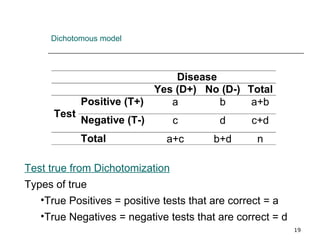
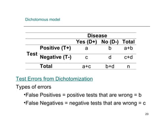
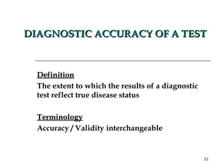
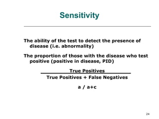
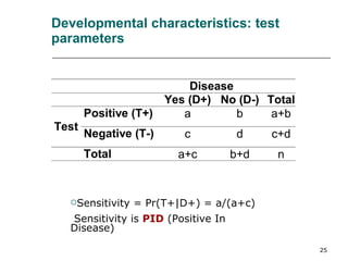
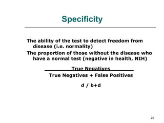
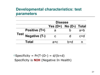
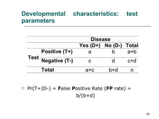
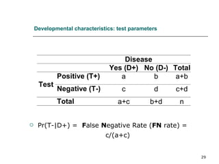
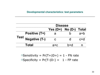
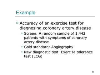
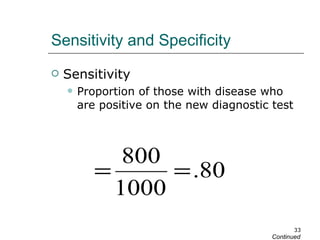
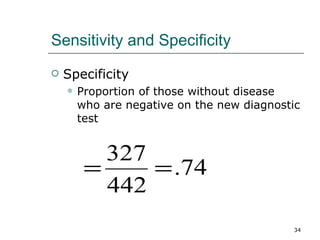
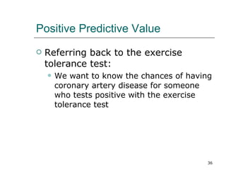
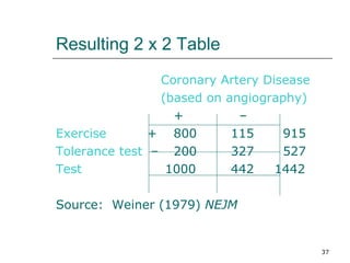
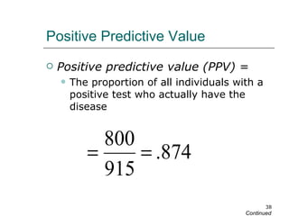
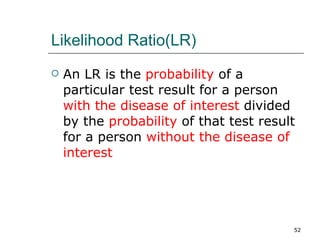
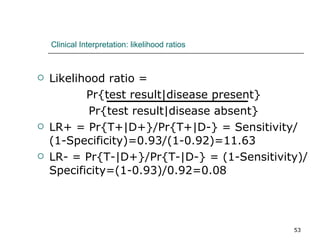
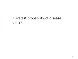
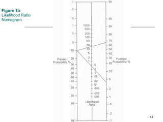
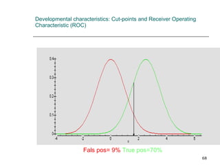
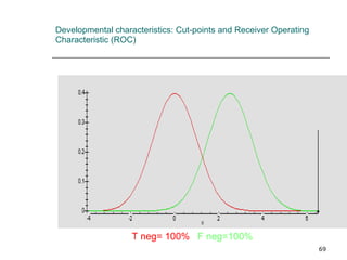
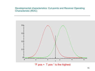
This document provides an overview of diagnostic testing and assessing diagnostic accuracy. It defines key concepts like sensitivity, specificity, predictive values, and likelihood ratios. Sensitivity measures the ability of a test to detect true positives, or people with the disease. Specificity measures the ability to detect true negatives, or people without the disease. Positive and negative predictive values depend on disease prevalence and estimate the probability of actual disease given a test result. Likelihood ratios quantify how much a test result changes the odds of disease. The document uses examples to demonstrate calculating and interpreting these performance measures.

1. Diagnostic Testing Prof. Wei-Qing Chen MD PhD Department of Biostatistics and Epidemiology School of Public Health 87332199 [email_address]

2. OBJECTIVES OF LECTURE understand that making a diagnosis is not black & white understand subclinical, preclinical disease understand accuracy (validity) of a diagnostic test understand the need for a ‘Gold Standard’ understand the indices by which accuracy is assessed understand reliability of a diagnostic test

3. Section A Diagnosis and Diagnostic Testing

4. Diagnosis Diagnosis is “the process determining health status and the factors responsible for producing it. Separating a target disease from health/other diseases Indicating that his outcome will be different (die earlier, suffer more, develop complications) Being indicative of treatment Changing the patterns following treatment

5. Way of diagnosis Collecting clinical data Symptoms: malaise, memory loss, fatigue, anxiety, etc. Signs: pale skin, hyperactive, red in face, etc. Special tests: cell count, x-ray, PB, cholesterolemia

6. Way of diagnosis Assembling a diagnostic entity (category) Diagnosis based on one variable: made by an “abnormal” value of a physiological function. Hypertension: SBP  160mmHg,or/and DBP  95mmHg, Anaemia: haemoglobin is less than 12mg% in adult women.

7. Way of diagnosis Assembling a diagnostic entity (category) Diagnosis based on several variable: made by an “abnormal” value of several physiological function. Metabolism syndrome: Hypertension, overweight, obesity in abdomen, high blood lipid, high blood glucose.

8. Diagnostic testing A “diagnostic test” originally is meant a test performed in a laboratory. In this chapter, including histories of disease, signs, symptoms, physical exams, special tests (x-ray, ECG, CT, cell counts, etc)

9. Section B Assessment on Diagnostic Testing

10. Diagnostic Tests Suppose a researcher had developed a new test for diagnosing the presence of disease A The new test is half the price of the current test for the same disease and can be administered during a routine checkup, as opposed to a half day hospital stay

11. Diagnostic Tests From a cost benefits perspective, this new test sounds like a winner However, before it becomes part of standard medical practice, it is important to evaluate the accuracy of this test compared to the existing technology

12. Is the diagnostic test valid??? Goal: Evaluate the “accuracy” of the new test

13. diagnose individuals for “disease” using both Gold standard (perfect) New diagnostic test The way to evaluate a new diagnostic test Continued

14. Selection of Gold standard A gold standard test is currently recognized as the most reliable test. Tissue diagnosis Radiological exam Autopsies Prolonged follow-up

15. Selection of subjects Target patients Patients diagnosed by “gold standard test” Typical and untypical patients Patients in early, middle and later period Light, middle and serious patients With and without complications

16. Selection of subjects Patients without target disease as control group Healthy persons are not suitable for as control group

17. Blindly comparing the results between the gold standard test and the new test

18. GOLD STANDARD (The Truth) Yes (+) No (–) Yes (+) No (–) Creating a 2 x 2 Table New Test True P False P False N True N

19. Dichotomous model Test true from Dichotomization Types of true True Positives = positive tests that are correct = a True Negatives = negative tests that are correct = d

20. Dichotomous model Test Errors from Dichotomization Types of errors False Positives = positive tests that are wrong = b False Negatives = negative tests that are wrong = c

21. DIAGNOSTIC ACCURACY OF A TEST Definition The extent to which the results of a diagnostic test reflect true disease status Terminology Accuracy / Validity interchangeable

22. Indicators for assessing diagnostic test

23. Measures of diagnostic accuracy Sensitivity Specificity Predictive values Measures of reliability / reproductivity Percent agreement

24. The ability of the test to detect the presence of disease (i.e. abnormality) The proportion of those with the disease who test positive (positive in disease, PID) True Positives True Positives + False Negatives a / a+c Sensitivity

25. Developmental characteristics: test parameters Sensitivity = Pr(T+|D+) = a/(a+c) Sensitivity is PID (Positive In Disease)

26. The ability of the test to detect freedom from disease (i.e. normality) The proportion of those without the disease who have a normal test (negative in health, NIH) True Negatives True Negatives + False Positives d / b+d Specificity

27. Developmental characteristics: test parameters Specificity = Pr(T-|D-) = d/(b+d) Specificity is NIH (Negative In Health)

28. Developmental characteristics: test parameters Pr(T+|D-) = F alse P ositive Rate ( FP rate) = b/(b+d)

29. Developmental characteristics: test parameters Pr(T-|D+) = F alse N egative Rate ( FN rate) = c/(a+c)

30. Developmental characteristics: test parameters Sensitivity = Pr(T+|D+) = 1 - FN rate Specificity = Pr(T-|D-) = 1 - FP rate

31. Example Accuracy of an exercise test for diagnosing coronary artery disease Screen: A random sample of 1,442 patients with symptoms of coronary artery disease Gold standard: Angiography New diagnostic test: Exercise tolerance test (ECG)

32. Resulting 2 x 2 Table Coronary Artery Disease (based on angiography) + – Exercise + 800 115 915 Tolerance test – 200 327 527 Test 1000 442 1442 Source: Weiner (1979) NEJM

33. Sensitivity and Specificity Sensitivity Proportion of those with disease who are positive on the new diagnostic test Continued

34. Sensitivity and Specificity Specificity Proportion of those without disease who are negative on the new diagnostic test

35. Positive and Negative Predictive Value Positive Predictive Value : Of all the people who tested positive for a disease, the proportion that actually has it Negative Predictive Value : Of all the people who tested negative for a disease, the proportion that actually does not have it In these patients, what you know are their test results, from which you are trying to determine whether they actually have the disease.

36. Positive Predictive Value Referring back to the exercise tolerance test: We want to know the chances of having coronary artery disease for someone who tests positive with the exercise tolerance test

37. Resulting 2 x 2 Table Coronary Artery Disease (based on angiography) + – Exercise + 800 115 915 Tolerance test – 200 327 527 Test 1000 442 1442 Source: Weiner (1979) NEJM

38. Positive Predictive Value Positive predictive value (PPV) = The proportion of all individuals with a positive test who actually have the disease Continued

39. Positive Predictive Value Positive predictive value (PPV) = “ Given that someone has a positive test result, what are the chances this person has the disease?” Continued

40. Positive Predictive Value This is not the same as sensitivity Sensitivity = “ Given that someone has the disease, what are the chances this person gets a positive result?”

41. Negative Predictive Value Referring back to the exercise tolerance test: We want to know the chances of not having coronary artery disease for someone who tests negative with the exercise tolerance test Continued

42. Negative Predictive Value Negative predictive value (NPV) = The proportion of all individuals with a negative test who do not have the disease

43. Negative Predictive Value Negative predictive value (NPV) = “ Given that someone has a negative test result, what are the chances this person does not have the disease?” Continued

44. Negative Predictive Value This is not the same as specificity Specificity = “ Given that someone does not have the disease, what are the chances this person gets a negative result?”

45. Notes on Interpretation The positive predictive value is 88% and the negative predictive value is 62% The sample was from a population of patients with symptoms of coronary artery disease Continued

46. Notes on Interpretation Interpretation If you have symptoms of coronary disease and you have a positive exercise test, there is an 88% chance you have coronary artery disease If you have a negative test result, there is a 62% you do not have coronary artery disease Continued

47. Notes on Interpretation However, in an asymptomatic population the positive predictive value might be much lower These estimates only apply to the population tested—the population of individuals with symptoms of coronary artery disease

48. Summary Sensitivity and specificity do not depend on prevalence of a disease and can always be estimated in a diagnostic test PPV and NPV do depend on the population prevalence of disease Continued

49. Summary If we start with a completely random sample, we can also estimate PPV and NPV for the population from which we have sampled If we want to estimate PPV and NPV for a different population we will need more machinery Continued

50. Summary If we over sample cases we will need more machinery to estimate PPV and NPV in a population with a given prevalence of disease

51. Likelihood Ratios and Post-Test Disease Probability

52. Likelihood Ratio(LR) An LR is the probability of a particular test result for a person with the disease of interest divided by the probability of that test result for a person without the disease of interest

53. Clinical Interpretation: likelihood ratios Likelihood ratio = Pr{test result|disease present} Pr{test result|disease absent} LR+ = Pr{T+|D+}/Pr{T+|D-} = Sensitivity/(1-Specificity)=0.93/(1-0.92)=11.63 LR- = Pr{T-|D+}/Pr{T-|D-} = (1-Sensitivity)/Specificity=(1-0.93)/0.92=0.08

54. Pretest probability of disease 0.13

55. Pretest odds of disease Pretest odds of disease are defined as the estimate before diagnostic testing of the probability that a patient has the disease of interest divided by the probability that the patient does not have the disease of interest. Pretest odds=Pretest probability/(1- Pretest probability) =0.13/(1-0.13=0.13/0.87=0.15

56. Posttest odds of disease Posttest odds of disease are defined as the estimate after diagnostic testing of the probability that a patient has the disease of interest divided by the probability that the patient does not have the disease of interest. Posttest odds=Pretest probability  LR + =0.15  11.63=1.76

57. Posttest probability Posttest probability=Posttest odds/(1+ Posttest odds) =1.76/(1+1.76)=1.76/2.76=0.64

58. Clinical interpretation of post-test probability Disease ruled out Disease ruled in

59. Advantages of LRs The higher or lower the LR, the higher or lower the post-test disease probability Which test will result in the highest post-test probability in a given patient? The test with the largest LR+ Which test will result in the lowest post-test probability in a given patient? The test with the smallest LR-

60. Advantages of LRs Clear separation of test characteristics from disease probability.

61. Likelihood Ratios - Advantage Provide a measure of a test’s ability to rule in or rule out disease independent of disease probability Test A LR+ > Test B LR+ Test A PV+ > Test B PV+ always! Test A LR- < Test B LR- Test A PV- > Test B PV- always!

62. Figure 1a : Likelihood Ratio Nomogram

63. Figure 1b : Likelihood Ratio Nomogram

64. Developmental characteristics: Cut-points and Receiver Operating Characteristic (ROC) Healthy

65. Developmental characteristics: Cut-points and Receiver Operating Characteristic (ROC) Healthy Sick

66. Developmental characteristics: Cut-points and Receiver Operating Characteristic (ROC) Fals pos= 20% True pos=82%

67. Developmental characteristics: Cut-points and Receiver Operating Characteristic (ROC) F pos= 100% T pos=100%

68. Developmental characteristics: Cut-points and Receiver Operating Characteristic (ROC) Fals pos= 9% True pos=70%

69. Developmental characteristics: Cut-points and Receiver Operating Characteristic (ROC) T neg= 100% F neg=100%

70. Developmental characteristics: Cut-points and Receiver Operating Characteristic (ROC) “ F pos + T pos “ is the highest

72. Developmental characteristics: Cut-points and Receiver Operating Characteristic (ROC) Receiver Operating Characteristic (ROC)

73. Developmental characteristics: Cut-points and Receiver Operating Characteristic (ROC) Receiver Operating Characteristic (ROC)

74. Receiver Operating Characteristic (ROC) ROC Curve allows comparison of different tests for the same condition without (before) specifying a cut-off point. The test with the largest AUC (Area under the curve) is the best.

76. Section C Diagnostic strategies

77. Combination tests: serial and parallel testing Combinations of specificity and sensitivity superior to the use of any single test may sometimes be achieved by strategic uses of multiple tests. There are two usual ways of doing this. Serial testing: Use >1 test in sequence, stopping at the first negative test. Diagnosis requires all tests to be positive. Parallel testing: Use >1 test simultaneously, diagnosing if any test is positive.

78. Combination tests: serial testing Doing the tests sequentially, instead of together with the same decision rule, is a cost saving measure. This strategy increases specificity above that of any of the individual tests, but degrades sensitivity below that of any of them singly. However, the sensitivity of the serial combination may still be higher than would be achievable if the cut-point of any single test were raised to achieve the same specificity as the serial combination.

79. Combination tests: serial testing Demonstration: Serial Testing with Independent Tests Se SC = sensitivity of serial combination Sp SC = specificity of serial combination Se SC = Product of all sensitivities= Se 1 X Se 2 X…etc Hence Se SC < all individual Se 1-Sp SC = Product of all(1-Sp) Hence Sp SC > all individual Sp i Serial test to rule-in disease

80. Combination tests: parallel testing Parallel Testing Usual decision strategy diagnoses if any test positive. This strategy increases sensitivity above that of any of the individual tests, but degrades specificity below that of any individual test. However, the specificity of the combination may be higher than would be achievable if the cut-point of any single test were lowered to achieve the same sensitivity as the parallel combination.

81. Combination tests: parallel testing Demonstration: Parallel Testing with Independent Tests Se PC = sensitivity of parallel combination Sp PC = specificity of parallel combination 1-Se PC = Product of all(1 - Se) Hence Se PC > all individual Se Sp PC = Product of all Sp Hence Sp PC < all individual Sp i Parallel test to rule-out disease

82. Clinical settings for parallel testing Parallel testing is used to rule-out serious but treatable conditions (example rule-out MI by CPK, CPK-MB, Troponin, and EKG. Any positive is considered positive) When a patient has non-specific symptoms, large list of possibilities (differential diagnosis). None of the possibilities has a high pretest probability. Negative test for each possibility is enough to rule it out. Any positive test is considered positive.

83. Because specificity is low, further testing is now required (serial testing) to make a diagnosis (Sp P In).

84. Clinical settings for serial testing When treatment is hazardous (surgery, chemotherapy) we use serial testing to raise specificity.(Blood test followed by more tests, followed by imaging, followed by biopsy).

85. Calculate sensitivity and specificity of parallel tests (Serial tests in HIV CDC exercise) 2 tests in parallel 1 st test sens = spec = 80% 2 nd test sens = spec = 90% 1-Sensitivity of combination = (1-0.8)X(1-0.9)=0.2X0.1=0.02 Sensitivity= 98% Specificity is 0.8 X 0.9 = 0.72

86. Increasing the prevalence of disease Referral process Selected demographic groups Specific of the clinical situation

87. Effect of prevalence on predictive value(Se=70%, Sp=90%) 93.0 50,000 Clinical suspicious prostatic nodule 5.6 500 Men, age 75or greater 0.4 35 General population PPV (%) Prevalence (case/100,000) Setting

88. Lead Time 1990 1997 2000 death Diagnosis and treatment Biologic onset of disease 1990 1994 2000 death Biologic onset of disease Screening: diagnosis & treatment

89. Length Bias 1995 2000 death Biologic onset of disease 1989 1994 death Biologic onset of disease Screening: diagnosis & treatment 2002 1994 Screening:

90. Thanks!!!