MFR, b value

1. Bulletin of the Seismological Society of America, Vol. 72, No. 5, pp. 1677-1687, October 1982
THE STANDARD ERROR OF THE MAGNITUDE-FREQUENCY b VALUE
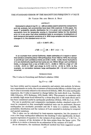
BY YAOLIN SHI AND BRUCE A. BOLT
ABSTRACT
Estimated b values in log N = a - bM are widely used in seismicity comparisons
and risk analysis, but uncertainties have been little explored. In this paper, the
usual F probability density distribution for b is given and compared with an
asymptotic form for temporally varying b. Convenient tables for the standard
error of b are given that allow statistical tests to accompany investigations of
both temporal and spatial variations of b. With large samples and slow temporal
changes in b, the standard error of b is
where
o(l~) = 2.30b2a (?~) ,
n
a2(M ) = T (M,- K.f)2 /n(n- 1).
i=1
In an example from central California, stable estimates of b require a space-
time window containing about 100 earthquakes. From 1952 to 1978, the average
b and 90 per cent confidence limits are 0.95 (+0.94, -0.30). Some fluctuations
of b are statistically significant but some are not. Within 90 per cent confidence
limits, b changes from a low of 0.60 (+0.11, -0.09) in 1955 to a high of 1.39
(+0.25, -0.21) in 1967 and drops to 0.72 (+0.13, -0.10) in 1975. In this
example, no correlation between large earthquakes (M > 5) and b variations
occurred.
INTRODUCTION
The b value in Gutenberg and Richter's relation (1954)
log N = a- bM (1)
has been widely used in research on seismicity and seismic risk analysis. In labora-
tory experiments on rocks, the occurrence of microcracks follows a similar form, and
the b value is inversely related to the stress level (Scholz, 1968). For some earthquake
sequences, the b value is reported to change before the main shock (e.g., Suyehiro,
1966; Gibowicz, 1973; Robinson, 1979; Smith, 1981). This property is consistent with
an initially high stress level followed by a stress drop due to the main shock and it
has been considered useful in earthquake prediction (Scholz, 1968; Li et al., 1978).
For use in prediction and comparative mechanism studies, standard errors of b
must be computed so that meaningful statistical tests can be performed. Because
earthquakes are stochastic processes and the b value is a random variable, the
probability distribution and the variance of b are essential in studying its temporal
and spatial variations.
The b value can be calculated by least-squares regression, but the presence of
even a few large earthquakes influences the resulting b value significantly. In least-
squares regression of equation (1), the variance of one observation, a 2 = Eri2/(n - 1),
is only a measure of the deviation of the data points from the linear curve. The
problem is to derive a formula for an estimation of the variance of b itself.
As an alternative, the maximum likelihood method has been suggested as pref-
1677

2. 1678 YAOLIN SHI AND BRUCE A. BOLT
erable for calculating the b value because it yields a more robust estimate when the
number of the infrequent large earthquakes changes. There will be cases, however,
such as estimating the probability of the largest magnitude of earthquakes from
relation (1), where the least-squares method is more suitable.
Suppose the probability density of magnitude M is exponential with mean 1/fi,
i.e.,
fi exp{-fi(M - M0)}, M > Mo. (2)
The maximum likelihood estimation of fi(b = fi log e) is (Aki, 1965; Utsu, 1965)
1
(3)P = -M - Mo'
where 2~ris the mean magnitude and Mo is the smallest (or "threshold") magnitude
considered. In these seminal papers, only an approximate formula to estimate the
variance of b was given.
First, confidence limits need to be defined. If we form a linear combination Y so
that
n
Y= E Y~, (4)
i=l
where, in terms of the density function, yi = O/Off log f(Mi, fi), it can then be shown
(e.g., Aki, 1965) that for large n, Y has a normal distribution with a zero mean and
variance n / fi 2.
The probability that
-dE < --=fly < dE (5)
is given by
- - exp(-x2/2) dx. (6)
• = ~ d~
Then e = 95 per cent if d~ = 1.96 and • = 90 per cent if dE = 1.65. When defined in
this way, the confidence level is directly related only to Y, and consequently, it is
difficult to assess information about the distribution of b itself.
More directly, the distribution of/~ is
[~ =~2nfi/X~,~ = ~F~,2n. (7)
This chi-squared form is given by Utsu (1966) and rederived by Zhang and Song
(1981). In brief,
n
M - Mo =-I ~ (Mi- Mo)
ni=l
1 n
=- 2 e,/fi,
ni=l

3. THE STANDARD ERROR OF THE MAGNITUDE-FREQUENCY b VALUE 1679
where ei are independent unit exponentials that are distributed like X22/2. Then,
from the additivity property of X2,
- Mo d X~n/2nfi.
It follows from (7) (see Abramowitz and Stegun, 1965, 26.6.3) that
E(fi)=fin/(n-1), n>l (8)
var fi = fi2n2/[(n - 1)2(n - 2)], n > 2. (9)
Zhang and Song (1981) concluded from (8) that the maximum likelihood method
yields a biased estimation of b, and they also investigated, by a Monte Carlo
procedure, the least-squares estimate of the standard error of b. The formula fl/~n
(Aki, 1965) is an approximation to (9).
Once the distribution is derived, confidence intervals can be found by using tables
of F or X2 distributions, e.g., for 0.90 per cent confidence level
F~,2n(0.05) < ~ < F~,2n(0.95) (10)
or
2nb
X22n(0.05) < A < X22n(0.95). (11)
b
Appropriate tables are not readily available in the seismological literature for
n > 50, but graphs giving the cumulative distribution of the ratio (10) are given by
Utsu (1966).
In the above work, b was considered a constant in time. We will discuss the
distribution of b and estimate its standard error for both constant and slowly
changing b. Our results are then checked by comparison with real earthquake
sequences.
NUMERICAL FORMULA
We will now take an alternative approach to the distribution of b and consider
the distribution of Mi without any assumption of the constancy of b. By the central
n
limit theorem, the distribution function of M, M = _1 ~ Mi, approaches a normal
ni=l
distribution for large n if each Mi has finite mean and variance, and the M~ are
independent. Therefore, in the limit, the distribution of 3~t can be expressed as
1
f(3I) - exp(-(Al - E(2~r))2/2 var 214).
~/2~ var 214
From (2),
1
E (M) = 214o+ -
B
1
var M -
B ~
1
E(3YI) = E(M) = Mo + -
1
var AI = - var M = 1~nil 2.
n
(12)

4. 1680 YAOLIN SHI AND BRUCE A. BOLT
Because fi (3)) is a monotonically decreasing function of 3I, there exists a single-
valued inverse fimction
~(j~) = i
-~ + Mo. (13)
P
Then the distribution of b is
-- ^
1 log e
= ~/2~ var3) ~2 exp(-(1/b- 1//~)2log2e/2 var3))
where/~ = log e/[E (3)) - M0]. Typical results are shown in Figure 1.
3 0
(14)
2
<_Q
1
0 4.04.55.0
,i
.51.01.52.02.53.03.5
b value
FIG. 1. Density functionsg(b) calculated from (14) and (15a). Light line for b = 1.6, o_~ = 0.1; heavy
line for b = 1.6, n = 20 (or o114 = 0.05); dashed line for b = 1.0, n = 30.
Here the distribution function of/~, is given for large n; the mean and variance of
3), and then of/~, can be calculated from earthquake catalogs. Statistical tests can,
as a consequence, be carried out conveniently by table reference. Because the value
of b in a region is observed to change with time and location, its mean and variance
might also be expected to change. In other words, b should be regarded, in general,
as a nonstationary stochastic process b (t). When sampling with a small time and
space window, however, b can be usually taken as stationary and with constant
expectation. Then, the above formulas hold and the distribution function g(/~ ) can
be expressed simply as
g(/~) = ~-~ b
exp(-n(b/[~ - 1)2/2). (15a)

5. THE STANDARD ERROR OF THE MAGNITUDE-FREQUENCY b VALUE 1681
For comparison, the exact formula for g(/~ ) for constant b is (Utsu, 1966)
express the sampling weight at different times. Then
g(/~) - n ~ b ~
(n- 1)! /~#Ji exp(-nb/b). (15b)
Sample confidence levels, calculated from (15) are given in Table 1 and may be
TABLE 1
PERCENTAGE POINTS FOR THE DISTRIBUTION OF g(b) AND n
ConfidenceLevel 0.90
bin
30 50 100 200
0.4 -0.10 -0.08 -0.06 -0.04
0.14 0.11 0.07 0.05
0.5 -0.13 -0.10 -0.07 -0.05
0.18 0.13 0.09 0.06
0.6 -0.15 -0.12 -0.09 -0.06
0.21 0.16 0.11 0.07
0.7 -0.18 -0.14 -0.10 -0.08
0.25 0.19 0.13 0.09
0.8 -0.20 -0.16 -0.12 -0.09
0.29 0.21 0.14 0.10
0.9 -0.23 -0.18 -0.13 -0.10
0.32 0.24 0.16 0.11
1.0 -0.25 -0.20 -0.15 -0.11
0.36 0.27 0.18 0.12
1.1 -0.28 -0.22 -0.16 -0.12
0.39 0.29 0.20 0.14
1.2 --0.30 -0.24 --0.18 --0.13
0.43 0.32 0.22 0.15
1.3 -0.33 -0.26 -0.19 -0.14
0.46 0.35 0.24 0.16
1.4 -0.35 -0.28 -0.21 -0.15
0.50 0.37 0.25 0.17
1.5 -0.38 -0.30 -0.22 -0.16
0.54 0.40 0.27 0.19
1.6 -0.40 -0.32 -0.24 -0.17
0.57 0.43 0.29 0.20
1.7 -0.43 --0.35 -0.25 -0.18
0.61 0.45 0.31 0.21
1.8 -0.45 -0.37 -0.27 -0.19
0.64 0.47 0.33 0.22
1.9 -0.48 -0.39 -0.28 -0.21
0.68 0.51 0.34 0.24
2.0 -0.50 -0.41 -0.30 -0.22
0.71 0.53 0.36 0.25
checked against standard X~ tables. Differences between (15a) and (15b) are not
large for large n.
Formula (15b) is important not only because of the assumption that a constant b
within a small sampling window may be acceptable in many cases, but also because
most published b values are given without standard errors and var 2tl. This omission
means that they cannot be used with formula (14) nor for quantitative statistical
tests. Formula (15b) allows, however, the upper limits of the standard error of b

6. 1682 YAOLIN SHI AND BRUCE A. BOLT
values to be estimated, as illustrated later. In this way, b values can be used for
statistical tests.
When b changes with time, a distribution function of b, f(b, t), can be assigned
and
t-
vat b = I (b - E(b))2f(b, t) db dt. (16)
2
If b changes slowly with time, f(b, t) can be decomposed to
f(b, t) = g(b)w(t), (17)
where g(b) is defined earlier. At any time, b has the same form of distribution
function as (14), although its mean and variance may change. Let function w(t)
express the sampling weight at different times. Then
var b = f (b- E(b)}2g(b)w(t) db dt
C
= J ((b -/~t) + (E - E(b))}2g(b)w(t) db dt
= (var bt ) "t- var/~,
where bt is the expectation of b at time t, i.e.,
-- I bg(b)5t db
J
(18)
(19)
and ( ) indicates the time average. Thus, because the cross-product terms vanish,
the variance of b is composed of two parts. The first part is the time average of the
variance of b at different times as calculated previously. The second part is the
variance of 6, the mean of b averaged over the whole time range.
Because var b = (var be), formula (15b) may give an underestimated standard
error when the temporal and spatial window is too large for b to be constant. In this
case, we have to estimate the average 214and var M = ~ (Mi - M)2/n(n - 1), and
j=l
then determine the probability interval of b from Table 2, computed using (14).
In the general case, a large sample distribution of/~ can be derived in the usual
way. Let Xi = Mi - Mo. Then/~ = 1~. IfXi has mean/t and variance a 2, it can be
shown as a special case of (14) that fi is asymptotically normal with mean 1//z and
variance
(llt~e)2a21n = fl4o21n. (20)
n
Here o2 may be estimated, as above, from ~ (Mi - -ff/I)2/(n - 1). Note that log/~
i=l
is also asymptotically normal with mean log fi and variance fl2o2/n. These functions
may also fluctuate with time. It also follows that for large n,
b~
o(/~)= ~ o(M) = 2.3052~(M). (21)
In practice, starting from an earthquake catalog, we can estimate b by maximum
likelihood from M using (3). We can also obtain a probability interval for b from

7. THE STANDARD ERROR OF THE MAGNITUDE-FREQUENCY b VALUE 1683
formula (15), (Table 1) or formula (14), (Table 2) depending on whether the b value
can be regarded as an approximate constant or not. Brillinger (personal communi-
cation) describes the model contemplated as "doubly stochastic." The process
b (M, t) may, of course, depend not only on t, but also on M, and it is an assumption
that the distribution of/~ remains exponential in these cases.
TABLE 2
PERCENTAGE POINTS FOR THE DISTRIBUTION OF g(b) AND
ConfidenceLevel0.90
b/(J)71
0.15 0.10 0.05 0.03
0.4 -0.07 -0.05 -0.03 -0.01
0.12 0.07 0.04 0.02
0.5 -0.11 -0.08 -0.04 -0.02
0.20 0.12 0.05 0.03
0.6 -0.15 -0.11 -0.06 -0.04
0.31 0.18 0.08 0.05
0.7 -0.20 -0.14 -0.08 -0.05
0.46 0.26 0.11 0.06
0.8 -0.25 -0.18 -0.10 -0.06
0.67 0.35 0.15 0.08
0.9 -0.30 -0.23 -0.13 -0.08
0.94 0.47 0.19 0.11
1.0 -0.36 -0.27 -0.16 -0.10
1.32 0.61 0.24 0.13
1.1 -0.42 -0.32 -0.19 -0.12
1.84 0.79 0.29 0.16
1.2 -0.50 -0.38 -0.22 -0.14
3.20 0.99 0.36 0.19
1.3 -0.55 -0.43 -0.25 -0.16
3.67 1.26 0.43 0.23
1.4 -0.62 -0.48 -0.29 -0.19
5.44 1.58 0.51 0.27
1.5 -0.69 -0.54 -0.33 -0.22
8.64 1.98 0.60 0.31
1.6 -0.76 -0.60 -0.37 -0.24
15.97 2.46 0.70 0.36
1.7 -0.84 -0.66 -0.41 -0.27
47.97 3.08 0.81 0.41
1.8 -0.91 -0.73 -0.46 -0.30
--* 3.86 0.93 0.47
1.9 -0.99 -0.79 -0.50 -0.32
-- 4.88 1.07 0.53
2.0 -1.07 -0.86 -0.55 -0.37
-- 6.26 1.22 0.59
* -- > 100.
CENTRAL CALIFORNIASEISMICITY
The seismicity in central California is taken as an example. The catalog is
considered complete for earthquakes with M _->2.5 in this region since 1952 (Bolt
and Miller, 1975). The sample has 2572 earthquakes in 22 yr.
Through a time window containing n = 30, 50, 100, and 200 earthquakes,
respectively, b values were scanned in the time domain. Two distinct b (t) curves for
n = 30 and n = 200 are plotted in Figures 2 and 3. Error bars for the 90 per cent

8. 1684 YAOLIN SI-II AND BRUCE A. BOLT
~7~--~ ur~ (M
r~
r~
o~
r~
r~
r~
cD
CO
r~
~o
~o
~o
o
~o
oo
CD
~o
kn
t--
un
c~
kn
U3
u~
u~
t~
c,-J
anloA q
h~
A~
8~
c~

9. THE STANDARD ERROR OF THE MAGNITUDE-FREQUENCY b VALUE
co
1685
OJ(M
~Ldu u
~d
o
u
~d~d
Lr~ C) I~ 0 LF]
F~
Ld
m~
o
r~
o~
~o
co
r~
Lo
tD
Lrl
CO
m-
tO
CO
~J
~0
~0
C3
~0
Cn
~q
CO
bq
I
m
LA
(.0
Ln
LN
cDLn
LJ
t--
II
8
!
c6
anlDA q

10. 1686 YAOLIN SHI AND BRUCE A. BOLT
confidence level are evaluated from Table 1 (formula 15). For comparison, error
intervals were also evaluated from Table 2 (formula 14). These comparisons show
that although for small time windows (e.g., n = 30), the estimates sometimes differ
by over 100 per cent, for larger time windows (e.g., n = 100), the error intervals
calculated from the two formulas are almost the same. This implies that the variance
of b can be estimated from previous published data of b, even if var M is not given,
provided n is not too small.
For a time window containing n = 30 earthquakes, the b(t) curve has more
fluctuations than for the case n = 200. However, many such fluctuations are not
statistically significant when the chance variation is considered, and this result must
be taken into account if changes of b value are used as a precursor in earthquake
prediction [c.f. Wyss and Lee {1973)].
Over a longer time interval, significant temporal variations of b are obvious in
Figure 3. (Alternatively, log /~ could be graphed in Figures 2 and 3 so that the
3.0
V
2.5
2.0
1.5
1.0
f -- i i i i
• 5 .0 ] .5 2.0 2.5 3.0 ~.5 4.0 4.5 5.0
b vo lue
FIG. 4. Histogram of b distribution for central C~lifornia seismicity, from 397 windows each containing
100 earthquakes, compared with theoretical curve b = 0.95, aM = 0.13.
confidence intervals have constant width. The hypotheses of time invariant b may
then be tested by calculating the proportion of b values that exceed the intervals.)
The times of occurrence of earthquakes larger than magnitude 5 are also plotted in
the figure. The value of b changes from a low level of 0.60 (+0.11, -0.09) in 1955 to
a high value of 1.39 (+0.25, -0.21) in 1967 and drops again to 0.72 (+0.13, -0.10) in
1975. However, we can find no correlation between changes of b and the time of
occurrence of the larger earthquakes. The meaning of this longer term variation of
b is not yet clear.
Finally, the histogram of observed b since 1952 is plotted in Figure 4. The
theoretical distribution curve of/~ = 0.95 and oM = 0.13 is also drawn. Because
within the 22-yr period b changed with time, formula (15) cannot be used. The
theoretical curve is calculated from (14) and a X2 test made with the histogram
grouped into 10 intervals. The computed X~o= 17.5 is close to the expected value of
18.3 for 10 degrees of freedom at the 5 per cent significance level. Therefore, the

11. THE STANDARD ERROR OF THE MAGNITUDE-FREQUENCY b VALUE 1687
evidence does not suggest that the actual distribution differs from the derived
theoretical form at this level.
It should be emphasized that the uncritical use of formula (15) leads to a 90 per
cent confidence level estimate for b of 0.95 (+0.17, -0.14) and a standard error of
0.10. In a similar way, the simple application of the formula of Aki (1965) or Zhang
and Song (1981) yields 0.95 (±0.10) for the standard error. Slow changes of b with
time entail a broader b distribution. From equation (21), the large sample approxi-
mation gives 0.95 (__0.27) for the standard error for the observed distribution of
slowly varying b in central California. We calculate also that the 90 per cent
confidence level of b is more realistically 0.95 (+0.94, -0.30). The result implies that
even large differences between long-term average b values for different regions or
epochs or focal depths (Gutenberg and Richter, 1954) may not be significant.
ACKNOWLEDGMENTS
The authors thank Professor D. Brillinger, Dr. R. Uhrhammer and a reviewer, and A. Lees for helpful
discussions and suggestions. The computer time was provided by the Computer Center of the University
of California, Berkeley.
REFERENCES
Abramowitz, M. and I. A. Stegun (1965). Handbook of Mathematical Functions, U.S. Department of
Commerce, National Bureau of Standards.
Aki, K. (1965). Maximum likelihood estimate of b in the formula log N = a - bM and its confidence
limits, Bull. Earthquake Res. Inst., Tokyo Univ. 43, 237-239.
Bolt, B. A. and R. D. Miller (1975). Catalog of earthquakes in northern California and adjoining areas,
Seismographic Stations, University of California, Berkeley.
Gibowicz, S. J. (1973). Variation of the frequency-magnitude relation during earthquake sequences in
New Zealand, Bull. Seism. Soc. Am. 63, 517-528.
Gutenberg, B. and C. F. Richter (1954). Seismicity of the Earth, 2nd ed., Princeton University, Princeton,
New Jersey.
Li, Q.-L., J.-B. Chen, L. Yu, and B.-L. Hao (1978}. Time and space scanning of the b value--A method
for monitoring the development of catastrophic earthquakes, Acta Geophys. Sin. 21, 101-125.
Robinson, R. (1979). Variation of energy release, rate of occurrence and b value of earthquakes in the
main seismic region, New Zealand, Phys. Earth Planet. Interiors 18, 209-220.
Scholz, C. (1968). The frequency-magnitude relation of microfracturing in rock and its relation to
earthquakes, Bull. Seism. Soc. Am. 58, 399-415.
Smith, W. D. (1981). The b-value as an earthquake precursor, Nature 289, 136-139.
Suyehiro, S. (1966). Differences between aftershocks and foreshocks in the relationship of magnitude to
frequency of occurrence for the great Chilean earthquake of 1960, Bull. Seism. Soc. Am. 56, 185-200.
Utsu, T. (1965). A method for determining the value of b in formula log N = a - bM showing the
magnitude-frequency relation for earthquakes, Geophys. Bull. Hokkaido Univ. 13, 99-103.
Utsu, T. (1966). A statistical significance test of the difference in b-value between two earthquake groups,
J. Phys. Earth 14, 37-40.
Zhang, J.-Z. and L,-Y. Song (1981). On the method of estimating b value and its standard error, Acta
Seismologica Sin. 3, 292-301.
Wyss, M. and W. H. K. Lee {1973). Proc. conf. on tectonic problems on the San Andreas fault system 13,
24-42, Stanford University, Stanford, California.
SEISMOGRAPHICSTATIONS
DEPARTMENT OF GEOLOGYAND GEOPHYSICS
UNIVERSITY OF CALIFORNIA
BERKELEY, CALIFORNIA 94720
Manuscript received 15 March 1982