Completeness

1. 684
Bulletin of the Seismological Society of America, Vol. 95, No. 2, pp. 684–698, April 2005, doi: 10.1785/0120040007
Assessing the Quality of Earthquake Catalogues: Estimating the Magnitude
of Completeness and Its Uncertainty
by Jochen Woessner and Stefan Wiemer
Abstract We introduce a new method to determine the magnitude of complete-
ness Mc and its uncertainty. Our method models the entire magnitude range (EMR
method) consisting of the self-similar complete part of the frequency-magnitude dis-
tribution and the incomplete portion, thus providing a comprehensive seismicity
model. We compare the EMR method with three existing techniques, finding that
EMR shows a superior performance when applied to synthetic test cases or real data
from regional and global earthquake catalogues. This method, however, is also the
most computationally intensive. Accurate knowledge of Mc is essential for many
seismicity-based studies, and particularly for mapping out seismicity parameters such
as the b-value of the Gutenberg-Richter relationship. By explicitly computing the
uncertainties in Mc using a bootstrap approach, we show that uncertainties in b-values
are larger than traditionally assumed, especially when considering small sample sizes.
As examples, we investigated temporal variations of Mc for the 1992 Landers
aftershock sequence and found that it was underestimated on average by 0.2 with
former techniques. Mapping Mc on a global scale, Mc reveals considerable spatial
variations for the Harvard Centroid Moment Tensor (CMT) (5.3 Յ Mc Յ 6.0) and
the International Seismological Centre (ISC) catalogue (4.3 Յ Mc Յ 5.0).
Introduction
Earthquake catalogues are one of the most important
products of seismology. They provide a comprehensive data-
base useful for numerous studies related to seismotectonics,
seismicity, earthquake physics, and hazard analysis. A criti-
cal issue to be addressed before any scientific analysis is to
assess the quality, consistency, and homogeneity of the data.
Any earthquake catalogue is the result of signals recorded
on a complex, spatially and temporally heterogeneous net-
work of seismometers, and processed by humans using a
variety of software and assumptions. Consequently, the re-
sulting seismicity record is far from being calibrated, in the
sense of a laboratory physical experiment. Thus, even the
best earthquake catalogues are heterogeneous and inconsis-
tent in space and time because of networks’ limitations to
detect signals, and are likely to show as many man-made
changes in reporting as natural ones (Habermann, 1987; Ha-
bermann, 1991; Habermann and Creamer, 1994; Zuniga and
Wiemer, 1999). Unraveling and understanding this complex
fabric is a challenging yet essential task.
In this study, we address one specific aspect of quality
control: the assessment of the magnitude of completeness,
Mc, which is defined as the lowest magnitude at which 100%
of the events in a space–time volume are detected (Rydelek
and Sacks, 1989; Taylor et al., 1990; Wiemer and Wyss,
2000). This definition is not strict in a mathematical sense,
and is connected to the assumption of a power-law behavior
of the larger magnitudes. Below Mc, a fraction of events is
missed by the network (1) because they are too small to be
recorded on enough stations; (2) because network operators
decided that events below a certain threshold are not of in-
terest; or, (3) in case of an aftershock sequence, because they
are too small to be detected within the coda of larger events.
We compare methods to estimate Mc based on the as-
sumption that, for a given volume, a simple power-law can
approximate the frequency-magnitude distribution (FMD).
The FMD describes the relationship between the frequency
of occurrence and the magnitude of earthquakes (Ishimoto
and Iida, 1939; Gutenberg and Richter, 1944):
log N(M) ‫ס‬ a ‫מ‬ bM, (1)10
where N(M) refers to the frequency of earthquakes with
magnitudes larger or equal than M. The b-value describes
the relative size distribution of events. To estimate the b-
value, a maximum-likelihood technique is the most appro-
priate measure:
log (e)10
b ‫ס‬ . (2)
DMbin͗M͘ ‫מ‬ M ‫מ‬c΄ ΂ ΋ ΃΅2

2. Assessing the Quality of Earthquake Catalogues: Estimating the Magnitude of Completeness and Its Uncertainty 685
Here ͗M͘ is the mean magnitude of the sample and DMbin is
the binning width of the catalogue (Aki, 1965; Bender, 1983;
Utsu, 1999).
Rydelek and Sacks (2003) criticized Wiemer and Wyss
(2000), who had performed detailed mapping of Mc, for us-
ing the assumption of earthquake self-similarity in their
methods. However, Wiemer and Wyss (2003) maintain that
the assumption of self-similarity is in most cases well
founded, and that breaks in earthquake scaling claimed by
Rydelek and Sacks (2003) are indeed caused by temporal
and spatial heterogeneity in Mc. The assumption that seismic
events are self-similar for the entire range of observable
events is supported by studies of, for example, von Seggern
et al. (2003) and Ide and Beroza (2001).
A “safe” way to deal with the dependence of b- and a-
values on Mc is to choose a large value of Mc, but this seems
overly conservative. However, this approach decreases the
amount of available data, reducing spatial and temporal res-
olution and increasing uncertainties due to smaller sample
sizes. Maximizing data availability while avoiding bias due
to underestimated Mc is desirable; moreover, it is essential
when one is interested in questions such as studying breaks
in magnitude scaling (Abercrombie and Brune, 1994; Kno-
poff, 2000; Taylor et al., 1990; von Seggern et al., 2003).
Unless the space–time history of Mc ‫ס‬ Mc(x,y,z,t) is taken
into consideration, a study would have to conservatively as-
sume the highest Mc observed. It is further complicated by
the need to determine Mc automatically, since in most ap-
plications, numerous determinations of Mc are needed when
mapping parameters such as seismicity rates or b-values
(Wiemer and Wyss, 2000; Wiemer, 2001).
A reliable Mc determination is vital for numerous seis-
micity- and hazard-related studies. Transients in seismicity
rates, for example, have increasingly been scrutinized, as
they are closely linked to changes in stress or strain, such as
static and dynamic triggering phenomena (e.g., Gomberg
et al., 2001; Stein, 1999). Other examples of studies that are
sensitive to Mc are scaling-related investigations (Knopoff,
2000; Main, 2000) or aftershock sequences (Enescu and Ito,
2002; Woessner et al., 2004). In our own work on seismic
quiescence (Wiemer and Wyss, 1994; Wyss and Wiemer,
2000), b-value mapping (Wiemer and Wyss, 2002; Gersten-
berger et al., 2001), and time-dependent hazard (Wiemer,
2000), for example, we often found Mc to be the most critical
parameter of the analysis. Knowledge of Mc(x,y,z,t) is im-
portant, because a minute change in Mc in DMc ‫ס‬ 0.1 leads
(assuming b ‫ס‬ 1.0) to a 25% change in seismicity rates; a
change of DMc ‫ס‬ 0.3 reduces the rate by a factor of two.
The requirements for an algorithm to determine Mc in
our assessment are: (1) to calculate Mc automatically for a
variety of datasets; (2) to give reliable uncertainty estimates;
and (3) to conserve computer time. We specifically limit our
study to techniques based on parametric data of modern
earthquake catalogues. A number of researchers have inves-
tigated detection capability by studying signal-to-noise ra-
tios at particular stations (Gomberg, 1991; Kvaerna et al.,
2002a,b); however, these waveform-based techniques are
generally too time-consuming to be practical for most stud-
ies. We also focus on recent instrumental catalogues, ignor-
ing the question of how to best determine Mc in historical
datasets commonly used in seismic hazard assessment (Al-
barello et al., 2001; Faeh et al., 2003). In order to evaluate
the performance of the different algorithms, we use syn-
thetically-created regional and global data sets.
We believe that the review and comparison of adaptable
methods presented in this article, and the introduction of
uncertainties in Mc, are an important contribution for im-
proving seismicity related studies.
Data
For the comparison of methods to determine Mc, we
chose subsets of six different catalogues with diverse prop-
erties. The catalogues analyzed are freely available from the
websites of the specific agencies:
• Regional catalogue: We selected a subset of the Earth-
quake Catalogue of Switzerland (ECOS) of the Swiss Seis-
mological Service (SSS) in the southern province Wallis
for the period 1992–2002 (Fig. 1A), providing a local
magnitude ML (Deichmann et al., 2002).
• Regional catalogue: We chose a subset of the Northern
California Seismic Network (NCSN) catalogue focused on
the San Francisco Bay area for the period 1998–2002, us-
ing the preferred magnitude (Fig. 1B).
• Volcanic region: We use a subset of the earthquake cata-
logue maintained by the National Research Institute for
Earth Science and Disaster Prevention (NIED) reporting a
local magnitude ML. The subset spans a small volcanic
region in the Kanto province for the period 1992–2002
(Fig. 1C).
• Aftershock sequence: We selected a seven year period
(1992–1999) from the Landers 1992 MW 7.3 aftershock
sequence, using the earthquakes recorded by the Southern
California Seismic Network (SCSN), a cooperative project
of Caltech and the U.S. Geological Survey, distributed
through the Southern California Earthquake Data Center
(SCEDC), reporting a local magnitude ML (Fig. 1D).
• Global datasets:
a. the Harvard Centroid Moment Tensor (CMT) cata-
logue, reporting the moment magnitude MW, is used
for the time period 1983–2002. Only shallow events
(d Յ 70km) are used for mapping purposes.
b. the International Seismological Centre (ISC) catalogue
is analyzed for the period 1980–2000 and magnitudes
mb Ն 4.3. Only shallow events (d Յ 70km) are used.
The cut-off magnitude was chosen due to the temporal
heterogeneity of the catalogue. Surface wave magni-
tudes are taken to equal mb in case there is none.
From this point on, we refer to the generic expression

3. 686 J. Woessner and S. Wiemer
Figure 1. Earthquakes used in this study: (A) Subset of the earthquake catalogue
of Switzerland (ECOS) in the southern province Wallis; (B) subset of the NCSN cata-
logue comprising the San Francisco Bay area; (C) subset of the NIED catalogue in the
Kanto province with the triangles indicating volcanoes; and (D) the Landers 1992
aftershock sequence from the SCSN catalogue. California maps display known faults
in light gray.
“magnitude” that corresponds to the magnitude of the re-
spective earthquake catalogue outlined above.
Methods
Methods to estimate the magnitude of completeness of
earthquake catalogues are based on two fundamentally dif-
ferent assumptions. Most methods assume self-similarity of
the earthquake process, which consequently implies a
power-law distribution of earthquakes in the magnitude and
in the seismic moment domain. One other approach relies
on the assumption that the detection threshold due to noise
decreases at night, thus the magnitude of completeness is
determined using the day-to-night ratio of earthquake fre-
quency (Rydelek and Sacks, 1989; Taylor et al., 1990).
In this study, we compare only methods assuming self-
similarity of the earthquake process:
1. Entire-magnitude-range method (EMR) modified from
Ogata and Katsura (1993)
2. Maximum curvature-method (MAXC) (Wiemer and
Wyss, 2000)
3. Goodness-of-fit test (GFT) (Wiemer and Wyss, 2000)
4. Mc by b-value stability (MBS) (Cao and Gao, 2002)
These methods are described below and are illustrated
schematically in Figure 2. The code is freely available to-
gether with the seismicity analysis software package ZMAP
(Wiemer, 2001), which is written in Mathworks’ commercial
software language Matlab௡ (http://www.mathworks.com).

4. Assessing the Quality of Earthquake Catalogues: Estimating the Magnitude of Completeness and Its Uncertainty 687
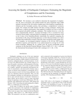
Figure 2. EMR method applied to the NCSN-catalogue
data (1998–2001): Mc ‫ס‬ 1.2, b ‫ס‬ 0.98, a ‫ס‬ 5.25, l ‫ס‬
0.73, r ‫ס‬ 21. (A) Cumulative and non-cumulative FMD and
model on logarithmic scale with the arrow indicating Mc.
(B) Normal CDF fit (gray line) to the data below Mc ‫ס‬ 1.2
on linear scale. Standard deviations of the model, dashed
gray line; original data, diamonds; non-cumulative FMD of
EMR-model, circles. (C) Choice of the best model from the
maximum-likelihood estimates denoted with an arrow point-
ing to the resulting Mc-value.
EMR Method
We developed a method to estimate Mc that uses the
entire data set, including the range of magnitudes reported
incompletely. Our approach is similar to that of Ogata and
Katsura (1993), and uses a maximum-likelihood estimator
for a model that consists of two parts: one to model the
complete part, and one to sample the incomplete part of the
frequency-magnitude distribution (Fig. 2). We use the entire
magnitude range to obtain a more robust estimate of Mc,
especially for mapping purposes.
For data above an assumed Mc, we presume a power-
law behavior. We compute a- and b-values using a maximum-
likelihood estimate for the a- and b-value (Aki, 1965; Utsu,
1965). For data below the assumed Mc, a normal cumulative
distribution function q(M|l,r) that describes the detection
capability as a function of magnitude is fitted to the data.
q(M|l,r) denotes the probability of a seismic network to
detect an earthquake of a certain magnitude and can be writ-
ten as:
q(M|l,r) (3)
2Mc (M‫מ‬l)1
exp ‫מ‬ dM, M Ͻ McΎ ΂ 2 ΃‫מ‬ϱ 2rr 2pΊ‫ס‬
Ά1 , M Ն M .c
Here, l is the magnitude at which 50% of the earthquakes
are detected and r denotes the standard deviation describing
the width of the range where earthquakes are partially de-
tected. Higher values of r indicate that the detection capa-
bility of a specific network decreases faster. Earthquakes
with magnitudes equal to or greater than Mc are assumed to
be detected with a probability of one. The free parameters l
and r are estimated using a maximum-likelihood estimate.
The best fitting model is the one that maximizes the log-
likelihood function for four parameters: l and r, as well as
a and b. As the negative log-likelihoods are computed, we
changed the sign for display reasons so that the minimum
actually shows the maximum likelihood estimate in Figure
2C. The circles in Figure 2B show the best fit for the dataset
in Figure 2A.
We tested four functions to fit the incomplete part of
real earthquake catalogues: three cumulative distribution
functions (exponential, lognormal, and normal) and an ex-
ponential decay. The latter two cumulative distribution func-
tions (CDF) are competitive when computing the likelihood
score. However, the normal CDF generally best fits the data
from regional to worldwide earthquake catalogues compared
to the other functions.
The EMR method creates a comprehensive seismicity
model. To evaluate if this model is acceptable compared to
the actual data, we adopt a Kolmogorov-Smirnov test (KS
test) at the 0.05 significance level to examine the goodness-
of-fit (Conover, 1999). The test assumes that the two sam-
ples are random and mutually independent. The null hy-

5. 688 J. Woessner and S. Wiemer
Figure 3. (A) Frequency-magnitude distribution of the subset of the NCSN cata-
logue. The result of the MAXC approach is indicated with a diamond. (B) Residuals
and goodness-of-fit value R for the GFT-method. R is the difference between the ob-
served and synthetic FMDs, as a function of Mc. Dashed horizontal lines indicate at
which magnitudes 90% and 95% of the observed data are modeled by a straight line
fit. (C) b, bave and the uncertainties db as a function of cutoff magnitude Mco for the
MBS approach. The decision criterion is displayed in panel D. (D) Standard deviation
db and difference Db ‫ס‬ |b ‫מ‬ bave| as a function of Mco. Mc is defined at the cutoff
magnitude for which Db Յ db for the first time.
pothesis H0 of the test is that the two samples are drawn
from the same distribution.
Maximum Curvature (MAXC)
Wiemer and Wyss (2000) proposed two methods based
on the assumption of self-similarity. A fast and reliable es-
timate of Mc is to define the point of the maximum curvature
(MAXC) as magnitude of completeness by computing the
maximum value of the first derivative of the frequency-
magnitude curve. In practice, this matches the magnitude bin
with the highest frequency of events in the non-cumulative
frequency-magnitude distribution, as indicated in Figure 3A.
Despite the easy applicability and relative robustness of
this approach, Mc is often underestimated especially for
gradually-curved frequency-magnitude distributions that re-
sult from spatial or temporal heterogeneities.
Goodness-of-Fit test (GFT)
The GFT-method to calculate Mc compares the observed
frequency-magnitude distribution with synthetic ones (Wie-
mer and Wyss, 2000). The goodness-of-fit is computed as
the absolute difference of the number of events in the mag-
nitude bins between the observed and synthetic Gutenberg-
Richter distribution. Synthetic distributions are calculated
using estimated a- and b-values of the observed dataset for
M Ն Mco as a function of ascending cutoff magnitudes Mco.
R defines the fit in percentage to the observed frequency-
magnitude distribution, and is computed as a function of

6. Assessing the Quality of Earthquake Catalogues: Estimating the Magnitude of Completeness and Its Uncertainty 689
cutoff magnitude. A model is found at an R-value at which
a predefined percentage (90% or 95%) of the observed data
is modeled by a straight line. Figure 3B shows a schematic
example with the choice of Mc indicated by the arrow as the
R-value falls below the horizontal line of the 95% fit. Note
that it is not the minimum R-value that is chosen. The 95%
level of fit is rarely obtained for real catalogues; the 90%
level is a compromise.
Mc by b-value Stability (MBS)
Cao and Gao (2002) estimate Mc using the stability of
the b-value as a function of cutoff magnitude Mco. This
model is based on the assumption that b-values ascend for
Mco Ͻ Mc, remain constant for Mco Ն Mc, and ascend again
for Mco k Mc. If Mco K Mc, the resulting b-value will be
too low. As Mco approaches Mc, the b-value approaches its
true value and remains constant for Mco k Mc, forming a
plateau (Fig. 3C). These authors arbitrarily defined Mc as the
magnitude for which the change in b-value, Db(Mco) of two
successive Mco, is smaller than 0.03. Testing this approach
for mapping purposes, we found the criterion to be unstable,
since the frequency of events in single magnitude bins can
vary strongly. To base the approach on an objective measure
and to stabilize it numerically, we decided to use the b-value
uncertainty according to Shi and Bolt (1982) as criterion:
N
(M ‫מ‬ ͗M͘)͚ i
i‫1ס‬2
db ‫ס‬ 2.3b , (4)Ί N(N ‫מ‬ 1)
with ͗M͘ being the mean magnitude and N the number of
events.
We define Mc as the magnitude at which Db ‫ס‬ |bave ‫מ‬
b| Յ db (Fig. 3D). The arithmetic mean, bave, is calculated
from b-values of successive cutoff magnitudes in half a mag-
nitude range dM ‫ס‬ 0.5: bave ‫ס‬ for a bin
2
͚ b(M ) / 5co
M ‫5.1ס‬co
size of 0.1. Note that the magnitude range dM to calculate
bave is crucial. If one chose, for example, dM ‫ס‬ 0.3, the
resulting Mc can be very different from the one obtained
using dM ‫ס‬ 0.5. Large magnitude ranges are preferable, and
would be justified for frequency-magnitude distributionsthat
perfectly obey a power-law. Figure 3C shows b, bave and db
as a function of Mco. At Mco ‫ס‬ 1.4, bave is within the un-
certainty bounds db (Fig. 3D), thus Mc ‫ס‬ 1.4.
Additional Methods
Several other authors proposed additional methods to
estimate the magnitude of completeness. Some of these
methods are rather similar to the ones outlined above; one
method is based on other assumptions. For the reasons de-
scribed in the following, we did not add these methods to
our comparison.
Kagan (2003) proposed a method for fitting the empir-
ical distribution of the observed data with the Pareto-law in
the seismic moment domain using fixed b-values. The
goodness-of-fit is computed applying a KS test. This ap-
proach is similar in concept to the GFT method, but applies
a rigorous statistical test. However, we found this method to
show instabilities when using a grid search technique to si-
multaneously fit b and Mc.
Marsan (2003) introduced a method computing the b-
value and the log-likelihood of completeness for earthquakes
above a certain cutoff magnitude. The log-likelihood of
completeness is defined as the logarithmic probability that
the Gutenberg-Richter law fitted to the data above the cutoff
magnitude can predict the number of earthquakes in the
magnitude bin just below the cutoff magnitude. The mag-
nitude of completeness is chosen so that (1) the b-value
drops for magnitudes smaller than Mc, and (2) the log-
likelihood drops at Mc. The method is similar to the MBS
method, but the two criteria are difficult to combine for au-
tomatic Mc calculations. Additionally, calculating the log-
likelihood for only one magnitude bin bears instabilities, as
the frequencies of events in the magnitude bins varies
strongly.
Rydelek and Sacks (1989) introduced a method to es-
timate Mc using a random walk simulation (Schuster’s
method). The test assumes (1) that earthquakes, at any mag-
nitude level, follow a Poisson distribution; and (2) that due
to higher, man-made noise-levels during daytime, Mc is
higher at this time. The method requires that other non-
random features in earthquake catalogues, such as swarms,
aftershock sequences, or mine blasts, are removed in ad-
vance, implying that it is not useful for the determination of
Mc if such features are present, and thereby placing strong
limitations on the applicability (Wiemer and Wyss, 2003).
In contrast to others, this method does not assume self-
similarity of earthquakes, which is the main reason not to
include it in the comparison, as we want to compare methods
based on the same assumption.
Estimating the Uncertainty of Mc and b
None of the aforementioned methods has yet explicitly
considered the uncertainty in the estimate of Mc and its in-
fluence on the b-value. We use a Monte Carlo approximation
of the bootstrap method (Efron, 1979; Chernick, 1999) to
calculate the uncertainties dMc and db. This can be combined
with all methods described in detail. Bootstrap sample earth-
quake catalogues are generated by drawing with replacement
an equivalent amount of events from the original catalogue.
For each of the bootstrap sample earthquake catalogues, Mc
and b are calculated. The second moment of the evolving
empirical distributions of Mc and b-values is defined as the
uncertainty dMc and db, respectively.
Note that we use the mean values of the empirical dis-
tributions for Mc and b as final results for automated map-
ping, not the ones from the single observed frequency-

7. 690 J. Woessner and S. Wiemer
magnitude distribution. The bootstrap accounts for outliers
and, consequently, smoothes the results spatially, which is
desirable for mapping purposes. When analyzing the FMD
of single subvolumes, one might use the results of the ob-
served frequency-magnitude distribution. In general, boot-
strapping itself was designed to estimate the accuracy of a
statistic and not to produce a better point estimate, although
there are a few exceptions to the rule (Chernick, 1999). How-
ever, we choose the mean value, since the mean estimate
considers aleatory uncertainties of the magnitude determi-
nation process. This implies that the frequency-magnitude
distribution of a parametric earthquake catalogue is consid-
ered to be the best guess. We do not observe a significant
bias of the estimated parameters to either higher or lower
values computing the mean values for different types of
earthquake catalogues.
Results
Sensitivity of the EMR Method
To quantify the sensitivity of the EMR method to mag-
nitude distributions that do not conform to the assumed nor-
mal CDF, we designed synthetic catalogues that follow prob-
abilities of the normal CDF and of two other cumulative
distribution functions for magnitudes smaller than the mag-
nitude of completeness: the Weibull and the lognormal CDF.
All three distributions have the same number of free param-
eters. Magnitudes above Mc 1.5 follow a Gutenberg-Richter
law with b ‫ס‬ 1.
For each of the three CDFs, a thousand possible syn-
thetic distributions of magnitudes below Mc are computed,
randomly varying the governing parameters of the CDFs.
These parameters are constrained so that the probability of
detecting events above Mc Ն 1.5 is close or equal to 1. For
each of these catalogues, we apply the EMR method to obtain
Mc and the KS test acceptance indicator H (Fig. 4).
The result shows peaked distributions of Mc, with a
small second moments dMc ‫ס‬ 0.006, dMc ‫ס‬ 0.025 and
dMc ‫ס‬ 0.040 for the normal, lognormal, and the Weibull
CDF, respectively. The KS test results reveal that the seis-
micity model is accepted 100% for the normal CDF, 94.6%
for the lognormal and 84.6% for the Weibull CDF. Thus, the
EMR method based on the normal CDF creates a magnitude
distribution that resembles the original distribution and re-
sults in a good fit, even though the magnitude distribution
violates a basic assumption.
Comparing the Methods: Dependence on the
Sample Size
We first analyze the dependence of Mc on the sample
size S (i.e., number of events), for the different methods. A
synthetic catalogue with Mc ‫ס‬ 1 and b ‫ס‬ 1 is used: the
incomplete part below Mc was modeled using a normal CDF
q, with l ‫ס‬ 0.5 and r ‫ס‬ 0.25. From the synthetic dataset,
random samples of ascending size 20 Յ S Յ 1500 are drawn,
and Mc as well as b are computed. For each sample size, this
procedure is repeated for N ‫ס‬ 1000 bootstrap samples.
In general, we expect from each approach to recover the
predefined Mc 1.0 and the uncertainties dMc to decrease with
an increasing amount of data. The EMR method is well ca-
pable of recovering Mc ‫ס‬ 1.0 (Fig. 5A). The MBS-approach
underestimates Mc substantially for small sample sizes (S Յ
250), and shows the strongest dependence on sample size
(Fig. 5B). Both the MAXC and GFT-95% ‫מ‬ approaches
(Figs. 5C and D) underestimate Mc by about 0.1, with MAXC
consistently calculating the smallest value. Apart from the
MBS approach, dMc shows the expected decrease with in-
creasing sample size S. Uncertainties of the EMR approach
decrease slightly for S Յ 100, probably due to the limited
data set. The uncertainties of dMc vary between 0.2 and 0.04,
and are smaller for the MAXC approach—on average, almost
half the size of the uncertainties computed for the GFT-95%
and EMR uncertainties. In case of the MBS approach, the
increasing number of samples result in a decrease of the
uncertainty db calculated using equation (4) (Shi and Bolt,
1982). Consequently, the criterion Db ‫ס‬ |bave ‫מ‬ b| Յ db
becomes stricter and in turn results in higher uncertainties
for the Mc determination.
We infer that reliable estimates for Mc can only be ob-
tained for larger sample sizes. However, Mc estimates of the
MAXC and EMR approaches result in reasonable values that
could be used in case of small datasets. From our investi-
gations, we assume that S Ն 200 events are desirable as a
minimum sample size S. We are aware of the fact that it is
not always possible to achieve this amount when spatially
and temporally mapping Mc. For smaller quantities, we sug-
gest further statistical tests for the significance of the results,
such as when addressing b-value anomalies (Schorlemmer
et al., 2003).
We also addressed the question of how many bootstrap
samples are needed to obtain reliable estimates of uncertain-
ties. While Chernick (1999) proposes N ‫ס‬ 100 bootstrap
samples as adequate to establish standard deviations but rec-
ommends to use N ‫ס‬ 1000 depending on available com-
puting power, we find that our results stabilize above
N ‫ס‬ 200.
Comparing the Methods: Real Catalogues
We apply the bootstrap approach to compare the per-
formance of the different methods for a variety of earthquake
catalogues. For the comparison, Mc and b-values are calcu-
lated simultaneously for N ‫ס‬ 500 bootstrap samples. Figure
6 illustrates the results in two panels for catalogues of the
SSS (A, B), the NCSN (C, D), the NIED (E, F), and the Har-
vard CMT catalogue (G, H): For each catalogue, b-value
versus Mc plots are shown, with each marker indicating the
mean values for Mc and b as well as the uncertainties dMc
and db displayed as error bars. The additional panels show

8. Assessing the Quality of Earthquake Catalogues: Estimating the Magnitude of Completeness and Its Uncertainty 691
Figure 4. Histograms of (A) Mc-distributions and (B) KS-test acceptance indicator
H for synthetic frequency-magnitude distributions randomly created using normal, log-
normal and the Weibull CDFs below Mc. Second moments are small and the fractions
of accepted models are high in all three cases. In detail, the second moments are dMc
‫ס‬ 0.006, dMc ‫ס‬ 0.025, and dMc ‫ס‬ 0.040; and the fractions of accepted models are
100%, 94.6%, and 84.6% for the normal, lognormal and the Weibull CDF, respectively.
the cumulative and non-cumulative frequency-magnitude dis-
tributions of the catalogue. Table 1 summarizes the results.
The comparison exhibits a consistent picture across the
different data sets, which also agrees with the results ob-
tained in Figure 4 for the synthetic distribution. However,
in contrast to the synthetic distribution, we do not know the
true value of Mc in these cases; thus we render a relative
evaluation on the performance of the algorithms. While un-
certainties across the methods are in the same order of mag-
nitude for both db and dMc, respectively, the individual es-
timates of Mc and b are not consistent. The MBS method
leads to the highest Mc values, whereas the MAXC and the
GFT-90% approaches appear at the lower limit of Mc. The
EMR approach shows medium estimates of both parameters,
while estimates of the GFT-95% approach vary strongest. In
case of the Harvard CMT catalogue, the GFT-95% approach
does not show a result, since this level of fit is not obtained.
The MBS approach applied to the NIED and Harvard-CMT
catalogues finds Mc ‫ס‬ 1.96 and Mc ‫ס‬ 6.0, respectively—
much higher than the average values of Mc Ϸ 1.2 and Mc Ϸ
5.35 determined by the other methods. This results from the
fact that b as a function of magnitude does not show a pla-
teau region as expected in theory (compare to Fig. 2C).
Case Studies
Mc and b as a Function of Time: The Landers
Aftershock Sequence
Mc and b-values vary in space and time. Aftershock se-
quences provide excellent opportunities to study the behav-
ior of the Mc determination algorithms in an environment of
rapid Mc changes (Wiemer and Katsumata, 1999). A reliable
estimate of the magnitude of completeness in aftershock
sequences is essential for a variety of applications, such
as aftershocks hazard assessment, determining modified
Omori-law parameters, and detecting rate changes. We in-
vestigate the aftershock sequence of the 28, June 1992 Mw
7.3 Landers earthquake, consisting of more than 43,500
events in the seven years following the mainshock (ML Ն
0.1). We selected data in a polygon with a northwest–south-
east extension of about 120 km, and a lateral extension of
up to 15 km on each side of the fault line. This sequence
was investigated by Wiemer and Katsumata (1999), Liu et
al. (2003), and Ogata et al. (2003); however, uncertainties
and temporal variations have yet not been taken into account.
We reevaluate the temporal evolution of Mc for the en-
tire sequence, the northernmost and southernmost 20 km of

9. 692 J. Woessner and S. Wiemer
Figure 5. Mc as function of the sample size used for the determination of Mc for a
synthetic catalogue. The synthetic catalogue was created with Mc ‫ס‬ 1, b ‫ס‬ 1, l ‫ס‬
0.5, and r ‫ס‬ 0.25 for the normal CDF. Each subplot displays the mean Mc-values and
the uncertainty Mc ‫ע‬ dMc for (A) the EMR approach, (B) the MBS approach, (C) the
MAXC approach, and (D) the GFT-95% method. Note that the uncertainties decrease
with increasing sample size for all methods except for the MBS approach.
the Landers rupture. To create the time series, we chose a
moving window approach, with a window size of S ‫ס‬ 1000
events to compute parameters while moving the window by
250 events for the entire sequence. For the subregions, we
used S ‫ס‬ 400 and shifted the window by hundred events.
We also analyzed the entire sequence for smaller sample
sizes of S ‫ס‬ 400, which showed slightly higher estimates
of Mc, particularly right after the mainshock, but well within
the uncertainty bounds of using S ‫ס‬ 1000 samples.
Mc(EMR) and its uncertainty values are plotted as light
gray lines in the background (Fig. 7). Disregarding the first
four days, values for the entire sequence (Fig. 7A) vary
around Mc(EMR) ‫ס‬ 1.61 ‫ע‬ 0.1, and Mc(MAXC) ‫ס‬ 1.52 ‫ע‬
0.07; values in the northern part vary around Mc(EMR) ‫ס‬
1.84 ‫ע‬ 0.135 compared to Mc(MAXC) ‫ס‬ 1.71 ‫ע‬ 0.09 (Fig.
7B). In the southern part (Fig. 7C), values vary around
Mc(EMR) ‫ס‬ 1.54 ‫ע‬ 0.15, and Mc(MAXC) ‫ס‬ 1.37 ‫ע‬ 0.10.
The comparison reveals that Mc-values are largest in the
northern part of the rupture zone and smallest in the south.
The MAXC approach used in Wiemer and Katsumata (1999)
underestimated Mc on average by 0.2.
Globally Mapping Mc
On a global scale, we apply the EMR method to the
Harvard CMT and the MAXC method to the ISC catalogue
(Fig. 8). Kagan (2003) analyzed properties of global earth-
quake catalogues and concluded that the Harvard CMT cat-
alogue is “reasonably complete” for the period 1977–2001,
with a magnitude threshold changing between Mw 5.7 before
1983 to about Mw 5.4 in recent years. He analyzed variations
of Mc as a function of earthquake depth, tectonic provinces,
and focal mechanisms. We exclude the early years before
1983, as those years show a higher Mc and significantly
fewer earthquakes (Dziewonski et al., 1999; Kagan, 2003).
We apply the EMR approach to map Mc for the Harvard
CMT. In case of the more heterogeneous ISC catalogue, we
cut the catalogue at M Ն 4.3 and apply the MAXC approach.
This is necessary because the ISC includes reports from re-
gional networks, and we seek to evaluate the completeness
of the catalogue comparable to the Harvard CMT catalogue.
We do not consider different focal mechanisms, and limit
our study to seismicity in the depth range d Յ 70 km. The

10. Assessing the Quality of Earthquake Catalogues: Estimating the Magnitude of Completeness and Its Uncertainty 693
Figure 6. Mc and b-values combined with bootstrap uncertainties indicated as error
bars and the corresponding FMDs of four catalogues: (1) regional catalogue: subset of
the ECOS catalogue of the SSS in the Wallis province of Switzerland (A, B); (2) regional
catalogue: subset of the NCSN catalogue in the San Francisco Bay area (C, D); (3)
volcanic area in the Kanto province taken from the NIED catalogue (E, F); (4) global
catalogue: results using the Harvard CMT catalogue, no Mc(GFT-95%) determined (G,
H). Comparing the results in all panels, MAXC and GFT-90% tend to small, MBS to
high, and EMR to medium Mc values. Results from the GFT-95% method reveal no clear
tendency. Results are listed in Table 1.
Table 1
Number of Events, Polygons of the Data Sets, Mc and b-values Together with Their Uncertainties
Determined for the Data Used in Figure 6
Catalogue SSS*
NCSN†
NIED‡
Harvard CMT§
Number of events 988 19559 30882 16385
Polygon 6.8ЊE–8.4ЊE 123ЊW–120.5ЊW 138.95ЊE–139.35ЊE
45.9ЊN–46.65ЊN 36.0ЊN–39.0ЊN 34.08ЊN–35.05ЊN
Mc (EMR) 1.5 ‫ע‬ 0.13 1.20 ‫ע‬ 0.07 1.25 ‫ע‬ 0.05 5.39 ‫ע‬ 0.04
b (EMR) 0.96 ‫ע‬ 0.07 0.98 ‫ע‬ 0.02 0.81 ‫ע‬ 0.02 0.89 ‫ע‬ 0.01
Mc (MAXC) 1.36 ‫ע‬ 0.07 1.2 ‫ע‬ 0.00 1.2 ‫ע‬ 0.00 5.31 ‫ע‬ 0.03
Mc (GFT90) 1.31 ‫ע‬ 0.07 1.07 ‫ע‬ 0.04 1.07 ‫ע‬ 0.04 5.30 ‫ע‬ 0.00
Mc (GFT95) 1.58 ‫ע‬ 0.12 1.12 ‫ע‬ 0.04 1.12 ‫ע‬ 0.04 Not determined
Mc (MBS) 1.64 ‫ע‬ 0.11 1.44 ‫ע‬ 0.12 1.44 ‫ע‬ 0.12 5.94 ‫ע‬ 0.34
*Swiss Seismological Service.
†
Northern California Seismic Network.
‡
National Research Institute for Earth Science and Disaster Prevention.
§
Harvard Centroid Moment Tensor.

11. 694 J. Woessner and S. Wiemer
Figure 7. Mc as a function of time for
(A) the entire 1992 Landers aftershock se-
quence, (B) the northernmost (20 km) after-
shocks of the rupture zone, and (C) the south-
ernmost (20 km) aftershocks. Mc(EMR) and
dMc(EMR) are plotted as gray lines; results of
the MAXC approach as black lines. Mc for the
entire sequence shows average values com-
pared to the results obtained for limited re-
gions.
differentiation of tectonic provinces is implicitly included
when mapping Mc on an equally spaced grid (2Њ ‫ן‬ 2Њ).
The Harvard CMT catalogue for the period 1983–2002
in the depth range d Յ 70 km contains a total of about 12,650
events. We use a constant radius of R ‫ס‬ 1000 km to create
sub-catalogues at each grid node, and NBst ‫ס‬ 200 bootstrap
samples to calculate uncertainties. We require Nmin‫ס‬ 60
events per node due to the sparse dataset. About 60% of the
nodes have sample sizes between 60 Յ N Յ 150 events. The
magnitude ranges DM for single nodes vary in between 1
and 3. The ISC catalogue in the period 1983–2000 (M Ն 4.3)
contains about 83,000 events. As more data is available, we
chose R ‫ס‬ 900 km, NBst ‫ס‬ 200, Nmin ‫ס‬ 60. Here, only
about 5% of the grid nodes have fewer than N ‫ס‬ 150 events;
the magnitude ranges also vary between 1 and 3. We admit
that the choice of parameters for the Harvard CMT catalogue
is at a very low margin, but for coverage purposes a larger
Nmin is not suitable. The smaller amount of data reduces the
capabilities to obtain a good fit in the magnitude range below
the magnitude of completeness.
Mc(EMR) varies for the Harvard CMT catalogue in gen-
eral around Mc 5.6 (Fig. 8A). The lowest values of approx-
imately 5.3 Յ Mc Յ 5.5 are observed spanning the circum-
Pacific region from Alaska and the Aleutians down to New
Zealand and to the islands of Java and Indonesia. The west
coasts of North and South America show slightly higher Mc-
values (Mc 5.5–5.7) with larger fluctuations. Uncertainties
dMc are small (dMc Յ 0.15) generally, as a consequence
of sufficiently large datasets or peaked non-cumulative
frequency-magnitude distributions (Fig. 8B). The highest
values of about Mc Ն 5.8 are obtained in the two red regions
close to Antarctica probably due to sparse data (N Յ 100)
as a consequence of poor network coverage, a small mag-
nitude range of about DM ‫ס‬ 1.2, and a flat distribution of
the non-cumulative frequency of magnitudes. These results
correlate well with the larger uncertainty of dMc Ն 0.2. The
Mid-Atlantic ridge is covered only between 25Њ N and S
latitude, with Mc values primarily below 5.6.
The ISC catalogue shows in general a lower complete-
ness in levels than does the Harvard CMT catalogue. In con-
tinental regions, Mc varies between 4.3 and 4.5, whereas on
the Atlantic ridges values fluctuate between 4.6 and 5.1 (Fig.
8C). Uncertainties in dMc display the same picture with val-
ues of dMc Յ 0.11 in continental regions and higher values
(0.12 Յ dMc Յ 0.35) on Atlantic ridges and, especially, in
the South Pacific near Antarctica (Fig. 8D). As the ISC is a
combination of different catalogues, magnitudes had to be
converted to be comparable, and this might be the reason for
larger uncertainties in some regions.
Two examples from different tectonic regimes for re-
gions in South America (subduction/spreading riged) and
Japan (subduction) illustrate aspects of the relation between
FMDs, Mc, and dMc respectively, in Figure 9. Gray circles
in Figure 8A show the respective locations. In case of Figure
9A the relatively flat frequency-magnitude distribution and
small sample size (N Ϸ 180) for the South American ex-

12. Assessing the Quality of Earthquake Catalogues: Estimating the Magnitude of Completeness and Its Uncertainty 695
Figure 8. Global maps of Mc. Panels A and B illustrate Mc and dMc using the
Harvard CMT catalogue 1983–2002 for seismicity in the depth range d Յ 70 km, and
constant radii R ‫ס‬ 1000 km. The red circles indicate the spots for which frequency-
magnitude distributions are shown in Figure 9. Panels C and D display Mc and dMc of
the ISC catalogue (M Ն 4) for the time period 1980–2001 (d Յ 70 km, R ‫ס‬ 900 km).
Mc-values are calculated as the mean of N ‫ס‬ 200 bootstrap samples using the EMR
method for the Harvard CMT catalogue and the MAXC method for the ISC.
Figure 9. Cumulative and non-cumulative frequency-magnitude distributions from
grid nodes indicated as red circles in Figure 8A: (A) South America (subduction/ridge):
a flat frequency-magnitude distribution leading to relatively high uncertainties,
Mc(EMR) ‫ס‬ 5.7 ‫ע‬ 0.15; (B) Japan: a peaked frequency-magnitude distribution re-
sulting in small uncertainties, Mc(EMR) ‫ס‬ 5.5 ‫ע‬ 0.06.

13. 696 J. Woessner and S. Wiemer
ample leads to relatively high uncertainties in Mc 5.68 ‫ע‬
0.15 (Fig. 9A). A small uncertainty is found for the peaked
distribution in Figure 9B (Japan) where the small uncertain-
ties Mc 5.47 ‫ע‬ 0.06 are also expected due to the large sample
size.
Discussion
Finding the Best Approach to Determining Mc
We introduced the EMR method based on Ogata and
Katsura (1993) to model the entire frequency-magnitude dis-
tribution with two functions: a normal cumulative distribu-
tion function and a Gutenberg-Richter power-law. Mc is
based on maximum-likelihood estimates. The choice of the
normal cumulative distribution function is based on visual
inspection and modeling of a variety of catalogues, as well
as comparisons to other possible functions, but is not based
on physical reasoning. Thus, cases exist for which the choice
of another function might be more appropriate. However,
synthetic tests endorse that estimates of Mc can be correct
even if this assumption is violated (Fig. 4).
Compared to other methods, the EMR method maxi-
mizes the amount of data available for the Mc determination,
which should serve to stabilize the Mc estimates; however,
it also adds two additional free parameters. Results from our
synthetic test (Figs. 4 and 5) and case studies (Figs. 6, 7, 8)
confirm that Mc(EMR), together with the bootstrap approach,
performs best of all methods investigated for automatic map-
ping, justifying the additional free parameters. From these
results we believe that the EMR method is indeed well ca-
pable of resolving Mc. It also has the additional benefit of
delivering a complete seismicity model, which may be used
in search for Mc changes, magnitude shifts, or rate changes.
However, the EMR method is time consuming compared to
MAXC, which is especially important when mapping large
regions with large numbers of bootstrap samples. Addition-
ally, the approach should only be applied when the incom-
plete part of the catalogues is available. Kagan (2002) argued
that the normal CDF, acting as a thinning function on the
Gutenberg-Richter law, may distort conclusions, as the
smaller earthquakes may not have statistical stability. We
instead believe that using the algorithm we provide mini-
mizes the risk of questionable interpretations, especially be-
cause the fitting quality can be tested for using the KS test.
Cao and Gao (2002) published a method based on the
assumption that b-values stabilize above the magnitude of
completeness (Figs. 3C and D). We enhanced this approach
by adding a criterion based on the b-value uncertainty to
decide on the threshold, and by adding a smoothing window
to ensure robust automatic fits. However, our synthetic tests
showed that Mc(MBS) depends strongly on the sample size
(Fig. 5B), and uncertainties are larger compared to other
methods due to the linearity of the FMD. We found the
method applicable only for regional catalogues. Note that
the resulting Mc(MBS) is always higher than other Mc esti-
mates (Fig. 6). In summary, we conclude that Mc(MBS) can-
not be used for automatic determination of Mc(MBS), but
spot-checking b as a function of the cutoff magnitude Mco
(Fig. 3) can give important clues about Mc and b.
The MAXC approach and the GFT approach (Wiemer
and Wyss, 2002) tend to underestimate the magnitude of
completeness. This is found in our synthetic catalogue anal-
ysis (Fig. 5), confirmed in the analysis of various catalogues
(Fig. 6) and for the case study of the Landers aftershock
sequence (Fig. 7). The advantage of Mc(MAXC) is that re-
sults can be obtained with low computational effort for small
sample sizes and in pre-cut catalogues. Mc(GFT), on the
other hand, shows a smaller systematic bias; however, it is
slightly more computational intensive and not robust for
small sample sizes S Ͻ 200.
The application of the EMR and MAXC approaches to
the 1992 Landers aftershock sequence shows that Mc was
slightly underestimated by 0.2 in Wiemer and Katsumata
(1999) (Fig. 7). The reevaluation displays the importance of
the spatial and temporal assessment of Mc, as it has proven
to be a crucial parameter in a variety of studies, especially
when working on real-time time-dependent hazard estimates
for daily forecasts (Gerstenberger, 2003).
We applied a gridding technique rather than assuming
predefined Flinn-Engdahl regions (Frohlich and Davis,
1993; Kagan, 1999) to map Mc for global catalogues (Fig.
8). The maps reveal considerable spatial variations in Mc on
a global scale in both the Harvard CMT (5.3 Յ Mc Յ 6.0)
and ISC catalogue (4.3 Յ Mc Յ 5.0).
The overall Mc values we compute, for example, for the
entire Harvard catalog (Mc 5.4; Fig. 6) are often lower than
the maximum value found when mapping out Mc in space
and/or time. Technically, one might argue that the overall
completeness cannot be lower than any of its subsets. Given
that in the seconds and minutes after a large mainshock, such
as Landers, even magnitude 6 events may not be detectable
in the coda of the mainshock; for practical purposes, com-
pleteness is best not treated in this purist view, since 100%
completeness can never be established. The contribution of
the relatively minor incomplete subsets, such as the regions
with high Mc in the southern hemisphere (Fig. 8) are gen-
erally not relevant when analyzing the overall behavior of
the catalogue. Such subsets, however, need to be identified
when analyzing spatial and temporal variations of seismicity
parameters, thus highlighting the importance of the pre-
sented quantitative techniques to map Mc.
Conclusion
We demonstrated that the EMR method is the most fa-
vorable choice to determine Mc (1) because the method is
stable under most conditions; (2) because a comprehensive
seismicity model is computed; and (3) because the model fit
can be tested. We conclude that:

14. Assessing the Quality of Earthquake Catalogues: Estimating the Magnitude of Completeness and Its Uncertainty 697
• for automated mapping purposes, the mean value of the N
bootstrapped Mc determinations is a suitable estimate of
Mc because it avoids outliers and smoothes the results;
• the bootstrap approach to determine uncertainties in Mc is
a reliable method;
• for a fast analysis of Mc, we recommend using the MAXC
approach in combination with the bootstrap and add a cor-
rection value (e.g., Mc ‫ס‬ Mc(MAXC) ‫ם‬ 0.2). This cor-
rection factor can be determined by spot-checking individ-
ual regions and is justified by the analysis of the synthetic
catalogues.
Acknowledgments
The authors would like to thank D. Schorlemmer, M. Mai, M. Wyss,
and J. Hauser for helpful comments to improve the manuscript and pro-
gramming support. We are indebted to the associate editor J. Hardebeck
and three anonymous reviewers for valuable comments that significantly
enhanced the manuscript. We acknowledge the Northern and Southern
Earthquake Data Centers for distributing the catalogues of the Northern
California Seismic Network (NCSN) and the Southern California Seismic
Network (SCSN), and the Japanese Meterological Agency (JMA), the Swiss
Seismological Service, the International Seismological Center and the Har-
vard Seismology Group for providing seismicity catalogues used in this
study. Figure 1 was created using Generic Mapping Tools (GMT) (Wessel
and Smith, 1991). This is contribution number 1372 of the Institute of
Geophysics, ETH Zurich.
References
Abercrombie, R. E., and J. N. Brune (1994). Evidence for a constant b-
value above magnitude 0 in the southern San Andreas, San Jacinto,
and San Miguel fault zones and at the Long Valley caldera, California,
Geophys. Res. Lett. 21, 1647–1650.
Aki, K. (1965). Maximum likelihood estimate of b in the formula log N ‫ס‬
a ‫מ‬ bM and its confidence limits, Bull. Earthq. Res. Inst. Tokyo Univ.
43, 237–239.
Albarello, D., R. Camassi, and A. Rebez (2001). Detection of space and
time heterogeneity in the completeness of a seismic catalog by a sta-
tistical approach: An application to the Italian area, Bull. Seism. Soc.
Am. 91, 1694–1703.
Bender, B. (1983). Maximum likelihood estimation of b-values for mag-
nitude grouped data, Bull. Seism. Soc. Am. 73, 831–851.
Cao, A. M., and S. S. Gao (2002). Temporal variation of seismic b-values
beneath northeastern Japan island arc, Geophys. Res. Lett. 29, no. 9,
doi 10.1029/2001GL013775.
Chernick, M. R. (1999). Bootstrap methods: A practitioner’s guide, in Wiley
Series in Probability and Statistics, W. A. Shewhart (Editor), Wiley
and Sons, Inc., New York.
Conover, W. J. (1999). Applied Probability and Statistics Third Ed. Wiley
and Sons Inc., New York.
Deichmann, N., M. Baer, J. Braunmiller, D. B. Dolfin, F. Bay, F. Bernardi,
B. Delouis, D. Faeh, M. Gerstenberger, D. Giardini, S. Huber, U.
Kradolfer, S. Maraini, I. Oprsal, R. Schibler, T. Schler, S. Sellami, S.
Steimen, S. Wiemer, J. Woessner, and A. Wyss (2002). Earthquakes
in Switzerland and surrounding regions during 2001, Eclogae Geo-
logicae Helvetiae 95, 249–262.
Dziewonski, A. M., G. Ekstrom, and N. N. Maternovskaya (1999).
Centroid-moment tensor solutions for October–December, 1998.
Phys. Earth Planet. Inter. 115, 1–16.
Efron, B. (1979). 1977 Rietz Lecture, Bootstrap Methods—Another Look
at the Jackknife, Ann. Statist. 7, 1–26.
Enescu, B., and K. Ito (2002). Spatial analysis of the frequency-magnitude
distribution and decay rate of aftershock activity of the 2000 Western
Tottori earthquake, Earth Planet Space 54, 847–859.
Faeh, D., D. Giardini, F. Bay, M. Baer, F. Bernardi, J. Braunmiller, N.
Deichmann, M. Furrer, L. Gantner, M. Gisler, D. Isenegger, M. J.
Jimenez, P. Kaestli, R. Koglin, V. Masciadri, M. Rutz, C. Scheideg-
ger, R. Schibler, D. Schorlemmer, G. Schwarz-Zanctti, S. Steimen,
S. Sellami, S. Wiemer, and J. Woessner (2003). Earthquake Catalog
Of Switzerland (ECOS) and the related macroseismic database, Eclo-
gae Geologicae Helvetiae 96, 219–236.
Frohlich, C., and S. Davis (1993). Teleseismic b-values: or much ado about
1.0. J. Geophys. Res. 98, 631–644.
Gerstenberger, M., S. Wiemer, and D. Giardini (2001). A systematic test
of the hypothesis that the b value varies with depth in California,
Geophys. Res. Lett. 28, no. 1, 57–60.
Gerstenberger, M. C. (2003). Earthquake clustering and time-dependent
probabilistic seismic hazard analysis for California, in Institute of
Geophysics, Swiss Fed. Inst. Tech., Zurich, 180 pp.
Gomberg, J. (1991). Seismicity and detection/location threshold in the
southern Great Basin seismic network, J. Geophys. Res. 96, 16,401–
16,414.
Gomberg, J., P. Reasenberg, P. Bodin, and R. Harris (2001). Earthquake
triggering by seismic waves following the Landers and Hector Mine
earthquakes, Nature 411, 462–466.
Gutenberg, R., and C. F. Richter (1944). Frequency of earthquakes in Cali-
fornia. Bull. Seism. Soc. Am. 34, 185–188.
Habermann, R. E. (1987). Man-made changes of seismicity rates. Bull.
Seism. Soc. Am. 77, 141–159.
Habermann, R. E. (1991). Seismicity rate variations and systematic changes
in magnitudes in teleseismic catalogs, Tectonophysics 193, 277–289.
Habermann, R. E., and F. Creamer (1994). Catalog errors and the M8 earth-
quake prediction algorithm, Bull. Seism. Soc. Am. 84, 1551–1559.
Ide, S., and G. C. Beroza (2001). Does apparent stress vary with earthquake
size? Geophys. Res. Lett. 28, no. 17, 3349–3352.
Ishimoto, M., and K. Iida (1939). Observations of earthquakes registered
with the microseismograph constructed recently, Bull. Earthq. Res.
Inst. 17, 443–478.
Kagan, Y. Y. (1999). Universality of the seismic moment-frequency rela-
tion, Pure Appl. Geophys. 155, 537–574.
Kagan, Y. Y. (2002). Seismic moment distribution revisited: I. Statistical
results, Geophys. J. Int. 148, 520–541.
Kagan, Y. Y. (2003). Accuracy of modern global earthquake catalogs, Phys.
Earth Planet. Inter. 135, 173–209.
Knopoff, L. (2000). The magnitude distribution of declustered earthquakes
in Southern California, Proc. Nat. Acad. Sci. 97, 11,880–11,884.
Kvaerna, T., F. Ringdal, J. Schweitzer, and L. Taylor (2002a). Optimized
seismic threshold monitoring—Part 1: Regional processing, Pure
Appl. Geophys. 159, 969–987.
Kvaerna, T., F. Ringdal, J. Schweitzer, and L. Taylor (2002b). Optimized
seismic threshold monitoring—Part 2: Teleseismic processing, Pure
Appl. Geophys. 159, 989–1004.
Liu, J., K. Sieh, and E. Hauksson (2003). A structural interpretation of the
aftershock “Cloud” of the 1992 Mw 7.3 Landers earthquake, Bull.
Seism. Soc. Am. 93, 1333–1344.
Main, I. (2000). Apparent breaks in scaling in the earthquake cumulative
frequency-magnitude distribution: fact or artifact? Bull. Seism. Soc.
Am. 90, 86–97.
Marsan, D. (2003). Triggering of seismicity at short timescales following
Californian earthquakes, J. Geophys. Res. 108, no. B5, 2266, doi
10.1029/2002JB001946.
Ogata, Y., and K. Katsura (1993). Analysis of temporal and spatial hetero-
geneity of magnitude frequency distribution inferred from earthquake
catalogs, Geophys. J. Int. 113, 727–738.
Ogata, Y., L. M. Jones, and S. Toda (2003). When and where the aftershock
activity was depressed: contrasting decay patterns of the proximate

15. 698 J. Woessner and S. Wiemer
large eathquakes in Southern California, J. Geophys. Res. 108, no. B6,
doi 10.1029/2002JB002009.
Rydelek, P. A., and I. S. Sacks (1989). Testing the completeness of earth-
quake catalogs and the hypothesis of self-similarity, Nature 337,
251–253.
Rydelek, P. A., and I. S. Sacks (2003). Comment on “Minimum magnitude
of completeness in earthquake catalogs: examples from Alaska, the
Western United States, and Japan” by Stefan Wiemer and Max Wyss,
Bull. Seism. Soc. Am. 93, 1862–1867.
Schorlemmer, D., G. Neri, S. Wiemer, and A. Mostaccio (2003). Stability
and significance tests for b-value anomalies: examples from the Tyr-
rhenian Sea, Geophys. Res. Lett. 30, no. 16, 1835, doi 10.1029/
2003GL017335.
Shi, Y., and B. A. Bolt (1982). The standard error of the magnitude-
frequency b-value, Bull. Seism. Soc. Am. 72, 1677–1687.
Stein, R. S. (1999). The role of stress transfer in earthquake occurrence,
Nature 402, 605–609.
Taylor, D. W. A., J. A. Snoke, I. S. Sacks, and T. Takanami (1990). Non-
linear frequency-magnitude relationship for the Hokkaido corner,
Japan, Bull. Seism. Soc. Am. 80, 340–353.
Utsu, T. (1965). A method for determining the value of b in a formula log
n ‫ס‬ a ‫מ‬ bM showing the magnitude frequency for earthquakes,
Geophys. Bull. Hokkaido Univ. 13, 99–103.
Utsu, T. (1999). Representation and analysis of the earthquake size distri-
bution: a historical review and some new approaches, Pageoph 155,
509–535.
Von Seggern, D. H., J. N. Brune, K. D. Smith, and A. Aburto (2003).
Linearity of the earthquake recurrence curve to M Ͻ ‫1מ‬ from Little
Skull Mountain aftershocks in Southern Nevada, Bull. Seism. Soc. Am.
93, 2493–2501.
Wessel, P., and W. H. F. Smith (1991). Free software helps map and display
data, EOS Trans. AGU 72, 441, 445–446.
Wiemer, S. (2000). Introducing probabilistic aftershock hazard mapping,
Geophys. Res. Lett. 27, 3405–3408.
Wiemer, S. (2001). A software package to analyze seismicity: ZMAP, Seism.
Res. Lett. 72, 373–382.
Wiemer, S., and K. Katsumata (1999). Spatial variability of seismicity pa-
rameters in aftershock zones, J. Geophys. Res. 104, 13,135–13,151.
Wiemer, S., and M. Wyss (1994). Seismic quiescence before the Landers
(M 7.5) and Big Bear (M 6.5) 1992 earthquakes, Bull. Seism. Soc.
Am. 84, 900–916.
Wiemer, S., and M. Wyss (2000). Minimum magnitude of complete re-
porting in earthquake catalogs: examples from Alaska, the Western
United States, and Japan, Bull. Seism. Soc. Am. 90, 859–869.
Wiemer, S., and M. Wyss (2002). Mapping spatial variability of the
frequency-magnitude distribution of earthquakes, Adv. Geophys. 45,
259–302.
Wiemer, S., and M. Wyss (2003). Reply to “Comment on ‘Minimum mag-
nitude of completeness in earthquake catalogs: examples from Alaska,
the Western United States and Japan’ by Stefan Wiemer and Max
Wyss,” Bull. Seism. Soc. Am. 93, 1868–1871.
Woessner, J., E. Hauksson, S. Wiemer, and S. Neukomm (2004). The 1997
Kagoshima (Japan) earthquake doublet: a quantitative analysis of af-
tershock rate changes, Geophys. Res. Lett. 31, L03605, doi 10.1029/
2003/GL018858.
Wyss, M., and S. Wiemer (2000). Change in the probability for earthquakes
in Southern California due to the Landers magnitude 7.3 earthquake,
Science 290, 1334–1338.
Zuniga, F. R., and S. Wiemer (1999). Seismicity patterns: are they always
related to natural causes? Pure Appl. Geophys. 155, 713–726.
Institute of Geophysics
ETH Ho¨nggerberg
CH-8093
Zu¨rich, Switzerland
jochen.woessner@sed.ethz.ch
(J.W.)
Manuscript received 12 January 2004.