Öncel Akademi: İstatistiksel Sismoloji

Instructions for use
Title
Aftershocks and Earthquake Statistics (3) : Analyses of the
Distribution of Earthquakes in Magnitude, Time and Space
with Special Consideration to Clustering Characteristics of
Earthquake Occurrence(1)
Author(s) UTSU, Tokuji
Citation
Journal of the Faculty of Science, Hokkaido University. Series
7, Geophysics, 3(5): 379-441
Issue Date 1972-03-25
DOI
Doc URL http://hdl.handle.net/2115/8688
Right
Type bulletin
Additional
Information
File
Information
3(5)_p379-441.pdf
Hokkaido University Collection of Scholarly and Academic Papers : HUSCAP

[Journal of the Faculty of Science, Hokkaido University, Ser. VII, Geophysics, Vol. III, No.5, 1971)
Aftershocks and Earthquake Statistics (III)
- Analyses of the Distribution of Earthquakes in Magnitude,
Time, and Space with Special Consideration to Clustering
Characteristics of Earthquake Occurrence (1) --
Tokuji UTSU
(Received Sept. 4, 1971)
Abstract
According to Gutenberg-Richter's law, the number N(M) of earthquakes
having magnitude M or larger can be expressed by the equation
logN(M) = b(Ml*-M)
where band MI* are constants. Ml* is the most probable magnitude of the
largest earthquake in the group of earthquakes concerned. b is considered to
be an important quantity that characterizes the group. The values for b
have been obtained for earthquakes in various regions, time intervals, and
magnitude ranges. . The median of about 500 determinations of b-values found
in many seismological papers is about 0.89. However, many of these determina-
tions do not seem to be sufficiently accurate for discussing such problems as
the spatial or temporal variations in b-value.
For 113 cases in which tables showing frequencies of earthquakes at each
magnitude level or lists of magnitudes of individual earthquakes are available,
the maximum likelihood estimates of b have been calculated by using the equation
b = slog e 7}
L;M;-sMs
where L;Mi is the sum of the magnitudes of all s earthquakes with magnitude Ms
and larger, and 7} is a factor for correcting the effect of the length of magnitude
interval .<1M. About 16% of the recalculated b-values differ by more than 0.2
from the values found in the original papers. The method of least squares adopted
by many authors gives too heavy weight to a small number of large-magnitude
earthquakes. In some cases the recalculation leads to a different conclusion from
that of the original author. It appears that inaccurate b-values have most
often been resulted from the use of an incomplete set of data. The cases
that convincingly show the existence of regional or temporal variations in b-
value are rather few, though this does not always offer support to the constant
b hypothesis.
In some cases it is more adequate to consider that there is an upper limit of
magnitude Ml below which the magnitude-frequency relation is expressed by the
Gutenberg-Richter equation. The following equation has been used by Okada
for calculating the maximum likelihood estimate of b.

380 T. UTSU
b(ln to) (Ml-M,) exp (b(lnlO) (Ml-M,)}-l
where M is the mean magnitude for all earthquakes with magnitude between M,
and MI' The values of b(MI-M,) corresponding to various values of (M -M,)j
(Ml-M,) are tabulated.
A model for the magnitude distribution of earthquakes is proposed, in which
the magnitude distribution of main shocks and that of each aftershock
sequence satisfy the Gutenberg-Richter equations with the coefficient of bo and
ba respectively. The magnitude distribution for the whole of earthquakes (main
shocks and aftershocks) is dependent on the two b-values and the degree of after-
shock activity u. In addition to these quantities, the upper limit of magnitude
Ml and the activity of main shocks (indicated by M 01*) affect the magnitude
distribution pattern. It is proved that the number of aftershocks A of magnitude
larger than a fixed level in an aftershock sequence has an inverse power type
distribution. Under some assumptions, the upper limit of magnitude Ml and
the degree of aftershock activity u can be determined from the mean and the
variance of A, which are estimated from the time distribution of earthquakes on
the basis of a model discussed in the next part.
The discussions in previous chapters have been concerned mainly
with the problems of aftershocks. In the following chapters, the statistical
properties of earthquake occurrence in general will be described. Since it
is often the case that considerable part of the earthquakes treated in a
statistical investigation are classificable as aftershocks, and the after-
shocks themselves have distinct statistical properties, the effect of after-
shocks should be considered in a general discussion of earthquake occurrence.
Some results from statistical studies along this line have been published
by the author in several papers written in Japanese during 1964-1970.23),175),
176),192),224),225),312).313) Most of these results will be included in the present
paper together with some new results from the subsequent studies.
13. Distribution of earthquakes in respect to ma~nitude
13.1 Introductory remarks
The formula most widely used for representing the frequency of occurrence
of earthquakes as a function of magnitude is Gutenberg-Richter's formula
(Chapter 2)
log n (M) = a-bM . (1)
In this equation the number of earthquakes with magnitude between M and
M +dM is denoted by n(M)dM, and a and b are constants. Equation (1)
can be written in the form

where
Aftershocks and Earthquake Statistics
no = n (0) = lOa ,
b' = bIn 10.
381
(121)
(122)
(123)
Equation (1) was first used by Gutenberg and Richter314) in 1944 for southern
California earthquakes, though the exponential decrease of earthquake fre-
quency with increasing magnitude had been suggested in an earlier paper.315)
Kawasumi316),317),318) in 1943 independently defined a magnitude scale
and presented a frequency distribution law in respect to his magnitude MK m
the following form.
(124)
According to Kawasumi318), MK is connected with magnitude M used by
Gutenberg and Richter319) by a linear equation
(125)
where ,,=0.5 and p=4.85. From this equation, we obtain the following rela-
tion between b in equation (1) and bK in equation (124).
bK = "b. (126)
Gutenberg-Richter's formula is closely related to Ishimoto-lida's formula
of 1939320) expressing the frequency distribution of earthquakes in respect
to maximum trace amplitude a recorded at a certain station (Chapter 5)
n (a) = ka-m (35)
where k and m are constants. Under some reasonable assumptions,321),322),323)
the exponent m in this equation is connected with the coefficient b in equa-
tion (1) by the equation
m= b+1. (36)
Nakamura36) showed in 1925 that the frequencies of aftershocks of the Nobi
and the Kwanto earthquakes decreased exponentially with increasing seismic
intensity registered at certain places. This has been supported by later
studies324),325),326) which showed that the frequency of earthquakes having
seismic intensity I at a certain place is distributed as
(127)
provided that the intensity is based on the Japanese scale. Since Kawasumi's
magnitude M K is defined as the seismic intensity at the epicentral distance

382 T. UTSU
of 100 km, it is verified that the coefficient bI in equation (127) is actually equal
to the coefficient bK in equation (124), i.e.,
(128)
Therefore
(129)
The seismic intensity I is connected to the acceleration of ground am by
Kawasumi's equation317)
(130)
where tp=2 and '1/1'=0.7. Combining equations (127), (35), and (130), we obtain
am = ha" (131)
where h is a constant and
(132)
Asada327) first derived this relation and found 'l7=0.66 by putting m=1.74,320)
and b]=0.56324 ) from observations in Tokyo. The fact that 'l7 is less than
1.0 was explained by the decrease of the predominant frequency of earthquake
motion with increasing earthquake magnitude. On the other hand, from
equations (126), (128), (36), and (132), we obtain 'l7=I/(tpX) =1.0.
If the relation between magnitude M and energy E for an earthquake
log E = a+f3M (82)
is accepted, the distribution of earthquakes in respect to an energy index
K = logE
is represented by
log n (K) = c-yK
in which the coefficient y is given by
y=bf{3·
(133)
(134)
(135)
The distribution of earthquakes in respect to energy E is represented by
n (E) = CE-"I-1 (136)
where
(137)
Expressions in the form of (134) and (136) are frequently used in the USSR.
The inverse power type distribution of earthquake energy in the form of equa-
tion (136) was first mentioned by Wadati328) in 1932. Enya31),329),330) discussed

Aftershocks and Earthquake Statistics 383
the frequency distributions of earthquakes in respect to magnitude (he used
the radius of felt area as a measure of magnitude) and maximum velocity-
amplitude as early as in 1907.
There are several quantities for an earthquake which are empirically
related to its magnitude M by equations of the form
log X = ax+fjxM (138)
where X represents one of such quantities and ax and fjx are constants.
Among such quantities are the linear dimension L, area A and volume V of
an aftershock region, the length l of an earthquake fault, the linear dimension
LT and area AT of a tsunami source, and the linear dimension r of the crustal
deformation accompanying an earthquake (see Chapter 4). The distribution
of earthquakes in respect to one of these quantities X is expressed by
n (X) = CXX-(blfix)-l (139)
where Cx is a constant. For example, if we adopt equation (15) for the size L
of the aftershock region of an earthquake of magnitude Mand assume that b=
1, the size distribution of aftershock regions is given by
n(L)=CLL-3. (140)
This can be regarded as the size distribution of source regions (earthquake
volumes). Takeuchi and Mizutani331) has pointed out that this distribu-
tion is the same as the size distribution of fragments in a fractured brittle
solid, the size distribution of materials on the luner surface, and the mass
distribution of meteoritic bodies. These distributions were reported
separately by various investigators. They considered that these distribu-
tions including the size distribution of earthquakes are resulted from the same
physical process of brittle fracturing. The size distributions of luner and
Martian craters and cracks in walls are approximated by equations similar
to (140).
13.2 Some properties of Gutenberg-Richter's law
In this section, formulas derived from Gutenberg-Richter's law (equation
(1)) are summarized from previous papers of the author.1),175),176),177),192),332)
For groups of earthquakes whose magnitude distribution follows
Gutenberg-Richter's law, the number of earthquakes with magnitude M and
larger is given by
N (M) = No lO-bM = No e-b' M (141)

384 T. UTSU
where
It follows that
log N (M) = a-log b'-bM,
and
log N (M) = b(Ml*-M)
where Ml* is defined by N(Ml*) =1, or in general
or
and
Since
N(Mi*)=i, i = 1,2,····
bMi* = a-log b'-logi
M;* = Ml*- (log i) jb.
a log b'
M*-----1 - b b
(142)
(143)
(144)
(145)
(146)
(147)
(148)
and (log b')jb is equal to about 0.3 for values of b of 0.7 to 5, ajb can be
considered as an index of the seismic activity as well as Ml* (in this relation
see Chouhan et al,333) and Chouhan334»).
In this section we assume that an earthquake is a sample from a popula-
tion in which magnitudes are distributed in accordance with equation (1) or
(141). The number of earthquakes with magnitude between Mq and M, has a
Poisson distribution with a mean of No(lO-bMq-lO-bMr ).
The probability that the ith largest earthquake in a group has a magnitude
between Mi and Mi+dMi is given by
b' . :.'-1 eJ.
g (M)dM "'eJ.dM·= d" (149)
, , ,= (i-I)! '" • (i-I)! '"
where
(150)
The cumulative distribution function of M, is given by
M·
G;(M,) = J'g, (M,) dM, = rei ,:.) jr (i) (151)
-00
where r(i, :.) is an incomplete gamma function of the second kind. It can be
easily shown that g,(M,) reaches its maximum at M,=M,* (i.e., M;* is the
most probable magnitude of the ith largest earthquake), but the expectency
of M, is not equal to M;*. For the magnitude of the largest earthquake Ml>
we have

(152)
or
log {-log G1 (M1)} = -b (MCMl*) -log(ln 10). (153)
This expression is the same as that given by Epstein and Lomnitz.335)
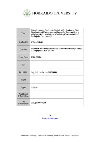
Figure 127 shows a graph of G1(M1) plotted against Ml for several values of
b. It is to be noted that G1(M1*)=lje =0.368. Therefore the probability
that the magnitude of the largest earthquake exceeds Ml* is 0.632.
G(M,)
Of.
99
98
95
90
85
80
70
60
1/ I /
I
,t7/ / ) /-Q ,.
II /~ /
II / / ()¥
1/ / /' /
//// /
f-- '---- 11///
11///
50
40
fW/ I
- - '--
30
dJ
20
10
5
O.
r-I-;~~
:6VMiM~-1 M",
..
I I I I L I I I
M,
Fig. 127. Graph of G1(M1), the probability that the magnitude of the largest earthquake
is equal to or less than M l'
Equation (152) or (153) is a case that has been treated in Gumbel's
theory of extreme values.336) These equations, or similar equations for
maximum acceleration or seismic intensity at a certain site, have been used
for estimating earthquake risk337)-342) usually under the assumption of
stationary random occurrence of earthquakes in time.
The probability that the ith largest earthquake has a magnitude between
M; and M;+dM; and the jth largest earthquake (i<j) has a magnitude
between Mj and Mj+dMj is given by

386 T. UTSU
b'2 ij
g;j(M;,Mj)dM;dMj = (i-I)! (j-i-I)! lO-jb(M;-M;*)lO<i-;)b(Mi-Mj)
X (l-lO-b(M;-Mj)}j-;-l exp {_ilO-(Mj-M/)} dM;dMj . (154)
The probability that M;-Mj has a value between x and x+dx is given by
b'(j-I) !
q··(x)dx- lO-;b%(I-lO-b%)j-i-ldx. (155)
'I - (i-I)! (j-i-I) !
This is a beta distribution as to
z = I-IO-h . (156)
The probability that M;-Mj is smaller than x is given by
%
Q;; = Jq;j(x) dx = E. (j-i, i) IE (j-i, i) (157)
o
where E. and E denote an incomplete beta function and an ordinary beta
function respectively. Equation (157) was used in estimating the accuracy
of b-value determinationY5) It was found from this equation that a previous
discussion on the accuracy of b-value (Utsu,l) p. 594) was incorrect.
13.3 Estimation of b-value and its accuracy
The value of b in equation (1) or (144) for a given group of earthquakes
was determined usually from the slope of a straight line fitted to the plotted
points on a log n(M) vs M diagram by the method of least squares. However,
such determination of b-value may be subjected to the following criticisms.175)
(1) The assumption the method of least squares is based on is not
valid for this kind of distribution. Moreover, the ordinary least squares
method gives too heavy weight to the points for large magnitude. Utsu,
175),176) using Monte Carlo technique, showed that the ordinary least squares
method yields systematically small b-values when the total number of earth-
quakes is small (less than about 400). Deming's method of least squares343)
with proper weighting gives more accurate and unbiased b-values.
(2) Different b-values are obtained according to the choice of the length
of interval 11M of magnitude in classifying earthquakesl84),344) and also the
treatment of the data in the magnitude intervals for which observed frequency
of shocks is zero. The points representing n(M)JM=0 can not be plotted
on the semi-log diagram, but if these points are neglected, unreasonably low

Aftershochs and Earthquahe Statistics 387
b-values are sometimes obtained, especially when the total number of
earthquakes is small. Such determination may lead to a misleading conclu-
sion that the b-value increases with increasing number of earthquakes.
Utsu176).192) recommended the following simple formula, because it gives
unique, unbiased, accurate estimate of b-values.
b = __ slog e __
"L.M,-sM,
(158)
where "L.M, is the sum of magnitude of all earthquakes having magnitude equal
to or larger than M, and s is the total number of these earthquakes. (Note
that M,=Ms'-(JM/2), if magnitude values are given at intervals of JM,
and Ms' is the central value of the lowest magnitude class). This equation has
been derived by equating the first-order moment for the samples "L.(M,-M,) to
that for the population r(M-M,)n(M)dM =(s log e)/b. Aki345) pointed out
Ms
that this is the same as the maximum likelihood estimate of b and tabulated
the confidence limits of b-value for large values of s (s250). The value of M1*
can be estimated from
M1* = (log s)/b-M,. (159)
Utsu177 ) has shown that the probability density function of b-value
determined from equation (158) is given by
. s' ( bo )'+1 ( SbO ) dbf(b)db=--- - exp - - -
r (s) b b bo
(160)
where bo is the value of b in the population. Cumulative distributions of
b/bo and bo/b have been plotted for various values of s from 7 to 3000.
From these graphs we can estimate the accuracy of b-value determined by
this method. The statistical test for the difference in b-value between two
groups of earthquakes A and B can be made by use of the F-distribution,
since bB/bA. has an F-distribution with 2sA and 2sB degrees of freedom (suffixes
A and B indicate groups A and B respectively and it is assumed that bjl <bB),
if there is no difference between the" two groups.
The value of magnitude is usually given to the one-tenth of the magnitude
unit, i.e., it is given at intervals of JM =0.1. In some cases, however, the
interval is 1/4 or 1/2. It has been pointed out that the estimate of b-value
is dependent on this interval. Utsu176) showed that the maximum likelihood
estimate of b is systematically small, when the interval is large. The value

388 T. UTSU
calculated from equation (158) should be corrected for this bias, if bt1M is
larger than a certain value. The correction 7] has been obtained as follows.
The probability that the magnitude M of an earthquake falls in the range
between jt1M+M, and (j+l)t1M+M, (j=0, 1,2, .... ) is given by
p; = (l_lO-b.dM) lO-b;AM . (161)
Therefore, the mean and the variance of M -M, are given by
00 ( . 1) (lO-bAM 1)/11 = j~P; J + 2 JM = 1-lO-bAM + -2 t1M, (162)
and
(163)
s
respectively. Then the mean and the variance of 2:: (Mi-M,) are S/11 and
i-I
S/12 respectively. Consequently, the b value corresponding to the mean of
s
2:: (Mi-Ms) becomes
i-I
b= S (log e) j (S/11) = bj7] (164)
where
(
lO-b.dM 1 )
7] = l_lO-bAM + 2 bt1Mjlog e . (165)
Thus, the b value calculated from equation (158) should be multiplied by 7] to
obtain an unbiased estimate. 7] is tabulated in Table 18 as a function of
MM. It is seen from this table that no correction is necessary when bt1M is
less than about 0.2. The value of b in the expression of 7] should be the value
for the population which is unknown to us, and we inevitably use its estimated
value. This substitution causes a decrease in accuracy with increasing bt1M,
though the variance of the b value from equation (158) decreases with increas-
ing bt1M as given by
v = __8_/1_2_ = __4_<_1O_-_b-:-.d_M-'-c)_
(S/11) 2 S (1 +10-b.dM) 2
(166)
Table 18. Correction TJ as a function of bAM.
bAM I 0.0 I o. 1 I o. 2 I o. 3 I o. 4 I o. 5 I o. 6 I 0.7 I O. 8 I o. 9 I 1. 0
TJ 11.000 11.00411.017 11.03911.070 11.10811.154 11.20811.26811.344 11.407

13.4 b-values for various seismic zones and their redeterminations
More than 250 papers are known to the author which include descriptions
of b, m, or y values for earthquakes occurring in some regions of the world.
Figures 128 and 129 show the frequency distributions of band m values for
shallow earthquakes reported in these papers. Some determinations using
apparently inadequate data are not included. When many b-values have
been determined for the same region for different time intervals in the same
paper, only one representative value for the entire period is adopted. Due
to the wide variety of the quality of data and the biased sampling of the regions
investigated, these graphs are only a rough indication of the scatter of band
m values.
/00
Freq.
50
Af tershocks. foreshocks
swarms

'-
oL---~~~--------~---------L~~~~
0.5 /.0 1.5 2.0
b
Fig. 128. Frequency distribution of b-values published in seismological literature.

390
50
Freq.
/
A /
/
/
/
T. UTSU
All types
Aftershocks. swarms
(including volcanic shocks)
Volcanic shocks only
/ ' /
./~/"-"."::...:------OL-__~?2-~~~~______~~__~~~~__-2~
1.0 1.5 2.0 2.5 3.0
m
Fig. 129. Frequency distribution of m-values published in seismological literature.
In Figures 128 and 129, solid lines indicate frequencies of band m-values
for all types of earthquakes including the values for aftershock sequences,
swarms, volcanic earthquakes, etc. Broken lines indicate those for after-
shock sequences, foreshocks sequences, and swarms including volcanic
earthquakes. Dotted lines in Figure 129 represents volcanic earthquakes only.
The medians of b-values for general earthquakes (excluding the values for
aftershock sequences, etc.) and for aftershock sequences, foreshock sequences,
and swarms are 0.96 and 0.85 respectively. The former value is nearly equal
to the b-value for Japanese shallow earthquakes and the latter value is equal
to the median of b-value for Japanese aftershock sequences (Chapter 5). The
median of b-values for all types of earthquakes is 0.89. The medians of m-
values for all types of earthquakes and for aftershock sequences, foreshock
sequences, and swarms are both 1.85. Most of the m-values have been
determined generally for earthquakes of smaller magnitude than earthquakes
for which the b-values have been obtained.
The main reasons for the variability of b-values are attributable to the
following causes.
(1) Actual variation in the magnitude-frequency relation among various
regions, time intervals, and magnitude ranges.
(2) Choice of the magnitude scale or the seismographs on which the
magnitude or amplitude values are dependent.
(3) Errors in the determination of b or m-values due to i) incompleteness
of data, ii) inadequacy of the method used in the determination, and iii)

random sampling fluctuations of purely statistical nature. Some probable
cause of the incompleteness of data will be described in Section 13.5 (p. 416).
Some of the papers reporting b-value determinations contain tables listing
the frequency of earthquakes of each magnitude interval or the magnitudes
of individual earthquakes. For such groups of earthquakes b-values have
been recalculated by using equation (158). Most of the recalculated values
do not differ much from the values given in the original papers, but in some
cases the recalculated values differ to such an extent that the conclusions of
the original papers have been modified. In this section these recalculated b-
values are presented together with some comments on the data and the con-
clusions found in respective papers. The recalculated values and the total
number of earthquakes used in the calculation are denoted by 6 and s
respectively, while the values found in the original papers is denoted by b.
i) Worldwide studies-shallow earthquakes
It should be noted that a comparison of b-values among various seismic
regions is meaningful only when the data are based on the same magnitude
system.
In their book "Seismicity of the Earth", Gutenberg and Richter319)
reported b-values for various regions of the world. The time intervals from
which the data have been taken differ with magnitude ranges. The intervals
are 1904-1945 (42 years) for M27 3/ 4, 1922-1945 (24 years) for 7s;.Ms;.7.7,
and 1932-June 1935 (3 1
/ 2 years) for 6s;.Ms;.6.9. Some earthquakes outside
of these intervals of time and magnitude are listed in their book, but the
complete listing is confined to the above intervals. For southern California
and New Zealand, however, b-values have been determined for earthquakes
with ML24 occurring during 1934-May 1943 and October 1940-January
1944, respectively.
6=0.78 (s=54),
6=0.93 (s=471),
6=0.92 (s=59),
6=0.73 (s=39),
6=0.93 (s =236) ,
6=0.96 (s=23),
6=0.93 (s=54),
6=0.78 (s=101),
6=0.76 (s=32),
Regions 1,2, Aleutian, Alaska, Brit. Col., b=l.l±O.l,
Southern California, ML24, b=0.88±0.03,
Regions 5, 6, Mexico, Central America, b=0.9±0.1,
Region 8, South America, h<lOO km, b=0.45±0.1,
New Zealand, M L24, b=0.87±0.04,
Region 12, Kermadec and Tonga Is., b= 1.3±0.2,
Region 15, Solomon to New Britten Is., b=l.OI±O.07,
Region 19, Japan to Kamchatka, b=0.80±0.08,
Region 24, Sunda Are, b=0.9±0.1,

392
b=0.81 (5=29),
b=0.72 (5=15),
b=l.41 (5=23),
b=l.30 (5=19),
b=0.95 (5=9),
b=l.28 (5=8),
T. UTSU
Regions 26, 28, Pamir-Eastern Asia, b=0.6±0.14,
Region 30, Asia Minor-Levant-Balkans, b=0.9±0.1,
Region 32, Atlantic Ocean, b=I.4±0.2,
Region 33, Indian Ocean, b=1.3±0.1,
Region 43, Southeastern Pacific, b= 1.1±0.2,
Region 45, Indian-Antarctic Swell, b=1.06±0.03,
and for the world's shallow earthquakes
b=0.84 (5=804), the whole world, b=0.90±0.02.
These b values, except three oceanic regions 32, 33, and 45, do not differ
largely from the value for the whole world. If these three oceanic regions
are combined, we obtain
b=l.37 (5=50), Regions 32,33,45.
This value is higher than that for the whole world. Two high b-values of
1.6±0.2 for region 40 (Arctic Ocean) and 1.8±0.2 for region 44 (East Pacific)
are included in the first edition of "Seismicity of the Earth", but no data are
available from this book for recalculation.
On the basis of the b-values found in this book and in some other papers,
Miyamura346).347) emphasized the regional variations of b-value and their
relation to the regional tectonics. Chouhan et al.333) also calculated a and
b values for 37 regions from the data found in the same book. The b-values
obtained by them ranges from 0.35 to 1.42 with a median of 0.79. Accuracy
of these values is probably low, because of the small number of data and the
incompleteness of the Gutenberg-Richter's catalog for the time intervals and
magnitude ranges adopted by Chouhan et al.
Duda348) prepared a catalog of world large earthquakes for the period
1897-1964, and calculated b-values for seven regions of the circum-Pacific belt
using the data for M':2:.7 in the years 1918-1963. The recalculated b-values
for shallow earthquakes (h::::;;65 km) are as follows.
b=0.93 (5=50), Region 1, South America, b=0.91±0.09,
b=1.13 (5=60), Region 2, North America, b=1.33±0.08,
b=1.36 (5=40), Region 3, Aleutians, Alaska, b=0.73±0.08,
b=1.03 (s =87) , Region 4, Japan, Kuriles, Kamchatka, b=1.01±O.05,
b=1.14 (5=105), Region 5, New Guniea, Banda Sea,
Moluccas, Philippines, b=1.24±0.07,
b=1.32 (5=112), Region 6, New Hebrides, Solomon,

New Guniea, b=l.42±0.10,
b=l.l1 (s=26), Region 7, New Zealand, Tonga,
Kermadec, b=l.00±0.06.
The recalculated values are in approximate agreement with those given by
the original author except for region 3. The magnitude distribution for this
region is shown in Figure 130. Straight lines fitted by the least squares method
and the maximum likelihood method are drawn in the figure. The least
squares method seems to weight three large shocks (N: 8.7, 8.6, and 8.2) too
heavily. An F-test has shown that there are no significant differences III
b-value between these seven regions at a significance level of 0.02.
100
Region 3
N
10
8
M
9
Fig. 130. An example showing the large difference between b-values estimated
by the method of least squares (LSE) and by the method of max-
imum likelihood (MLE). Data taken from Duda.347)
Tomita and Utsu349) used the magnitude given by U.s. Coast and
Geodetic Survey for shallow earthquakes (h:o:;;:100 km) of magnitude 5 and
above occurring in three years from 1964 through 1966, and obtained the
maximum likelihood estimates of b for 41 regions of the world. Gutenberg-
Richter's division319) of the world into 51 regions are adopted without modi-
fication, but in ten regions the b values have not been estimated since less than
ten earthquakes occurred during these years. The b-values obtained ranged

394 T. UTSU
0
0
0
0
0
Region A (I) 0 Region B ( 2.3.4.5)0
b ; 1.19 0 b ; 1.150
MM) 0 0
0 •
• •
•• ••• •• ••00 0
•• •
•• •
•••
I I
5 6 7
M
5 6 7
•Region C (6.7) 0 Region D (8.9)
•b ; 1.16
• b ; 1.06
• ••0
•
• •
•
0 ••
•• •• ••
••
•••••
I 1
5 6 7 5 6
•
•100-
Region E (f0) • Region F ( 12)
·0
b 0.75 • 1.34• ;
b ;
• •• •
• ••
• •
• •
••
• ••
6 7
1~5----------~6--~~----~7~
Fig. 131. N(M) plotted against M for fifteen regions using CGS magnitude for the
and Richter. 319) Taken from Tomita and Utsu. 34SJ

•••
•
• Region G (13,14,15,16)
•••
•
b ~ 0.98
•••
•
•
•
•
Region H m: 18,20)
• b' 1.20
••
•
•••
•
••
•••
•••
••
•
•
Region I (19)
b ~ 1.13
•
•
•
•
•
15~----------~--------~~~15~--------~6------e-15~----------~6--~O--
••
•
•
395
•
Region J (21,22,23)
b = 0.88
•
• •
•
Region K (24)
b = 1.03 •
•
Region L (25, 26,27. 28)
b = 0.89
•
•
•
••
•
•••
•
1~5----------~6--------~~
••
Region M (29, 30)
b = I, 14
••
•
•
••
•
•
•
•••
•
•
•
•
•
•
•
•
•
•
•
•
1~5----------~6--'---15~--------~-----------!'
•
••
Region N (32,33,45)
b = I. 09
•
•
•••
••
•••
•••
••
•
•
Region 0 (43,44)
b = 1.36
•••
••
••
1~5--------~6~-'----- 1·5~---------~6:-----------c!7 I,L
5
----------.l6
--------
years 1964-1966. Numerals in parentheses indicate the regions defined by Gutenberg

396 T. Drsu
from 0.60 to 1.40 with a median of 1.08. The b-value for all shallow earth-
quakes in the world was estimated as 6=1.07 (s=3170).
To reduce the errors due to the smallness of the data size, some of the
adjoining regions with approximately equal b values have been grouped
together. Figure 131 shows the plots of log N(M) against M for the fifteen
regions A, B,... , 0 thus defined. The numbers in parentheses in each graph
indicate the region numbers defined in Gutenberg-Richter's book. The
maximum likelihood estimates of b are also shown in each graph. These
estimates scatter in the range between 0.75 and 1.36. The lowest value of
0.75 for region E (South Atlantic Ocean) might be caused by incomplete
listing of events for magnitude below about 5.5. The significance of the
difference in b value between these regions have been tested by using the F-
distribution. The results are shown in Figure 132, in which crosses indicate
that the hypothesis of equal b-values for the two regions concerned can not
be rejected at a significance level of 0.1. Single and double circles indicate
that this hypothesis can be rejected at significance levels of 0.1 and 0.02
respectively.
Among a total of 105 combinations of two regions from fifteen regions,
-
A
Xrg
X X C
X X X 0
@ 0 0 0 E
X X X X @ F
0 X X X 0 @ G
X X X X @ X X H
X X X X 0 X X XI
@ X X X X @ X 0 0 J
X X X X X X X X X X K
0 X X X X @ X 0 X X X L
X X X X 0 X X X X X X X M
X X X X 0 X X X X X X X X NI
X X X X @ X 0 X X @ X 0 X Xlol
Fig. 132. Significance of the difference in b-value between every pair of the regions
A to O. Single and double circles indicate the difference at significance
levels of 0.1 and 0.02 respectively.

23 and 9 combinations having significantly different b-values are found at
the above two significance levels. However, if region E is excluded because
of lack of accuracy, 12 and 5 combinations among a total of 91 combinations
have significantly different b-values at the same significance levels. Consider-
ing that the ratios 12/91 and 5/91 do not differ largely from 0.1 and 0.02
respectively, it is difficult to draw a conclusion about the regional difference
in b-values from these data.
Miyamura350) reported b-values for various regions of the circum-Pacific
zone on the basis of the CGS magnitude data in the year of 1965. He stated
that the results showed a similar tendency to those found in his previous
studies.
ii) European regions
Bath351) obtained a fairly small b-value for Fennoscandia using
macroseismic data during 1891-1930. The maximum likelihood estimate for
shocks of magnitude 2.5 and above is
h=0.50 (5=343), Fennoscandia, M:::o:2.5, b=0.46.
Utsu176) considered that this small b value might be due to the magnitude
scale Bath adopted. However, Miyamura352) opposed to this view.
Miyamura,353) using Bath's data, calculated and compared b-values for
five regions of Fennoscandia. Each region has a small b-value in the range
from 0.47 to 0.61.
Karnik10),354) estimated the magnitudes of many earthquakes in Europe
from seismic intensities and obtained b-values for 39 regions on the basis of
these magnitude data. The values ranged from 0.5 to 1.1 with a median of
0.83. The recalculation is performed for the following eight combined regions
for which Karnik also gave b-values in his paper.
b=0.85 (s=125), Regions 1,2, Iceland and vicinity, M:::o:4.7, b=0.79,
b=0.65 (s=91), Regions 3, 10, Fennoscandia to England,M:::o:4.1, b=0.96,
b=0.94 (s=85), Regions 5-9,11, White Russia to France, M:::o:4.1, b=0.84,
b=0.75 (s=320), Regions 13-16, South of Mediterranean, M:::o:4.1,
b=1.01,
b=0.90 (s=1525), Regions 17-22, East Spain to Rumania, M:::o:4.1,
b=1.01,
b=0.72 (s=456), Regions 23, 24, 27, 33, 34, NW Iran to Bulgaria,
M:::o:4.7, b=0.64,

398 T. UTSU
b=0.97 (s=117), Regions 28,32, Northeast of Black Sea, M?:.4.7,
b=0.97
b=1.00 (s=94), Regions 30,31,35-39, Turkey to Libya, M?:.5.2,
b=l.15.
No simple relationship is evident between the b-value and the tectonic type
of the region as Karnik mentioned.
Niklova and Karnik335) reported b-values for 19 regions in and near the
Balkans from data on earthquakes of M?:.4.1 or M?:.4.6. The values ranged
from 0.53 to 1.10 with a median of 0.76. Frequencies of earthquakes as a
function of magnitude have been reported for Greece by Galanopoulos,356)
for Turkey by Ocal,357) and for Bulgaria by Grigorova et al.358) The
maximum likelihood estimates of b for these regions are as follows.
b=0.65 (5=1613), Greece, 1840-1959, M?:.4.8,
b=0.45 (s=1499), Turkey, 1850-1960, M?:.3.5,
b=0.60 (s=124), Bulgaria, 1901-1965, M?:.4,
b=0.69,
b=0.58.
In a later paper Galanopoulos359) adopted b=0.82 for the region of Greece.
iii) North America
As already mentioned the first b-value found in seismological literature
was b=O.88 for southern California.314) Allen et aJ.292) obtained b-values for
six regions in southern California in the magnitude range 3 and greater. These
values are not much different from the above value of 0.88. The lowest value
is found for Kern County (b=0.80) and the highest value for Los Angeles
Basin (b=1.02). Niazi360) obtained b=0.99 for earthquakes with M?:.4 in
northern California and western Nevada. Ryall et aJ.361) constructed magni-
tude-frequency graphs for six regions in the western United States. The
b-value for the period from 1932 to 1962 for magnitude 4 and greater are 0.61,
0.63, 0.68, 0.79, 0.79, and 0.90. Ryall et al. suspected that the first three
low values are the results of poor detection of small shocks. Duda362) report-
ed the following b-values: b=0.47 (2.7:=;:M:=;:3.6) and b=l.11 (3.7:=;:M:=;:4.5)
for Baja Claifornia, b=0.46 (2.0:=;:M:=;:4.2) and b=1.07 (3.8:=;:M :=;:4.6) for
Imperial County, California, and b= 1.21 (1.5sM s2.1) for Arizona.
Evernden363) obtained b= 1.29 for earthquakes in the USA using CGS
magnitude data from 1961 to August 1968. His paper includes b-values
for various regions of the world published by other investigators.
The following b-values are obtained from the data by Milne.364)

b=0.75 (s=435), Aleutians, 189~1960, M~6,
b=0.49 (s=181), Western Canada, 189~1960, M~5,
b=0.80 (s=65), Eastern Canada, 1898-1960, M~5,
b=0.89,
b=0.67,
b=0.78.
399
In addition to these determinations, b-values have been reported for
several aftershock sequences and swarms as described in sub-section vii).
iv) Japan and vicinity
Kawasumi31B
) determined the value of bK in equation (124) for Japanese
earthquakes from data for 40 years from 1904 to 1943. The maximum
likelihood estimate from the same data is
bK =0.52 (s=343), Japan, MK~4, bK=0.537.
From equation (126), this corresponds to the b-value of 1.04.
Tsuboi365 ) in 1952 first described the regional difference in b-value in
Japan using data on earthquakes with magnitude 6 and above occurring
during 1931-1950. The b-values determined by the method of least squares for
three regions A, B, and C differ considerably (see below). However, recal-
culated values using the same data do not show any appreciable differences.
b=0.96 (s=292), Region A, Pacific Ocean side of NE Japan,
b=0.94 (s=90), Region B, Pacific Ocean side of SW Japan,
b=0.96 (s=65), Region C, Japan Sea side of the whole Japan,
b=1.06,
b=O.72,
b=0.66.
Tsuboi also calculated b-values for the whole of Japan as a function of the
length of time interval. The result indicated clear depencence of b-value
on the length of time interval, i.e., on the number of earthquakes used in the
calculation. The b-value increases with the length of time interval and
reaches a constant value asymptotically. However, maximum likelihood
estimates on the basis of the same data do not show such a tendency. The
method of least squares adopted by Tsuboi yields small b-values when the
size of data is small. For example, Tsuboi gave a very small value of b=
0.21 for the year of 1950, but the recalculated value for this period is b=1.15
(s=15).
Tsuboi366 ),367) in 1957 and 1964 calculated b-values for shallow earth-
quakes occurring in and near Japan. The recalculated values using the same
data are as follows.
b=0.81 (s=382), In and near Japan, 1931-1955, M~6,
b=1.03 (s=433), In and near Japan, 1926-1963, M~6,
b=0.72,366)
b=0.87,367)

400 T. UTSU
6=0.96 (s=1231), In and near Japan, 1885-1963, M;;;:.:6, b= 1.03.367)
Usami et al.258) obtained b=1.18 for earthquakes of M;;;:.:6 at all depth
ranges in and near Japan during 1926-1956. The recalculation has been
made for earthquakes of focal depths 60 km and less, since the magnitudes of
earthquakes deeper than 60 km have been provided from different sources.
6=1.00 (s=340), In and near Japan, h:s;;:60 km, M;;;:.:6.
In their paper, b-values are also shown for two focal depth ranges 0-30 km
and 30-60 km. Recalculated values are
b=0.90 (s=185), In and near Japan, 0:s;;:h:s;;:30 km, M;;;:.:6,
6=1.15 (s=155), In and near Japan, 30<h:s;;:60 km, M;;;:.:6,
b=0.92,
b=1.25.
These values are nearly equal to those obtained by Hamamatsu,186) since
the materials are mostly the same.
Hamamatsu,186) giving due consideration to the limitation of the
materials, calculated b-values for Japanese regions for two depth ranges.
Recalculated values are as follows.
6=1.02 (s=363), The whole Japan, 0:s;;:h:s;;:60 km, M;;;:.:6,
6=0.93 (s=204), The whole Japan, 0:s;;:h:s;;:30 km, M;;;:.:6,
6=1.17 (s=159), The whole Japan, 30<h:s;;:60 km, M;;;:.:6,
6=1.04 (s =278) , NE Japan, 0:s;;:h:s;;:60 km, M;;;:.:6,
6=0.89 (s=139), NE Japan, 0:s;;:h:s;;:30 km, M;;;:.:6,
b=1.16 (s=139), NE Japan 30<h:s;;:60 km, M;;;:.:6,
6=0.95 (s=84), SW Japan, 0:s;;:h:s;;:60 km, M;;;:.:6,
b=0.95 (s=64), SW Japan, 0:s;;:h:s;;:30 km, M;;;:.:6,
6=1.32 (s=20), SW Japan, 30<h:s;;:60 km, M;;;:.:6,
b=1.07,
b=1.00,
b=1.13,
b=1.10,
b=1.05,
b=1.10,
b=0.89,
b=0.83,
b=1.21.
The two values 6=0.93 and 6=1.17 for the two depth ranges for the whole
Japan differ significantly at a significance level of 0.1.
Katsumata187) determined b-values for several selected regions of high
seismic activity in and near Japan. He prepared additional materials to the
JMA catalog of earthquakes (supplementary volumes of the Seismological
Bulletin of JMA) in order to avoid the inaccuracy of b-values due to the use
of incomplete data. Erroneous b-values had been obtained in several papers
of different authors who used the JMA catalog without proper consideration
to its limitations. Katsumata368) later recalculated the b-values for the same
region using equation (158). Some of the recalculated values are listed below,
together with the values from the old paper.

b=1.03 (s=213), Off the Pacific coast of N Honshu, M:::::6, b=1.07,
b=O.88 (s=146), S Hokkaido and off the coast of
S Hokkaido, M:::::5, b=0.89,
b=1.03 (s=238), Kwanto district including nearby
sea areas, M:::::4.5, b=0.99,
b=0.95 (s=73), Kinki district and part of Shikoku
including sea areas, 4.5::;:M::;:5.5, b=0.95,
b=0.85 (s=78), Kyushu and off Pacific coast of
Kyushu, M:::::5, b=0.91.
Katsumata concluded that there are no remarkable differences III b-value
between these regions.
Ichikawa369) reported b-values calculated from equation (158) for the
following four regions. He tried three cases Ms =5.0, 4.8, and 4.6, but these
Ms values should be modified to 4.9, 4.7, and 4.5 respectively, since the
frequencies were given at intervals of 0.2 unit of magnitude. The recalculat-
ed values are as follows.
b=0.82 (s=234), Chubu district, M:::::5,
b=0.81 (s=134), Western Japan, M:::::5,
6=1.21 (5=62), SW Ibaragi Prefecture, M:::::5,
6=0.84 (5=37), Northern Chiba Prefecture, M:::::5,
b=1.17,
b=1.20,
b=1.67,
b=1.04.
It is concluded that earthquakes in SW Ibaragi Prefecture have a significant-
ly higher b-value than those in Chubu district and western Japan. Ichika-
wa232) discussed the b-values also for four regions in and near the Izu Peninsula.
Some of the b-values reported by Miyamura,247) by Maki,370) and by Welk-
ner371) seem too small. These authors used the ]MA catalog only. Welkner
determined the b-values by the least squares method and the maximum
likelihood method for earthquakes of magnitude 5.5 and above in nine regions
covering Japan and surrounding areas. The b-value ranged from 0.63 to 0.90.
However, the JMA catalog is far from being complete for earthquakes of
magnitude about 6 or less occurrring in the regions concerned. The similar
comment may be made on a value of b=0.72 for earthqaukes with M:::::5 in
the Hokkaido region published by the Sapporo District Meterorological
Observatory.372)
Ikegami325) determined the values of bI in equation (127) using mean
annual frequencies of felt shocks at each seismic intensity averaged for stations
in each of the three regions A, B, and C in Japan. The three regions are the

402 T. UTSU
same as those defined by Tsuboi.365) In calculating the mean annual
frequencies, Ikegami neglected the stations at which no felt shocks have been
registered at a given seismic intensity. For example, in the C region which
includes 27 stations, the seismic intensity 6 has been recorded only once at
one station during the 30 years investigated. He regarded the mean annual
frequency at intensity 6 in region C as 1/30, but this should be modified to
1/(30 X27). The recalculated values using the modified mean annual frequen-
cies do not show large regional variations in contrast with Ikegami's
conclusion.
61=0.50, Region A, Pacific Ocean side of NE Japan,
61=0.52, Region B, Pacific Ocean side of SW Japan,
61=0.44, Region C, Japan Sea side of the whole of Japan,
61 =0.49, Regions A, B, and C, the whole of Japan,
b1 =0.58,
b1=0.46,
bI =0.39,
b1=0.49.
Katsumata and Tokunaga326) obtained values of b1 for 64 stations in
Japan. The value varies from 0.44 at Toyooka to 0.93 at Wakayama with
a median of 0.61. No large-scale regional variations are evident.
v) Oceanic seismic belts
Sykes373) obtained a b-value of 0.91 for 267 earthquakes of M~4.0
occurring in the ridge system which extends from the the north Atlantic
to the Arctic during the years 1955 through 1964. The recalculation has been
done for M~4.5.
6=0.90 (s=101), Arctic region, M~4.5, (b=0.91).
From Stover's data for the Indian Ocean294) and the South Atlantic
Ocean,374) the following values are obtained in the recalculation.
6=0.97 (s=76), Indian Ocean, 1922-1951, M~6,
6=0.96 (s=83), South Atlantic Ocean, 1964-1966, M~4.7,
b=0.91,
b=1.04.
Francis375) studied the magnitude-frequency relation for earthquakes in
the mid-Atlantic ridge using magnitUdes determined by CGS from 1963 to
May 1967, and found that the b-value for earthquakes in the fracture zone
is normal (b= 1.03) whereas the b-value for earthquakes at median rift is high
(b= 1.73). He mentioned four possible interpretations for this difference:
(1) Focal mechanism, (2) temperature gradient, (3) volcanism, (4) systematic
error in the measurement of magnitude (see also Sykes376»)
For Hawaii, the recalculation yields the same value as found in the

original paper by Furumoto.293)
6=0.97 (s=976), Hawaii, 1950-Sept. 1959, M~2.5, b=0.97±0.064.
vi) USSR
In the USSR, the frequency distribution of earthquake magnitude is
usually represented by the y-value in equation (134). Most of the papers
dealing with y-values do not include tables showing the frequency of earth-
quakes in each energy class. The reported y-values (e.g., Bune,37'1) Fedotov
et al.,134).378) Gzovsky et al.,379) Riznichenko,380-382) Riznichenko and Ner-
sesov383) Tskhakaya,384») fall in the range. from 0.35 to 0.60, and the values
from 0.45 to 0.50 are most frequent. Kantorovich et al.385) obtained a
maximum likelihood estimate of y, Y=0.45 (s=707) for central Asia.
Some Soviet authors384),386),387) use b-values, too. Recalculated values
of y and b for earthquakes in the Caucasus376) are given below.
y=O.54 (s=1633), Caucasus, 1924-1960, K~lO,
6=0.90 (s=1435), Caucasus, 1912-1960, M~3.5,
vii) Other regions
b=0.89.
Sutton and Berg290) obtained a b-value for earthquakes in Western Rift
Valley of Africa from three-year observation. The recalculated value is
6=0.65 (s=234), Western Rift Valley, Africa, b=0.6,
In Sutton and Berg's paper, we find the following explanation for the low
b-value: "The observational radius of the African station decreases with
decreasing magnitude and the larger area is monitored for the large shocks
than the smaller shocks."
In Niazi and Basford's paper388) on seismicity of Iranian Plateau and
Hindu Kush region, a magnitude-frequency table is found for region C (the
belt surrounding the central desert of Iran).
6=0.65 (5=476), Belt surrounding the central desert of Iran, M~4.
Ram and Rathor389) reported b-values for three regions of India, b=
0.59 (Delhi and Himalayan region), b=0.74 (Assam region), and b=0.81
(Koyna region), but the accuracy of these values can not be inferred from
their paper (see also Ram and Singh,390) and Ram and Sriniwas391»).
Mei392) studied the seismicity of China and obtained fairly low b-values
(0.4 to 0.6) for six regions in China. For the whole of China excluding

404 T. UTSU
Taiwan, the recalculated value from the data for fifty years IS
b=0.59 (s=311), China, M~5.5, b=0.57.
Keimatsu393 ) studied earthquakes of China III Ming (1368-1644) and
Sing (1644-1911) dynasties. Using his catalog of earthquakes in which
magnitudes have been estimated from macroseismic effects, the b-value has
beeen calculated.
b=0.53 (s=87), China, 1368--1911, M~7.0,
b=1.OO (s=62), China, 1368--1911, M~7.6.
For the New Guinea-Solomon region, the following b-value is obtained
from data in Denham's paper.394)
b=1.04 (s=549), New Guinea-Solomon, 1963-1966, M~5, b=1.l6.
Welkner395) obtained maximum likelihood estimates of b for each area
of lax lain northern Chile from the CGS epicenter and magnitude data for
1963-1966, and attempted to compare the b-value with tectonics. The
estimated values scatter very widely from 0.46 to 3.95 with a median of 0.85.
The smallness of the data size may account for such a wide scatter.
vii) Aftershock sequences and earthquake swarms
b-values for aftershock sequences and earthquake swarms are listed in
Tables 4 and 5 (Chapter 3). The b-values for Japanese aftershock sequences
and swarms listed in Table 4 have been determined on the basis of magni-
tudes calculated from Tsuboi's formula. 396) The median of these values is
0.85, which is somewhat smaller than the value of about 1.0 for general
earthquakes (including aftershocks, etc.) of magnitude 6 and larger in the
Japanese region obtained by several investigators1 ),186),188),367),368) who used the
JMA magnitudes calculated from Tsuboi's formula.
The values for m in Ishimoto-Iida's formula for aftershocks, especially
micro-aftershocks have been determined in the case of some Japanese earth-
quakes (see Table 7 in Chapter 5). The median of the m-values is about 1.85.
Some of the b-values reported for aftershock sequences and swarms in
California are fairly small. The maximum likelihood estimates of b have been
obtained for several sequences176) using data given by Richter et a1.122) (after-
shocks of the Desert Hot Springs earthquake of December 4, 1948; earthquake
swarm near Kitching Peak, June 10, 1944), Richter123) (aftershocks of the
Kern County earthquake of July 21, 1952), Tocher127) (aftershocks of the San

Francisco earthquake of March 22, 1958), Richter178) (earthquakes near China
Lake, January 7-16,1959), Udias133),397) (aftershocks of the Salinas-Watsonville
earthquakes of August 31 and September 14, 1963), and McEvilly et a1.64)
(foreshocks and aftershocks of the Parkfteld earthquake of June 28, 1966)
are as follows.
b=1.00 (s=89),
b=0.68 (s=44),
b=0.84 (s=200),
b=0.74 (s=182),
b=0.36 (s=81),
b=0.58 (s=54),
b=0.46 (s=35),
b=0.47 (s=45),
b=0.93 (s=18),
b=0.85 (s=22),
b=0.75 (s=224),
Aftershocks, Desert Hot Springs, M?:3.0,
Kitching Peak Swarm, M?:3.0,
Aftershocks, Kern County, M?:4.0,
Aftershocks, San Francisco, M?:2.0,
China Lake swarm, M?:O.O,
1/ M?:0.8,
Aftershocks, Watsonville (Aug. 31),133) M?:1.0,
1/ (Sept., 14),133) M?:1.0,
1/ (Aug. 31),397) M?:2.0,
1/ (Sept. 14),397) M?:2.0,
Parkfield sequence, M?:2.0
b=0.49,
b=0.41,
b=O.84,
b=0.63.
The values of b=0.53 for the aftershock sequence of the earthquake near
Corralitos on November 16, 1964 reported by McEvilly,137) b=0.78 for the
foreshock-aftershock sequence of the earthquake near Antioch on September
10, 1965 by McEvilly and Casaday,140) and b=1.40 for the microaftershocks of
the Truckee earthquake of September 12, 1966 by Greensfelder,140) are listed
in Table 5. In addition, Ryall et a1. 65) reported a value of b=0.81 for the
Truckee sequence and Fitch398) reported b=0.59 for microaftershocks of the
Parkfield earthquake.
Eaton et al.399) made a detailed study of the aftershocks of the Parkfield
earthquake and obtained b-values for various ranges of focal depth in two
sections of the hypocentral zone. From the list of aftershocks for July 11 to
September 15, 1966 in their paper, we obtain the following maximum likelihood
estimate of b.
b=0.88 (s=67), Aftershocks, Parkfield, M?:2.0, b=0.85.
Ranal1i400) calculated the maximum likelihood estimates of b for fifteen
aftershock sequences using data published by various authors.9),62),64),66),
122).126..127),133),282) These sequences include six Californian sequences, five of
which have been treated above. For the aftershocks of the Long Beach
earthquake of March 10, 1933, he gives b=0.79 (s=78).
Fairly large b-values of 1.5 and 1.45 have been reported for the aftershock

406 T. UTSU
sequences of the Kamchatka earthquake of 1952 and of the Aleutian earth-
quake of 1957 by Blith and Benioff125) and by Duda126) respectively. These
values are based on the so-called body wave magnitudes. Renalli400)
recalculated the b-value for the Aleutian sequence and obtained 6= 1.277 (s =
205). Utsu57) obtained b=0.70 for the same sequence on the basis of surface
wave magnitude converted from body wave magnitude by using Gutenberg-
Richter's formula. Utsu57) also obtained b=0.93 and b=0.88 for the after-
shock sequences of the central Alaska earthquake of 1958 and of the southeast
Alaska earthquake of 1958, respectively. Page62) obtained the maximum
likelihood estimate of b, 6=0.88 (s=293) for the aftershocks of the Alaska
earthquake of March 28, 1964 on the basis of body wave magnitude (4.5:5:
m:5:5.7). Ranalli400) reported 6=0.987 (s=294) for the same sequence on
the basis of Page's paper. Press and Jackson180) obtained b=1.1 for the same
sequence using amplitudes recorded by Wood-Anderson seismographs.
For the aftershocks of the southern Kurile Islands earthquake of October
13, 1963, the b-value is calculated using CGS magnitudes listed in a table
by Santo135) for the period from 09 h, October 13 through December 31.
6=1.15 (s=256), Aftershocks, southern Kurile Islands, m:::::4.5.
Two 6-values were reported by Motoya218) for the aftershocks of the
magnitude 7.8 earthquake on August 12, 1969 off Hokkaido, 6=1.07 for m:::::
4.6 using CGS magnitudes and 6= 1.44 for M:::::5.1 using JMA magnitudes.
Papazachos et al.9) studied many aftershock sequences in the region of
Greece, and obtained b-values for 29 sequences. The value ranged from 0.33
to 1.45 with a median of 0.73. Ranalli4°O) recalculated b-values for five of
these sequences. The values are 6=0.557 (s =85) for the Chalkidike sequence
of 1932 (b=0.52), 6=0.639 (s=299) for the west Thessaly sequence of 1954
(b=1.00), 6=0.926 (s=400) for the Amorgos sequence of 1956 (b=0.92),
6=0.905 (s=291) for the Magnesia sequence of 1957 (b=0.73), and 6=1.357
(s = 139) for the Zante sequence of 1962 (b = 1.07). He also obtained 6= 1.086
(s=103) for the Cremasta sequence of 1966 (b=1.12) studied by Comminakis
et al. 66) Drakopoulos and Srivastava401) obtained 6=1.25 (s=308) for the
aftershock sequence of the earthquake in Epidavros, Greece on July 4, 1968.
Gupta et al.402) obtained 6=0.56 (s =52) for the aftershock sequence of
the Godavari Valley, India, earthquake of April 13, 1969. Utsu175) obtained
b=1.22 for aftershocks of the great Outer Mongolian earthquake of December
4, 1957 from records of the Benioff short-period seismographs at College-
Outpost, Alaska.

From Duda's table129) for the Chilean earthquake sequence of 1960, the
b-value is recalculated as follows.
6=0.75 (s=110), Chile, May-December 1960, M L 5.8, b=0.7.
b-values have been obtained for some earthquake sequences in New
Zealand. Ranalli400) obtained 6=0.557 (s=71) for the aftershocks of the
Hawke's Bay earthquake of February 3, 1931. For the aftershocks of the
West Port earthquake of May 10, 1962, the following value is obtained from
the talbe of Adams and Le Fort. 59)
6=0.64 (s=71), Aftershocks, West Port, M L 3.0.
Hamilton58) reported a value of b= 1.05 for the foreshock-aftershock sequence
of the Fiordland earthquake of May 24, 1960.
viii) Variation of b-value with depth
According to Gutenberg and Richter319 ) b-values for the world's inter-
mediate and deep earthquakes are both b=1.2±0.2, which are somewhat
higher than the value for the world's shallow earthquakes (b=0.90).
Gutenberg403) developed the "unified magnitude scale". The b-values deter-
mined on the basis of this scale for the world's shallow, intermediate, and
deep earthquakes of magnitude above 7 are all 1.7, while the values for
earthquakes of magnitude between 6 and 7 are 0.92 (shallow), 0.54 (inter-
mediate), and 0.51 (deep).
Katsumata404) also determined and compared b-values for the world's
shallow, intermediate, and deep earthquakes. The recalculated values by
using equation (158) are
6=1.20 (s =804) , World's shallow earthquakes,
1950-1965, M L 6.5, b=1.23,
6=1.09 (s=195). World's intermediate earthquakes,
1950-1965, M L 6.5, b=1.14,
6=1.06 (s=73), World's deep earthquakes, 1950-1965,
M L 6.5, b=1.16.
No significant differences in b-value are found between these three groups of
earthquakes.
Tomita and Utsu349) described that the maximum likelihood estimate
of b for the world's shallow earthquakes of h::;:100 km (6=1.07, s=3170) is
approximately equal to that for the world's intermediate and deep earthquakes

408 T. UTSU
(b = 1.03, s=802) on the basis of CGS magnitude of m~5 in the years 1964-
1966.
Brazee and Stover405) calculated b-values for the world's shallow, inter-
mediate, and deep earthquakes on the basis of CGS magnitudes. The
result of recalculation using data on shocks of magnitude 5.4 and above is
as follows.
b=1.33 (s=861), World, 1964-1965, h<70 km, M~5.4,
b=1.27 (s=264), World, 1964-1965, 70::;:h::;:300 km, M~5.4,
b=1.38 (s=68), World, 1964-1965, h>300 km, M~5.4,
b=1.361,
b=1.124,
b=1.138.
The date reported by Rothe452) for the world's earthquakes yield the
following b-values.
b=1.11 (s=2060) , World, 1953-1965, h<70 km, M~6, b=1.22,
b=0.98 (s=517), 1/ 70::;:h<300 km, M~6,
b=1.04 (s=173), 1/ h::;:300 km, M~6.
No significant differences are evident between the three depth ranges.
Chohan and Srivastava406) investigated the variation of b with depth for
the world's earthquakes of magnitude 6 and larger based on the catalog in
Gutenberg and Richter's book.319) They found b-values of about 0.67 for
four depth reanges covering 0 to 400 km, and b= 1.09 for a range between 400
and 500 km, etc. These b-values, however, seem to be resulted from inade-
quate use of the catalog.
In the Japanese region, Katsumata199) obtained b= 1.2 for earthquakes
deeper than 150 km and b=1.1 for those deeper than 300 km. Later
Katsumata404) reported b-values of around 1.0 for shallow, intermediate,
and deep earthquakes in and near Japan. The recalcualted values are as
follows.
b=0.99 (s=356), In and near Japan, h<70 km, M~6.0,
b=1.02 (s=80), 1/ 70::;:h<300 km, M~6.0,
b=0.98 (s=78), 1/ h~300 km, M~6.0,
b=1.00,
b=1.07,
b=0.99.
Suyehiro,407) from a careful observation of small deep earthquakes at
Matsushiro, central Japan, showed that deep earthquakes of small magnitude,
say magnitude around 3, are not so frequent as expected from the frequency
of large deep earthquake of magnitude 6 or more. Thus the magnitude-
frequency relation is not represented by a linear equation of log n(M) and M.

Suyehir0408),409) obtained similar results for deep earthquakes In the Fiji
region and South America.
The b-values for intermediate earthquakes in the Hindu Kush region
have been described in several papers. The first b-value for this region is
b=0.6±0.1 given by Gutenberg and Richter.319) From Santo's paper41O)
on Hindu Kush seismicity, we obtain the following estimate of b.
6=1.41 (s=84),
6=1.25 (s=43),
Hindu Kush, h<100 km, m;:::::5.1,
" h> 100 km, m;:::::5.1.
Ram and Sriniwas391) showed a graph of logarithm of frequency versus magni-
tude for earthquakes in the Hindu Kush and Delhi region. The plotted
points lie on a straight line of slope 0.59 in the magnitude range from 2 to
more than 6 with unbelievably small scatter. It is also unbelievable that such
small earthquakes as of magnitude 2 or 3 have been observed without omission
in this region. Lukk20) obtained a high y-value for aftershocks of the Dzhurm
earthquake of 1965 (h=210 km) in the Hindu Kush region. Recalculation
yields the following value.
Y=0.66 (s=171), Aftershocks, Hindu Kush, K;:::::lO,
If shocks with K;:::::9 are used, },=0.58 (s=358).
y=0.87.
Another region of high seismic activity at intermediate depths IS the
Vrancea region in Rumania. Enescu and Jinau41I ) obtained b=0.70-0.75
for this activity. Constantinescu and Enescu412) reported that y=0.49 (K
;:::::10) and b=0.73 (M =3.5) for the Vrancea region. The recalculated y-
value is as follows (shocks of K = 10 are excluded).
y=0.60 (5=248), Vrancea, K;:::::11.
Radu and Tobias reported that the frequency of small earthquakes in the
Vrancea region with K <9 is fewer than that expected from the larger earth-
quakes.381) Purcaru21) obtained the b-value for the aftershock sequence of
the intermediate earthquake on November 10, 1940 in the Vrancea region.
On the basis of his paper we obtain
6=0.75 (5=35), Aftershocks, Vrancea, M;:::::3.9, b=0.71.
Galanopoulos413) reported b-values of 0.82 and 0.42 for shallow and inter-
mediate earthquakes in Greece, respectively. Tryggavason and Lawson414)
obtained b=0.57 for intermediate earthquakes near Bucaramanga, Colombia,
with body wave magnitude between 3.9 and 4.8 during 1962-February 1969.

410 T. UTSU
The earthquake frequency decreases more rapidly with increasing magnitude
in the range between 4.8 and 6.0.
As noted in a previous section, the b-value for Japanese earthquakes of
focal depths 0 to 30 km is somewhat lower than that of focal depths 30 to
60 km. Miyamura3(7) stated that in Japan b=O.7 ca. for crustal earthquakes
and b=0.9 ca. for subcrustal earthquakes. Parazachos et al.94
concluded
that the b-value for an aftershock sequence in Greece decreases with increasing
depth of the main shock as
b = 1.26-0.0135 h. 14 km::;::h::;::70 km (167)
It is well known that b-values are very high for some volcanic earthquakes
(for reviews of volcanic earthquakes, see e.g., Sakuma and Nagata,(15)
Minakami,(16) Kubodera417 »). These earthquakes are very shallow, less than
a few kilometers below the surface.
ix) Variation of b-value with time
In addition to the spatial variation of b-value, temporal variation of b
or m value has been discussed by several seismologists. Riznichenko382)
stated that the temporal variations of y exceed considerably the spatial
variations of time average of y.
Ikegami418) studied the variation of b-value with time during the recent
forty years for earthquakes in two sea regions A and B off the Pacific coast
of northeastern Japan. He used log LI as a measure of magnitUde, where LI
is the epicentral distance to the farthest station where the shock was felt.
On the basis of an empirical relation between log.:l and M, i.e., M =y' log LI-
8', he assumed a relation
log n (LI) = a'- (3' log LI (168)
where n(LI) is the number of earthquakes with maximum felt distance between
.:I-50 km and LI+50 km, and estimated {3'-values for each of the five-year inter-
vals starting from 1924, 1925, .. , 1960. The values of {3' vary considerably
with time with periods of 10 to 20 years in the both regions. The average
{3'-values are 2.67 for region A, 3.70 for region B, and 3.01 for region A+B.
Ikegami described that these values correspond to b-values of 0.99, 1.37, and
1.11 respectively, since {3'=by' and y' =2.7. However, the correct relation
is {3'=by' +1. Thus the b-values should be 0.62, 1.00, and 0.74 respectively.
The main reason for the small b-value for region A may be that many
earthquakes in this region occurred at places located more than 150 km from

the coast, while the statistics was taken for earthquakes with L1 150 km and
over. Many earthquakes having such mangitude that corresponds to L1 of more
than 150 km have not been included in the statistics as they were not felt in
Japan. Such earthquakes are more frequent in region A than in region B,
because the intense seismic activity spreads farther off the coast in region
A. Ikegami419),420) later studied the same problem by the same method for
several other regions and reached the conclusion that the b-value varies with
time in each region and the period of low b-value corresponds to the period of
high seismic energy release. This negative correlation between b-value and
energy release is naturally expected, even if earthquakes are random samples
from a population in which magnitudes are distributed in accordance with
Gutenberg-Richter's law with a time invariant b-value. For a group of
samples which includes large magnitude events by chance, the b-value
calculated by the ordinary least squares method is usually lower than the
value in population, since the method gives very heavy weight to a small
number of large events.
As described in Chapter 5, no significant variations of b-value with time
have been found in most aftershock sequences. The Matsushiro earthquake
swarm of 1965-1969 has been investigated in detail by many investigators.
b or m values have been reported for various stages of the activity and in
various magnitude ranges. The magnitude-frequency relation is normal for
the magnitude range between 4.0 and 5.1 on the basis of magnitude values
given by JMA, but earthquakes having magnitude larger than about 5.3 are
too few. 421). Okada422) obtained b=0.89 (s=230) for 4.0:::;:M:::;:5.5 for the
period from August 1965 through 1967. In this calculation equation (177)
was used together with an estimate of upper limit of the range M 1=5.5 from
the same equation. Okada also obtained b=0.43, b=1.13 and b=0.75 for
three periods, August 1965 to March 1966, April and May 1966, and June
1966 to February 1967, respectively. Katsumata36B ) obtained b=1.27 for
M~4.0 for the period from August 1965 through December 1966 without
setting the upper limit.
The Party for Seismographic Observation of Matsushiro Earthquakes
and the Seismometrical Section, ERp49) obtained m-values for every month
from October 1965 to February 1966 and for every ten-day intervals from
March 1966 to February 1967 from observations by acceleration seismographs
at three stations in the swarm area. The m-values at the three stations
show similar variations. The values were high (m=2.2-2.5) until February

412 T. UTSU
1966 and normal (m= 1.7-2.0) after March 1966. In the second decade of
January 1967, m-values were considerably low at the three stations. Hamada
and Hagiwara,350) and Hamada151) determined m-values for every ten-day
intervals for microearthquakes recorded at Hoshina in the swarm area.
Between February 1966 and May 1967 the m-value fluctuated in the range
from 1.4 to 2.6. In the periods of increased activity (April to June 1966, and
late August and early September 1966, and middle of January 1967), the m-
values were low, around 1.5, and in the other periods the values were about
2 or more. m and b values determined from the observations at the Matsushiro
Seismological Observatory did not exhibit such a tendency, though some
temporal variations were observed.152)
Drakopoulos et al.423) obtained b-values from observations of micro-
earthquakes at Suzaka and Matsushiro during three different intervals of the
swarm. They estimated the values from the slope of the log N(M) vs M
curves, but these curves were not correct since the data were lacking above
certain magnitude levels. The recalculation has been performed by using
equation (177).
b=0.66 (s=830), Matsushiro swarm, Suzaka, Dec. 20-26, 1965,
b=0.69 (s=515), II
b=0.50 (s=550), II
-O.4:o;:M:0;:1.1, b=1.05,
II May 13-14, 1966,
-0.5:o;:M:0;:0.8, b=1.19,
Matsushiro, May 21, 1966,
-3.2:o;:M:0;:-1.6, b=0.84.
Nishida424) made a seismic observation at Sanada near Matsushiro for
82 days in the summer of 1966 with a four channel recorder covering a dyanmic
range of about 60 db. He obtained m=1.267±0.04, m=1.877±0.153, and
m = 1.901 ±0.067 for the first, second, and third channels respectively. For
the fourth channel, which is of the lowest sensitivity, the number of recoded
shocks was too small to determine an accurate m-value. For the first
channel (the highest sensitivity) the variation of m with time is not remark-
able, but for the second and third channel, m values show appreciable temporal
variations in the range between about 1.6 and about 2.4. In late July and
early August m-values for these two channels are the lowest, while the
value for the first channel is the highest. In the first channel the average
frequency of recoded shocks was about 100 per hour. Such a high density
of shocks may cause considerable losses of small shocks by overlapping on seis-
mograms.

The investigations of the Matsushiro earthquake swarm reported in
several papers introduced above show appreciable temporal variations in m
or b value, but the times of high or low m-values do not agree among different
observations, though the patterns of temporal variation in earthquake frequency
show good agreement among these observations.
Hamaguchi and Hasegawa425) observed more than fifty thousands after-
shocks of the Tokachi-oki earthquake of May 16, 1968 (M =7.9) at Karumai
about 150 km from the center of the aftershock area with a four-channel
recorder having a dynamic range of 93 db. The m-values calculated by the
maximum likelihood method vary with time to some extent, but a statistical
significance test indicates that the differences are not highly significant except
the value of 1.53 for an interval in the middle of June when the activity
increased remarkably due to the occurrence of a magnitude 7.2 earthquake
(they compared mB/mA with F, but correctly (mB-l)/(mA-l) should be compar-
ed with F). Later, Hasegawa and Hamaguchi426) reported that this low value
of 1.53 was a result from the very frequent occurrence of shocks (the average
frequency was 57 shocks per hour), because small shocks have been missing
due to overlapping of seismograms. They evaluate this effect of overlapping
on the m-value based on some reasonable assumptions. On the other hand, it
was found that the m-value is significantly low for aftershocks in the
western part of the aftershock area (m = 1.58, s= 1035) than the m-values for
aftershocks in the northeastern part (m=1.79, s=13,154) and in the
southeastern part (m=1.82, s=26,115). Okada and Motoya212),213) also
studied the time variation of b-value for the aftershocks of magnitude 3.0 and
larger in the northern part of the aftershock area.
It has been pointed out that in some cases the b-value for foreshocks is
smaller than that for aftershocks (see Chapter 9). Seismological Section
and Niijima Weather Station, JMN07) reported in 1958 that b-values for
foreshocks of the Niijima earthquake of 1957 were 0.53, 0.44, 0.67, and 0.69
for different periods before the occurrence of the main shock on November 11.
These values are smaller than the b-value of 0.85 for the entire period of the
sequence investigated. The recalculated b-values are
b=0.54 (s=27), Foreshocks, Niijima earthquake, M;;:::::3.3,
b=0.93 (s=119), Aftershocks, 1/ M;;:::::3.3.
The difference is significant at a level of 0.02.
The data of Suyehiro et aJ.147) who first emphasized the difference in b-

414 T. UTSU
value between foreshocks and aftershocks give the following recalculated
values.
6=0.46 (s=17), Foreshocks, earthquake in Nagano, Jan. 1964,
b=0.35±0.01,
6=0.81 (s=101), Aftershocks, /I b=0.76±0.02.
From Suyehiro's paper on the Chilean earthquakes, we obtain
6=0.75 (s=31), Foreshocks, Chilean earthquake of May, 1960,
b=0.55±0.05,
6=1.22 (s=122), Aftershocks, /I b= 1.13±0.04.
The difference in b-value between foreshocks and aftershocks is significant
at the 2% level for both sequences. (The conclusion in the author's paper
in 1966177) should be corrected, because the correction for the length of the
magnitude interval iJM was not applied in that paper). Suyehiro234) also
compared b-values between foreshocks and aftershocks of an earthquake of
magnitude 5.1 on September 14, 1967 in Nagano. The recalculated values
do not differ significantly.
6=0.66 (s=171), Foreshocks, earthquake in Nagano, 1967, b=0.59±0.05,
6=0.74 (s=876), Aftershocks, /I b=0.89±0.02.
Fedotov427) reported a small y-value of 0.37 for the seismic activity
during a ten-month interval before the great southern Kurile earthquake of
November 6, 1958 (see also Riznichenk0381 »).
Watanabe and Kuroiso217 ) studied the Wachi earthquake of 1968. The
b-value for the foreshock sequence from February to August 18 (when the
main shock of magnitude 5.6 occurred) has been estimated as 6=0.59 based
on the data of about 300 shocks of magnitUde between -0.4 and 3.0. This
value is significantly lower than the values for more numerous aftershocks,
6=0.80 (August 18-December 18) and 6=0.86 (December 18-April 29).
b-values for three foreshock sequences have been reported for Greek
earthquakes studied by Papazachos et aJ.9) The recalculation yields the
following values for foreshocks and aftershocks.
6=0.89 (s=46), Foreshocks, Kephallenia earthquake of 1953,
6=0.72 (s=361),
6=0.77 (s=7),
b=O.72 (s=45),
M;;::::4.0, b=0.61,
Aftershocks, /I M;;::::4.0, b=O.85,
Foreshocks, Volos earthquake of 1955, M;;::::3.6, b=0.43,
Aftershocks, /I M;;::::3.3, b=0.63,

6=0.74 (5=8), Foreshocks, NE Crete earthquake of 1956,
M;;::4.0, b=0.55,
6=0.58 (5=19), Aftershocks, !/ M;;::3.7, b=0.65.
All recalculated b-values for foreshocks are larger than the values for the
corresponding aftershocks, but the differences are not significant.
In the case of the Cremasta earthquake of 1966 studied by Comminakis
et a}.66) the b-value for foreshock sequence of b=1.41 is larger than that for
aftershock sequence b= 1.12. Since the numbers of foreshocks and after-
shocks used in constructing the magnitude-frequency graphs are fairly large
(about 500 and 1500 as read in the graph prepared by them), the accuracy of
these b-values is believed to be high.
The Party for Seismological Observation of Matsushiro earthquakes and
the Seismometrical Section, ERp49) showed that no appreciable difference
is evident in m-value between foreshocks and aftershocks of the Izu earth-
quake of November 26, 1930. Smith et aP48) studied the microearthquake
swarm near Mould Bay in 1965. The equal b-values have been obtained for
129 shocks before the largest shock in the swann and for 1896 shocks after
the largest shock. The recalculated values are
6=0.61 (s=129), Foreshocks, Mould Bay, -l.1<M<2.4, b=O.68,
b=0.70 (5=1896), Aftershocks, !/ -1.l<M<2.9, b=0.68.
The difference between the two b-values is not signfiicant. Okada and
Motoya212J.213) noted that the earthquakes following the magnitude 5.3
earthquake on May 2, 1968, which may be considered to be foreshocks of the
Tokachi-oki earthquake (M =7.9) on May 16, has an m-value of 1.84. This
value is not significantly different from the m-value of 1.76 for the Tokachi-
oki aftershock sequence.
Lahr and Pomeroy428) obtained maximum likelihood estimates of b for the
foreshock and aftershock sequences of the earthquake on March 20, 1966 In
the Republic of Congo. The value for the aftershocks (6=1.05, 5=779) is
almost equal to the value for the foreshocks (6=1.06,5=35).
Guha et a1.453) showed changes in b-value for foreshock and aftershock
sequences of the Koyna, India, earthquake of December 10, 1967. The
aftershocks have considerably larger b-values (0.75-0.94) than those of the
foreshocks (0.45-0.79).
Inouye429) and Sekiya430) have remarked that a peculiar pattern of the
log N(M) vs M diagram (deficiency of large earthquakes) before the occurrence

416 T. UTSU
of a great earthquake. It may be difficult to prove that this is due to a
cause other than the statistical fluctuation, but they seem to be of the opinion
that this should not be treated as a statistical phenomenon only. Nagum0431)
also discussed the development of the magnitude-frequency relation in the
aftershock sequence of the Tokachi-oki earthquake.
13.5 Non-exponential formulas for magnitude distribution
It is occasionally noticed that a curve, especially an upward convex one,
fits the plotted points in a graph of log n(M) versus M (or log n(a) versus log
a) rather than a straight line as expected from Gutenberg-Richter's law.
Some authors (e.g., Gutenberg403») used two straight lines for different
magnitude ranges to represent such a distribution. On the other hand, some
investigators (e.g., Suzuki184), Abe432») tried to explain the curvature from
statistical points of view. However, it has been pointed out by Utsu176)
that the predominance of upward convex curves over downward convex ones
can not be resulted from the random sampling fluctuations. The fact that
G1(M1*) =0.368 <0.5 (see Section 13.2) is a support of this result.
It is generally believed that there is an upper limit of magnitude Ml for
a region concerned below which the magnitude distribution follows Gutenberg-
Richter's law. This limit is equal to, or somewhat smaller than, the maximum
conceivable magnitude M max in the region. If we treat an earthquake group
for which Ml* is far smaner than M I , we may consider that Ml is infinitely
large. In the previous sections, the discussions have been confined to this
case. The discussions including the effect of M/ will be made in the following
sections. The magnitude M I or M max is often considered as a parameter that
characterizes the seismic activity of a region. Mogi433) obtained the magnitude
M / for several regions of Japan and discussed the relation between M / and the
tectonic feature of the region.
Except the above point, it is possible that some non-linear log n(M) versus
M curves are resulted from the incompleteness of data used in constructing the
curve. The probable causes of the incompleteness are as follows:
(1) Omission of small earthquakes outside of the detection capability of
the recording station
(2) Omission of small earthquakes below the background noise.
(3) Omission of small earthquakes due to overlapping of seismograms
when the seismic activity is high.
(4) Erroneous mesurements of amplitudes of large earthquakes due to

saturation of the recording instrument.
(5) Erroneous measurements of amplitudes of small earthquakes due to
the friction in the recording instrument, due to the effect of the width of the
recoding trace, and due to the effect of background noise.
(6) Relatively small trace amplitude of large or small earthquakes
due to deviation of their predominant frequencies from the frequency-band
of the recording instrument.
Microearthquake observations at various sites of the world (e.g., Asada
and Suzuki,181) Asada,434) Asada et al., 435) BUnt~ et al.,436) Bune377) Sanford
and Holmes437) Muramatsu et al.,438) Isacks and Oliver,439) Oliver et al.,440)
Hashizume et al.,441) Hashizume.442)) usually show that the frequency of
earthquakes mcreases approximately exponentially with decreasing
magnitude to a magnitude as low as -lor -2. However, some investigators
believe that at least in some cases the frequency does not increase exponen-
tially with decreasing magnitude. They proposed different forms for the
frequency distribution.
A Poisson distribution was tried by Niazi360). Lomnitz443) showed that a
lognormal distribution for energy E represents the energy-frequency relation
for the world's earthquakes of M:;:::6.5 as well as the inverse power type
distribution. Neunhofer444).445) also applied a lognormal distribution to
energies of rockbursts and earthquakes. Sacuiu and Zorilescu446),447) con-
cluded that the magnitude of earthquakes in the Vrancea region has a
lognormal distribution or a distribution in the form
log n (M) = a+b log M -c (log M) 2, (169)
Purcaru and Zorilescu448) disscussed the method for determining the values
for the coefficient a, b, and c.
The lognormal distribution of M is not compatible with the observed
fact that the frequency of shallow earthquakes increases approximately
exponentially with decreasing magnitude from great earthquakes of magnitUde
8 to microearthquakes of magnitude -2. The author proposes another three-
parameter equation for the magnitude distribution of shallow earthquakes
(see equation (215) in Section 13.8). For deep earthquakes there is a
possibility that equation (169) is a suitable approximation.
13.6 Some properties of the truncated form of Gutenberg-Richter's law
In this section we assume that there is an upper limit of magnitude M I ,
below which the magnitude distribution is expressed by Gutenberg-Richter's

418 T. UTSU
formula and above which no earthquakes take place, i.e.,
and
Then for M~M,
where
log n (M) = a-bM ,
n(M)= O.
e-b'M_e-b'M,
l_e-bM,
No = N (0) = (10"/b') (1_lObMI).
If Ml** is defined by N(M1**) =1, we obtain
bMi** = bMl*-log(i+ 1O.-bM'jb')
(170)
(171)
(172)
(173)
It is easily found that Ml**~Ml* (M/~oo) and M1**~M, (Ml*~OO).
The probability that the ith largest earthquake in a group has a magnitude
between Mi and M,+dM, is given by
),,'-1 e-A
(i-I)! d)"
(174)
where
(175)
Since the expression of gi(M,) in terms of )" is exactly the same as equation
(149), the cumulative destribution function of M" Gi(Mi), has the same form
as equation (151), though the definition of the parameter)" is different.
The maximum likelihood estimate of b in the distribution function
expressed by equation (170) is given by the equation62),422)
_ 1 M,-Ms e-b'(M,-Ms)
M = - + ---'-------:-:---:-::------:---b' l_e-b (MI-Ms)
(176)
or
1
bin 10 (M,-Ms) ehln10(M,-Ms)_1
(177)
where M is the mean magnitude of earthquakes with magnitude between Ms
and M,. Equation (177) used by Okada422) provides the relationship
between (M-Ms)j(M,-Ms) and b(M,-Ms), which is tabulated in Table 19.
The value of b can easily determined from this table, when M, M s, and M,
are known.
If the distribution of maximum amplitude recorded at a station satisfies
Ishimoto-Iida's law in the range below a" i.e.,

Table 19. Values of b(M/-Ms) as a function of X=(M -Ms)j(M/-Ms).
X .000 .001 .002 .003 .004 .005 .006 .007 .008 .009
.10 4.341 4.298 4.256 4.215 4.174 4.133 4.093 4.054 4.016 3.979
.ll 3.943 3.907 3.872 3.838 3.804 3.771 3.738 3.706 3.674 3.643
.12 3.612 3.582 3.552 3.522 3.493 3.464 3.436 3.408 3.381 3.354
.13 3.328 3.302 3.276 3.251 3.226 3.201 3.177 3.153 3.130 3.107
.14 3.084 3.061 3.039 3.017 2.995 2.973 2.952 2.931 2.910 2.890
.15 2.869 2.849 2.830 2.810 2.791 2.772 2.753 2.735 2.717 2.699
.16 2.680 2.662 2.644 2.626 2.609 2.591 2.574 2.557 2.541 2.524
.17 2.508 2.492 2.476 2.460 2.445 2.429 2.414 2.399 2.384 2.730
.18 2.355 2.340 2.326 2.311 2.297 2.283 2.269 2.255 2.241 2.227
.19 2.214 2.201 2.188 2.775 2.162 2,149 2.136 2.123 2.110 2.098
.20 2.085 2.074 2.060 2.048 2.036 2.024 2.012 2.000 1.989 1.977
.21 1.965 1.954 1.943 1.931 1.920 1.909 1.898 1.887 1.876 1.865
.22 1.854 1.844 1.833 1.823 1.812 1.802 1.791 1.781 1.771 1.761
.23 1.751 1.741 1.731 1.721 1.711 1.701 1.692 1.682 1.672 1.663
.24 1.653 1.644 1.634 1.625 1.616 1.606 1.597 1.588 1.579 1.570
.25 1.561 1.552 1.543 1.534 1.525 1.517 1.508 1.499 1.490 1.482
.26 1.473 1.464 1.456 1.448 1.439 1.431 1.423 1.414 1.406 1.998
.27 1.390 1.382 1.374 1.366 1.358 1.350 1.342 1.334 1.326 1.318
.28 1.310 1.303 1.295 1.287 1.280 1.272 1.264 1.257 1.249 1.242
.29 1.234 1.226 1.219 1.212 1.204 1.197 1.190 1.182 1.175 1.167
.30 1.160 1.153 1.146 1.139 1.132 1.125 1.118 1.111 1.104 1.097
.31 1.090 1.083 1.076 1.069 1.062 1.055 1.048 1.041 1.035 1.028
.32 1.021 1.015 1.008 1.001 .995 .988 .981 .975 .968 .962
.33 .955 .948 .942 .936 .929 .922 .916 .910 .903 .897
.34 .891 .884 .878 .872 .865 .859 .853 .846 .840 .834
.35 .828 .822 .816 .809 .803 .797 .791 .785 .779 .773
.36 .767 .761 .755 .749 .743 .737 .731 .725 .719 .913
.37 .707 .701 .695 .689 .683 .677 .671 .666 .660 .654
.38 .648 .642 .637 .631 .625 .619 .614 .608 .602 .596
.39 .591 .585 .579 .574 .568 .562 .557 .551 .545 .540
.40 .534 .529 .523 .517 .512 .506 .501 .495 .489 .484
.41 .478 .473 .467 .462 .456 .451 .446 .440 .435 .429
.42 .423 .418 .413 .407 .402 .396 .391' .386 .380 .374
.43 .369 .364 .358 .353 .348 .342 .337 .331 .326 .321
.44 .315 .310 .305 .300 .294 .289 .284 .278 .273 .268
.45 .262 .257 .252 .246 .241 .235 .230 .225 .220 .215
.46 .209 .204 .199 .194 .189 .183 .178 .173 .167 .162
.47 .157 .152 .146 .141 .136 .131 .125 .120 .ll5 .109
.48 .lO4 .099 .094 .089 .083 .078 .073 .068 .062 .057
.49 .052 .047 .042 .036 .031 .026 .021 .016 .010 .005
n(a) = ka-m a::;: a/ (178)
and
n(a) = O. a> a/ (179)
The maximum likelihood equation is62)
~ 1 a/l-m In a/-a,l-tn In as
lna=--+ (180)
m-l a/-as
where In a is the mean of In a for earthquakes with amplitude between as and

420 T. UTSU
al . This equation can be transformed into the form
In az-In as
(181)
It should be noted here that Ml in equation (177) (or al in equation
(181)) does not indicate the largest magnitude (or largest amplitude) in a
group of earthquakes for which the b-value (or m-value) is to be determined.
If there is no evidence indicating the existense of the upper limit of magnitude
above which Gutenberg-Richter's formula is not applicable, equation (158)
should be used. Equation (177) should be used when the magnitude distribution
follows Gutenberg-Richter's law for the range of magnitude between Ms and
Ml only, or when the data are available for this magnitude range only.
Utsu192) suggested the use of the following equation, when Gutenberg-
Richter's law is assumed to be valid for the whole range of magnitude above
Ms but for some reasons the magnitudes are not available for I earthquakes
having magnitude Ml and larger.
(s-l) log e
b = -~---=----=---
L;M;-sMs+IM/
(182)
where L;M; is the sum of magnitudes of s-l earthquakes having magnitude
between Ms and MI' This equation has been derived from equation (177)
by putting
eblnlO(M/-Ms) = lis. (183)
Since equation (183) is an approximation, equation (182) is an approximate
formula. However, this formula is simple and provides generally a good
approximation.
13.7 Magnitude-frequency relation and the aftershock activity
In this section we will discuss a statistical model for magnitude-
frequency distribution of earthquake occurrence. In this model all earthquakes
are classified into two groups, "main shock" group and "aftershock" group.
We deal with earthquakes of magnitude larger than an arbitrarily fixed level
Ms·
It is assumed that the magnitude distribution for all the main shocks
occurring in a certain limited space and time intervals is represented by
(184)
where N(Mo) is the number of shocks with magnitude Mo and larger and N s =

N(Ms)' In a sequence of aftershocks triggered by a main shock, the
magnitude-frequency relationship in the same form is assumed, i.e.,
log N (M) = log A-b. (M -Ms) (185)
where A is the total number of aftershocks in the sequence having magnitude
Ms and larger. If no aftershocks of magnitude Ms or larger follow a main
shock, the main shock is nothing but a single event as far as the shocks of
M~Ms are concerned, but it is still calssified here as a main shock. Although
the b-value for each aftershock sequence, b., is not necessary equal to bo' it is
assumed here that all aftershock sequences have the same value for b•.
From equation (147), the most probable magnitude of the largest shock in
an aftershock sequence is given by
log A
Ml* = - - - +Ms
b.
(186)
Referring to equation (6) (Chapter 2, p. 141), if we assume that the difference
between Mo and Ml* is expressed by an equation of the form
(187)
we obtain
log A = b. (1 +v) Mo-Ms-u . (188)
Therefore the frequency distribution of A takes the form
f(A) =
dN(Mo) dMo = CA-q
dMo dA
(189)
where
C=
No bo 10bo(' Ms-")/(l+')
(1 +v) bo
(190)
and
bo
q= +1.
(1 +v) b.
(191)
If bo=b.=0.85 and v=0.5, q=1.67. In Figure 133 the number of aftershock
sequences whose size is A and larger is plotted against A on logarithmic
scales for shallow earthquakes of magnitude 6 and above occurring in and
near Japan during 1926-1968. This figure indicates that the inverse power
type distribution of A with q of about 2 is roughly applicable to this case.
If there is an upper limit of magnitude M, as discussed in the last section,

422 T. UTSU
F{A) •
•
•
10
•
•
•
•
•
•
A
Fig. 133. Cumulative frequency distribution of the number of
aftershocks with M;;::6 accompanying the Japanese shal-
low earthquakes of M;;::6 during 1926-1968.
equation (184) can be written in the form
and
In this case, A is distributed as
in the range between As and AI' where
and
C1 = Cj(l-lO-ba (Mz-M s »)
The mean and the variance of A can be written in the form
(q=!=2)
and
(192)
(193)
(194)
(195)
(196)
(197)
(198)

Ajte1'shocks and Earthquake Statistics 423
(q=l= 3) (199)
respectively, where
(200)
For q=2,
A= {In a!(l- ~)jAs, (201)
and
(202)
Equations (198) and (199) can be solved for q and As, if we know both A
and V. Then we can calculate the values of u and v from equations (191) and
(195), if bo and b. are known. In some cases the values for A and V can
be estimated on the basis of a model for the time distribution of earthquakes
as discussed in Chapter 14 without classifying every earthquake into the
two groups, "main shocks" and "aftershocks".
In the simple case in which bo=ba and v=O, we obtain the following
approximation for M(-Ms':::,:1.5.
(203)
and
log V = b. (Mr-Ms-2u) . (204)
Therefore. we can calculate the value for b.(Mz-Ms} and b.u from A and V.
Figure 134 is a graph showing the relation between these quantities. If b.
is given, we can obtain the values of u and MI' Actually v may not be equal
to zero, but the values of 1£ and M z calculated under the above assumptions
may represent rough approximations for the magnitude of maximum
earthquake and the degree of aftershock activity for the earthquake group
concerned.
Strictly speaking, the magnitude distribution for all earthquakes (main
shocks plus aftershocks) can not be represented by Gutenberg-l-<ichteris
formula, if the magnitude distributions for main shocks and for each after-
shock sequence obey Gutenberg-Richter's law as assumed in this section.
Nevertheless, the magnitude distribution fot all earthquakes is approximately
represented by Gutenberg-Richter's formula with a b-value generally larger
than bo and b.. It should also be mentioned that the magnitude distribution
for all aftershocks (shocks in all aftershock sequences put together) roughly

424
v
T. UTSU
/
/
/
/
/
101
A
/
/
/
/
/
/
/
10
Fig. 134. Graph showing the relation between (A, V) and (bau, ba(MI-Ms)).
follows Gutenberg-Richter's law with a b-value (denoted here by b.+)
somewhat higher than ba for individual aftershock sequences.
Figure 135 shows an example. In this figure the number of earthquakes
having magnitude M and larger are plotted against M for all aftershocks, for
all main shocks, and for all earthquakes, using data on shallow earthquakes
occurring in and near Japan during 1926-1968. The relatively small number
of foreshocks and swarm earthquakes (except the largest one in each
swarm) have been included in the "aftershock" group, but this does not
seriously influence the discussions and conclusions in this section. In this
example, b-values are calculated by using equation (158) to be 6=0.97 for all
earthquakes, 60 =0.86 for main shocks, and 6.+=1.24 for all aftershocks. As

x
100
N
x
x
In and near Japan
1926 - 1968
o All shocks b 0.97
•• 0
·0
·0
x • 0
·0
x
x
x
• Main shocks
x Aftershocks
o.o
·0
·0
.0
bo = 0.86
b> 1.24
10 x x
o
•x @
x @@
x @
xxx @
I
6
'--_ _-1..._ _----'_ _ _--'- x __~I_@-@---.J
87
M
425
Fig. 135. Cumulative distribution of magnitudes for shallow earthquakes in and
near Japan.
indicated previously, the median of b-value for aftershock sequences in
Japan is about 0.85. Thus, the value of ba + is about 50% larger than this
value.
The value of b.+ of 1.24 is comparable to that reported by MogU88)
However, this high b-value does not mean that the average b-value for
individual aftershock sequences is larger than that for general earthquakes.
In a model shown in Figure 136, magnitudes for main shocks are
distributed according to Gutenberg-Richter's law with a bo value of 0.85.
Each main shock accompanies an aftershock sequence, in which the ith largest
shock has a magnitude given by M;*=M1*-(10g i)/bo, where Ml* is given by
equation (185), and bo=0.85. A in equation (185) is given by equation (188)
with u=l.O and v=O. The points representing all aftershocks and the
points representing all earthquakes fit approximately straight lines of
different slope. The maximum likelihood estimates of b for the two groups

426 T. UTSU
[
100
1.00
Model
o All shocks
X • 0
100 x • 0 • Main shocks
b = 1.00
bo = 0.85
b:= I. 22
N
x
x
x
10
• 0
•
x
.0
.0
.0
.0
x Aftershocks
x ·0
x ·0
·0
x .Q
x 9
9x
0
x • ®
X
xx
)i::-x--'X-xIL-----~____~____~
6 7
M
(bo = 0.85)
®
®
®
®®
®-®-®®
8
Fig. 136. A model for the magnitude distribution of earthquakes that attempts
to explain the observational data shown in Figure 135.
are b.+=1.22 and b=l.OO respectively. It is seen that the values of b, bo, b.,
and b.+ are nearly equal to the respective values obtained for the actual data
for Japan shown in Figure 135.
H is now evident that the b-value for general earthquakes depends on the
b-value for the main shocks (bo), that for the aftershock sequences (ba), and
the degree of aftershock activity u. According to this view, it seems possible
that the regional variation of aftershock activity is partly responsible for the
observed regional variation of b-value.
The expression for the distribution of magnitude for all aftershocks
(shocks in all aftershock sequences put together), n+(M), can be derived as
follows. The magnitude distribution for an aftershock sequence accompany-
ing a main shock of magnitude M 0 can be written in the form
n(M)= b.+ lO-b.(M-(l+v)Mo+u}. (205)
If the magnitude distribution for main shocks is expressed by

log no (Mo) = ao-boMo,
no (Mo) = 0,
M~M,
M>M,
we have for n+ (M)
Al,
n+ (M) = f n (M) no (Mo) dMo .
M
If ba=bo and v=O,
where
or
where
n+ (M) = Ca to-baM (M,-M)
log n+ (M) = aa-baM+log (M,-M),
aa = log Ca.
}
427
(206)
(207)
(208)
(209)
(2 to)
(211)
Equations (207), (208), and (2to) are based on the assumption that the
magnitude of the largest aftershock does not exceed Mo. If the upper
limit of the magnitude of the largest aftershock is fixed at Mo-w, Ml in equa-
tions (208) and (210) should be replaced by M,-w. Some remarks on these
equations will be added in the next section.
13.8 Discussions
As described in Section 13.5, 113 b-vaIues has been recalculated by the
maximum likelihood method. As shown in Figure 137, about 16% of the
recalculated values differ from the values found in the original papers by more
than 0.2. It is seen that the use of different methods for the same data
sometimes causes considerable differences in the b-value determinations. The
b-values for the same region determined from different sources of data shows
more remarkable variability, and the conclusions of different investigators are
sometimes contradictory. Since the b-values are subjected to errors of
several kinds as mentioned previously (p. 390 and p. 416), the comparison
should be made only between values calculated from carefully collected and
processed data.
There are several magnitude scales currently used in seismological
investigations; the local magnitude ML (originally defined by Richter), the
surface wave magnitude Ms, the body wave magnitude MB (or m), etc. The
magnitude used in Gutenberg-Richter's book319) is the weighted mean of
surface wave magnitudes determined from surface wave observations and

428 T. UTSU
1.5
1.0
0.5
o 0.5 1.0 1.5
b
Fig. 137. Comparison between two b-values, b: the maximum likelihood estimate,
and b: the value found in the original paper. Solid and open circles indicate
that the data size is larger than 100 and smaller than 100 respectively.
surface wave magnitudes converted from body wave magnitudes. The conver-
sion formula used by them is Ms-m=(Ms-7lj4,449) but later the following
equation403) has been used widely.
m = 0.63 Ms+2.5. (212)
However, there are several other formulas connecting m and M s, some of
which are quite different from the above equation. For example, Ichikawa
and Basham450) obtained
Ms = 0.76 m+ 1.58. (213)
The magnitude used in JMA for earthquakes in Japan is calculated from
Tsuboi's formula,396) which was developed with the intention of obtaining the
same magnitude as found in Gutenberg-Richter's book.3l9) Thus the JMA
magnitude is a kind of surface wave magnitude. From a comparison between
the JMA magnitude and the magnitude given by CGS for many Japanese
earthquakes, Ichiakwa444) showed that the realtion (213) is also applicable

between these two magnitude scales (see also Hori451»). Generally speaking,
two b-values determined from data on different magnitude scales should not be
compared unless the accurate conversion formula is available.
Although the b-value is frequently used as an index of the properties
of earthquake occurrence, a review in Section 13.4 indicates that many of
the published b-values are not sufficiently accurate for discussing such problems
as regional or temporal variations of the magnitude-frequency relation of
earthqaukes in connection with the state of materials and stresses within the
earth. Table 20 shows the range and the median of the recalculated b-values
for general shallow earthquakes for the three types of regions. About half
of the b-values for island arcs are those for regions in and near Japan. If
these values are excluded, the median will be 1.03. There is no systematic
difference in b-value between oceanic ridges and island arcs.
Table 20. The recalculated b-values for general shallow earthquakes
(the values for aftershock sequences, foreshock sequences,
Region
Oceanic ridge
Island arc
Eurasian continent
and swarms are excluded).
Number of
Rangedeterminations
11 D.75-1.41
45 0.75-1. 36
20 0.50-l.14
Median
0.97
0.96
O. 78
b-values for earthquakes in the Eurasian continent seem to be somewhat
smaller. However, most of these determinations have been based on the
magnitudes estimated from seismic intensity data. To estimate the magni-
tude from the seismic intensity fo at the epicenter, an equation in the form of
(214)
is usually used. More than ten formulas with different av PI and YI values
have been proposed (see e.g., Karnik353»). The value of av which directly
influences the value of b, ranges from 0.48 to 0.93 on the basis of the modified
Mercalli scale. The uncertainty of al value means the uncertainty of b-value.
b-values for aftershock sequences differ to some extent from sequence
to sequence. Table 21 shows the range and the median of the b-values for
aftershock sequences in three regions. No significant systematic regional
variations are recognized.
The b-value for foreshocks is smaller than that for aftershocks in six

430 T. UTSU
Table 21. The maximum likelihood estimates of b for aftershock sequences.
Region Number of Range Median
determinations
Japan 13 0.51-1. 33 0.83
Southern California 10 0.46-1. 00 0.82
Greece 10 0.56-1. 36 0.82
cases out of eleven cases in which the maximum likelihood estimates are
available. The significant difference is found in four cases. It has been
reported401),423) that Drakopoulos found the relation bj =(O.1l±O.13)+(O.66
±O.l1)ba between the values for foreshocks bj and aftershocks ba, but the
present results do not agree well to this relation.
To a more accurate representation of the magnitude-frequency relationship
of earthquakes, the upper limit of magnitude MI has been introduced. It
is assumed that the magnitude distribution satisfies Gutenberg-Richter's
formula only in the range below MI' In this case the plot of log N(M)
against M is an upward convex curve as shown in Figure 138. (When Ml
IS far larger than Ml* for the earthquake group concerned, no effect of Ml
log n 1M)
or
log NIM)
"
M
Fig. 138. A truncated distribution of magnitude (marked with n) and its
cumulative form (marked with N).

Öncel Akademi: İstatistiksel Sismoloji

Öncel Akademi: İstatistiksel Sismoloji

Recommended

Recommended

More Related Content

What's hot

What's hot (20)

Viewers also liked

Viewers also liked (13)

Similar to Öncel Akademi: İstatistiksel Sismoloji

Similar to Öncel Akademi: İstatistiksel Sismoloji (20)

More from Ali Osman Öncel

More from Ali Osman Öncel (20)

Recently uploaded

Recently uploaded (20)

Öncel Akademi: İstatistiksel Sismoloji