EQ Fault

1. Vol.17 No.5 (542~548) ACTA SEISMOLOGICA SINICA Sept., 2004
Artide ID: 1000-9116(2004)05-0542-07
Distribution of slip along an earthquake
fault*
WU Zhong-liang L2)(~: ,~, ~)
1) College of Earth Science, Graduate School of ChineseAcademy of Science, Beijing 100039,China
2) Institute of Geophysics, China EarthquakeAdministration, Beijing 100081, China
Abstract
Slip distribution of the 1979ImperialValley,1989LomaPrieta, 1992Landers, 1994Northridge, and 1995Kobe
earthquake shows a piece-wiseGutenberg-Richter'slaw. For small slips, the b-value is near to 1; while for large
slips, the b-valueis largerthan 1.
Key words: earthquake slip; Gutenberg-Richter's law; b-value
CLC number: P315.01 Document code: A
Introduction
In earthquake and engineering seismology, for the explanation of the high-frequency contents
in earthquake ground motion, it is often assumed that a large earthquake is composed of many
smaller events with a variety of sizes (Frankel, 1991). These small events come from the rupture
of the asperities along the earthquake fault, showing the characteristics of fractals (Aki, 1981).
This working assumption can explain some of the important properties of seismic source such as
the high-frequency fall-off of source spectra. On the other hand, however, being limited by obser-
vational conditions, this working assumption has not been tested directly against observational
data. Since recent years, development of digital broadband seismology has lead to the successful
inversion of the process of seismic rupture and distribution of slip along an earthquake fault (for
review, see, CHEN, et al, 2000), which makes it possible to test the above working assumption
directly against observational data.
It is well known that the distribution of slip along an earthquake fault is heterogeneous, with
larger slip concentrating within some small regions along the earthquake fault. Asperities with
different sizes span a variety of sizes. Description of such kind of heterogeneities is one of the in-
teresting problems in the theory of seismic source. From observational data and theoretical as-
sumptions, Frankel (1991) described the distribution of slip as a fractal Brownian motion (fBM)
curve, a self-affine heterogeneous geometrical object, and used this model to explain the b-value
of seismicity and the m-r high-frequency fall-off of source spectra. Heaton (1990) introduced a
concept self-healing slip pulse, which is similar to the soliton in physics, to describe the process of
* Received date: 2003-04-21; revised date: 2003-07-29; accepted date: 2003-07-29.
Foundation item: National Seismological Foundation of China (40274013).
Contribution No.04FE 1012, Institute of Geophysics, China Earthquake Administration.

2. No.5 WUZhong-liang,et al: DISTRIBUTIONOF SLIPALONGAN EARTHQUAKEFAULT 543
rupture propagation. Mai and Beroza (2000) used effective fault dimension to describe the size of
earthquake fault, in which effective fault dimension is defined using the auto-correlation function
of the slip distribution. Recently they used a stochastic field as a model of the distribution of slip
along earthquake fault, and calculated the fractal dimensions of such a distribution (Mai, Beroza,
2002).
As an approach to the distribution laws of slip along an earthquake fault, we investigate the
results of slip distribution for the 1979 Imperial Valley, 1989 Loma Prieta, 1992 Landers, 1994
Northridge, and 1995 Kobe earthquake. Due to the constraints from teleseismic, regional, and lo-
cal seismological data, near-source strong-ground-motion data, and GPS and other geodetic data,
the results for these earthquakes are generally considered as the most reliable.
One of the interesting observations is that, for these 5 earthquakes, the frequency-slip distri-
bution shows a piece-wise Gutenberg-Richter's law (Gutenberg, Richter, 1944, 1954). Or in an-
other word, it seems that the original Gutenberg-Richter's law for the time scale of long-term seis-
mic activity can be expanded to the time scale of rupture process.
1 Slip distribution along an earthquake fault
The results of the rupture process and slip distribution as used in this paper come from dif-
ferent authors, in which the result of the 1979 Imperial Valley earthquake (Mw=6.5) is from
Archuleta (1984); the result of the 1989 Loma Prieta earthquake (Mw--6.9) is from Wald, et al
(1991); the result of the 1992 Landers earthquake (Mw=7.3) is from Wald and Heaton (1994)
which provides the first reliable and widely accepted evidence supporting the concept of
self-healing slip pulse (Heaton, 1990); the result of the 1994 Northridge earthquake (Mw=6.7) is
from Wald, et al (1996); and the result of the 1995 Kobe earthquake is from Yoshida, et al (1996).
In their inversion of observational data for the source process, an earthquake fault is divided into
several subfaults (Table 1 shows the size of the subfaults for each earthquake). Slip and slip rate
are retrieved for each subfault as a description of the rupture process; final slip can be obtained
from the inversion results of the time-dependent slip or slip rate functions.
These 5 earthquakes have been studied by several authors, Which can be seen on the website
(http:/Iwww-socal.wr.usgs.govlwaldlslip_models.html) maintained by Wald, together with the re-
suits for other earthquakes. Due to the difference in the data and methodology used, results ob-
tained by different authors have some differences. The results used in this paper come from
McGarr and Fletcher (2002) who made a careful comparison and choice of the results.
Distribution of slip on subfaults can be translated into the distribution of sub-earthquakes
along the earthquake fault. Given that the average slip at a subfault is D, then the slip on the sub-
fault corresponds to a sub-earthquake with seismic moment Moo~DA, in which A is the effective
area of the sub-earthquake. It is worth pointing out that here A is not necessarily equal to the area
of the subfault. In the language of the box-counting method in fractal geometry, the area A corre-
sponds to the area occupied by a fractal object, while the area of subfault corresponds to the area
of a box. According to the scaling law of earthquake parameters (Scholz, 1990), DorA1/2, and
MooeD3, therefore, if the frequency N for slip D has the power law distribution
N o¢D-z (1)
then the corresponding b-value in the Gutenberg-Richter's law (Gutenberg, Richter, 1944, 1954)
should be

3. 544 ACTASEISMOLOGICASINICA Vol.17
b = fl/2 (2)
It should be mentioned that the above translation from the distribution of slip to Guten-
ber-Richter's law is based on some theoretical assumptions and simplifications. But these assump-
tions and simplifications are not inevitable, because in fact we can investigate the distribution of
slip directly. The mason for the translation from the distribution of slip to the distribution of
sub-earthquakes is that Gntenberg-Richter's law is so familiar to seismologists, thus using b-value
to express the distribution of slip makes the discussion on the physical significance more straight-
forward.
2 Verification of the existence of power law/s and calculation of the
scaling constant/s
In the verification of the existence of power law/s and the calculation of the scaling con-
stant/s, one of the problems to be solved is the under sampling of the data used. In this approach
we have only tens of samples to study for each earthquake. This problem can be solved to much
extent by the method of rank-ordering analysis or Zipf distribution, which was firstly proposed in
social science (Zipf, 1949) and later on introduced to seismology in the 1990s (Sornette, et al,
1996). Rank-ordering analysis orders by rank the quantity to be studied by placing the largest in
the first rank, the next largest in the second rank, and so on, and then plots the quantity versus
their rank order on a double log coordinate. By numerical experiments Sornette, et al (1996)
showed that, for the case of only a few tens of samples with a power law distribution,
rank-ordering analysis can show the power law distribution clearly by a straight line on the
rank-ordering plot. For the case of a transition of power laws between small and large events,
rank-ordering analysis can distinguish the two regimes very clearly by two straight lines with dif-
ferent slopes. However, the crossover between the two distributions is ill defined from the appar-
ent crossover on the plot, and the estimate of the crossover has at best a poor accuracy, because the
intrinsic statistical fluctuation makes the apparent crossover value fluctuate within a factor of 2 of
the true value.
If a quantity D is ordered from large to small as {D1, D2, "--, On}, then for the case that a
power law No~D-~ exists, the scaling constant can be calculated in the sense of most-likelihood as
(Sornette, et al, 1996)
1
p: (3)
1 n lgDi
n ~ D.
Aft_ 1
fl ~n (4)
Figure 1 shows the rank-ordering analysis of the slip distribution for the 5 earthquakes under
study, in which horizontal coordinate is rank, and vertical coordinate is slip. For larger ranks or
smaller slips, there is a clear drop-off on the plot. This drop-off is not shown in the figure because
it is well-known that this apparent drop-off comes from the limited resolution of the inversion,
which shares the similar principle as the apparent deviation from Gutenberg-Richter's law for
small seismic events recorded by a seismological network with limited capability of monitoring.
Accordingly in the figure only the first 102 data points are shown. Scaling constants are calculated

4. No.5 WUZhong-liang,et al: DISTRIBUTIONOF SLIPALONGAN EARTHQUAKEFAULT 545
with the data shown in the figure. Therefore for the 5 earthquakes under consideration, there are
102 data samples for each earthquake to be used, while data is fewer for Kobe earthquake.
E
10+,
I0 t
60 "
l()~ 101 10z
Rank
10 i
........., :
........!~b-% ",
-,%;......................:]
,,a
10~r 101 1():~
Rank
"x,
£*
.... ,<>,. ~ -,,
, G -: . .
10o
[0 I ................................................................................................
10~> 10I
Rank
E lO°
"7.
[0 1
E
] {)[~
LO~ I(P
Rank
101[i- (d) ............ . . . . . . . . . . . . . . . . . . . . . . . . . . . . . . . . . . . . . . . .
[
i "
10u lO i I0::
Rank
Figure 1 Slip distributionof earthquakes
(a) The 1979 Imperial Valley Mw=6.5 earthquake; (b) The 1989 Loma Prieta Mw=6.9 earthquake; (c)
The 1992 Landers Mw=7.3 earthquake; (d) The 1994 Northridge Mw=6.7 earthquake; (e) The 1995
Kobe Mw=6.9 earthquake
The double-log rank-ordering plot shows a clear piece-wise power law distribution. The
scaling constants calculated by equation (3) and translated into b-value via equation (2), are shown

5. 546 ACTASEISMOLOGICASINICA Vol.17
in Table 1.
Table 1 Scalingconstantsforthe piece-wise power-lawdistribution
Size of Orders of b-value for Orders of b-value for
Event subfault/km2 the 1st piece the 1st piece the 2nd piece the 2nd piece
Imperial Valley 2.5 x 1 1-70 1.59-L-0.19 71 ~ 120 1.03:£-0.15
Loma Prieta 3.33x2.5 1~30 1.58:£-0.29 31-70 0.95:f-0.15
Landers 3x2.5 1-40 1.53:~0.24 41 ~100 0.98:£-0.13
Northridge 1.29x 1.71 1-40 1.65_+0.26 41 ~ 120 1.09-Z-0.12
Kobe 4x4 1~ 11 2.20-2-0.66 12~40 0.96i-0.18
The piece-wise power-laws seem not the art-effect of the size of the artificial subfualts in the
inversion. As a reference, Figure 2a and b show the relation between the crossover slip and the
size and area of subfaults, respectively. It has been mentioned above that the crossover as could be
identified from the plots are only a rough value due to intrinsic statistical fluctuations. However,
from the figure it can still be seen that the crossover slip has no relation with either the size or the
area of the subfault for inversion.
3, 5 i
. 2.5
"N
2
.o 1.5
l
0. 5
(a +
+
+
-I-
3. 5
E 2.5
2
~) 1.5
0.5
(b) +
2 2. 5 3 3. 5 .5 10 l 5
Size/kin Area/kin2
+
2O
Figure2 Slipatthecrossoverof the powerlaws versus the size (a) andarea(b)
of the subfaultin the imagingof sourceprocess
3 Discussion and concluding remarks
By rank-ordering analysis it is shown that the slip distribution of the 1979 Imperial Valley,
1989 Loma Prieta, 1992 Landers, 1994 Northridge, and 1995 Kobe earthquake obeys a piece-wise
Gutenberg-Richter's law. For small slips, the b-value is near to 1; while for large slips, the b-value
is larger than 1.
It has long been recognized that the Gutenberg-Richter type frequency-magnitude distribu-
tion of seismic activity comes from the fractal characteristics of earthquake faults (Aid, 1981;
King, 1983; Turcotte, 1992). If this assumption is valid, then in principle, Gutenberg-Richterts law
for the time scale of long-term seismic activity can be expanded to the time scale of earthquake
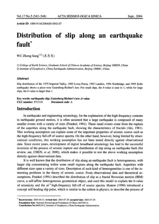
rupture. Figure 3 visualizes the distribution of slip for the Imperial Valley earthquake with exag-
gerations along the vertical axis and unequal scales along the strike and the dip directions. From
this schematic visualization it can be seen that the distribution of slip along an earthquake fault is
somehow similar to the topography of mountains. Therefore using the language of self-similarity
to describe the distribution of slip is an adequate choice. The result of this paper shows that

6. No.5 WUZhong-liang,et al: DISTRIBUTIONOF SLIPALONGANEARTHQUAKEFAULT 547
Gutenberg-Richter's power law dis-
tribution can be used to describe the
distribution of slip. But the differ-
ence is that not a single GR-relation,
but a piece-wise one, has to be used
to describe such a distribution.
In the synthesis of earthquake
strong ground motion which plays a
key role in the deterministic seismic
zonation, without sufficient knowl-
edge about the complexity of seismic
source process, generally some em-
pirical stochastic distributions are
used to describe the properties of
small events which determine the
high-frequency contents of ground
E
m
Figure 3 Distribution of slip for the Imperial Valley
earthquake(Dataare fromArchuleta,1984)
motion. Due to the limitation on observation in the past, such empirical stochastic distributions are
only from intuition or theoretical assumptions. The result obtained here provides the synthesis of
seismic strong ground motion with a useful model of source complexity.
If, as mentioned above, the crossover of the power laws does not come from the art-effects of
the subfault discretization in the inversion, then in physics it could be deduced that in the rupture
process of an earthquake, there are two types of events. One type is "large" events with b-value
larger 1. The reason for such a b-value is that these large events propagate along a single direction
and shows one-dimensional characteristics. Another type is "small" events with b-value near to 1.
These events are excited or triggered by the dynamics rupture process. The extension of these
small events along the time axis forms the weak aftershocks of the main shock.
The results obtained in this paper are only case studies for 5 earthquakes. More earthquakes
need to be investigated to explore the universality of the conclusions.
Acknowledgements Thanks are due to Prof. CHEN Yun-tai for guidance in the physics of
seismic source and digital seismology, and Prof. CHEN Yong for guidance in fractal geometry and
non-linear dynamics. Application of rank-ordei-ing analysis comes from the discussion with Prof.
D. Sornette and Prof. L. Knopoff.
References
Aki K. 1981. A probabilistic synthesisof precursory phenomena [A]. In: Simpson D W and Richards P G eds. Earthquake Prediction: An
International Review [C]. Washington,D. C.: AGU, 566~574.
Archuleta R J. 1984. A faulting model for the 1979 Imperial Valley earthquake [J]. J Geophys Res, 89:4 559~4 585.
CHEN Yun-tai, WU Zhong-liang,WANG Pei-de, et at. 2000. Digital Seismology [M]. Beijing: Seismological Press, 96~153 (in Chinese).
Frankel A. 1991. High-frequencyspectral falloff of earthquakes, fractal dimension of complex rupture, b value, and the scaling of strength
on faults [J]. J Geophys Res, 96:6 291~6 302.
Gutenberg B, Richter C E 1944. Frequency of earthquakes in California [J]. Bull Seism SocAmer, 34: 185~188.
Gutenberg B, Richter C E 1954. Seismicity of the Earth and Associated Phenomena (2nd ed) [M]. Princeton, NJ: Princeton Univ. Press,
1~310.
Heaton T H. 1990. Evidence for and implications of self-healing pulses of slip in earthquake rupture [J]. Phys Earth Planet Inter, 64:
1~20.
King G 1983. The accommodation of large strains in the upper lithosphere of the Earth and other solids by self-similarfault systems:The
geometrical origin of b-value [J]. PureAppl Geophys, 121: 761~815.
Mai P M, Beroza G C. 2000. Source scaling properties from finite-fanlt-rupturemodels [J]. Bull Seism SocAmer, 90: 604~615.

7. 548 ACTA SEISMOLOGICA S1NICA Vol. 17
Mai P M, Beroza G C. 2002. A spatial random field model to characterize complexity in earthquake slip [J].J Geophys Res, 107: Bll,
2308, doi: 10.1029/2001JB000588, ESE-10.
McGarr A, Fletcher J B. 2002. Mapping apparent stress and energy radiation over fault zones of major earthquakes [J]. Bull Seism Soc
Amer, 92:1 633-1 646.
Scholz C H. 1990. The Mechanics of Earthquakes and Faulting [M]. Cambridge: Cambridge Univ.Press, 160~221.
Sornette D, Knopoff L, Kagan Y Y, et al. 1996. Rank-ordering statistics of extreme events: Application to the distribution of large earth-
quakes [J].J Geophys Res, 101:13 883~13 893.
Turcotte D L. 1992.Fractals and Chaos in Geology and Geophysics [M]. Cambridge: Cambridge Univ. Press, 35~51.
Wald D J, Heaton T H, Hudnut K W. 1996. The slip history of the 1994 Northridge, California, earthquake determined from
strong-motion, teleseismic, GPS, and leveling data [J]. Bull Seism Soc Amer, 86: $49-$70.
Wald D J, Heaton T H. 1994. Spatial and temporal distribution of slip for the 1992 Landers, California, earthquake [J]. Bull Seism Soc
Amer, 84:668-691.
Wald D J, Helmberger D V, Heaton T H. 1991. Rupture model of the 1989 Loma Prieta earthquake from the inversion of strong-motion
and broadband teleseismic data [J].Bull Seism Soc Amer, 81:1 540~1 572.
Yoshida S, Koketsu K, Shibazaki B, et al. 1996. Joint inversion of near- and far-field waveforms and geodetic data for the rupture process
of the 1995 Kobe earthquake [J]. J Phys Earth, 44: 437-454.
Zipf G K. 1949.Human Behavior and the Principle of Least-Effort [M]. Reading, MA: Addison-Wesley.