Complexity

1. Complexity in Sequences of Solar Flares and Earthquakes
VLADIMIR G. KOSSOBOKOV,1
FABIO LEPRETI,2,3
and VINCENZO CARBONE
2,3
Abstract—In this paper the statistical properties of solar flares and earthquakes are compared by analyzing
the energy distributions, the time series of energies and interevent times, and, above all, the distributions of
interevent times per se. It is shown that the two phenomena have different statistics of scaling, and even the
same phenomenon, when observed in different periods or at different locations, is characterized by different
statistics that cannot be uniformly rescaled onto a single, universal curve. The results indicate apparent
complexity of impulsive energy release processes, which neither follow a common behaviour nor could be
attributed to a universal physical mechanism.
1. Introduction
Impulsive energy release events are observed in many natural systems. Solar flares
(e.g., ASCHWANDEN, 2004 and refs. therein) and earthquakes (GUTENBERG and RICHTER,
1954) are certainly among the most remarkable examples of such processes. Solar flares
are intense and sudden energy release events occurring in active regions of the solar
atmosphere. The source of flares is the energy stored in highly stressed magnetic field
configurations of the solar corona. During flares this energy is converted into accelerated
particles, electromagnetic radiation emission, plasma motions, and heat. The amount of
energy released in flares (reported to date) varies between roughly 1017
J and 1026
J.
Contrary to solar flares, whose origin and behavior we can currently observe in detail,
a coherent phenomenology on seismic events, which we evidence from their
consequences, is lacking. Apparently, earthquakes occur through frictional sliding along
the boundaries of highly stressed hierarchies of blocks of different sizes (from grains of
rock about 10-3
m to tectonic plates up to 107
m in linear dimension) that form the
lithosphere of the Earth (KEILIS-BOROK, 1990). The amount of energy released in
earthquakes varies from about 63 J in a detectable magnitude M = -2 event to more
1
International Institute of Earthquake Prediction Theory and Mathematical Geophysics, Russian Academy
of Sciences, 84/32 Profsoyuznaya, Moscow 117997, Russian Federation.
2
Dipartimento di Fisica, Universita` della Calabria, Ponte P. Bucci 31/C, I-87036 Rende, CS, Italy.
3
Consorzio Nazionale Interuniversitario per le Scienze Fisiche della Materia (CNISM), Unita` di Cosenza,
Ponte P. Bucci 31/C, I-87036 Rende, CS, Italy.
Pure appl. geophys. 165 (2008) 761–775 Ó Birkha¨user Verlag, Basel, 2008
0033–4553/08/030761–15
DOI 10.1007/s00024-008-0330-z
Pure and Applied Geophysics

2. than 1018
J in a magnitude M = 9 mega-earthquake (e.g., the recent 26 December 2004
Sumatra-Andaman, MW = 9.3 mega-thrust event is believed to release 4.3 9 1018
J).
Being recognized in the framework of plasma phenomena, the physics of solar flares
is rather well established (e.g., ASCHWANDEN, 2004 and refs. therein), while understanding
the physics of seismic events is more complicated (KEILIS-BOROK 1990; TURCOTTE, 1997;
DAVIES, 1999; GABRIELOV et al., 1999; KANAMORI and BRODSKY, 2001 and refs. therein)
regardless of the longer history of instrumental observations. Some fundamental integral
properties of seismic events are widely recognized in literature: (i) Following OMORI
(1894) many seismologists claim, with slight modifications, that n(t) *t-p
, where t is the
time span after the main shock, n(t) is the rate of occurrence of aftershocks at time t, and
p is a constant with a value of about 1; (ii) the number N(M) of earthquakes with
magnitude above a given threshold M in a given region behaves as logN(M) = a - bM,
where a and b are constants characterizing seismic activity and balance between
earthquakes of different size in the region (GUTENBERG and RICHTER, 1954); (iii)
earthquake epicenters follow fractal distribution in space (OKUBO and AKI, 1987;
TURCOTTE, 1997). Although the Omori law remains a controversy (UTSU et al., 1995),
there is growing evidence that distributed seismic activity obeys the unified scaling
law for earthquakes generalizing the Gutenberg-Richter relation as follows: logN(M,L) =
A – B (M – 5) + C log L, where N(M,L) is the expected annual number of earthquakes of
magnitude M within a seismic locus of liner size L (KOSSOBOKOV and MAZHKENOV, 1988;
KOSSOBOKOV and NEKRASOVA, 2005).
A statistical relation analogous to the Gutenberg-Richter law already has been found
for solar flare energy flux (see e.g., LIN et al., 1984; CROSBY et al., 1993). Moreover, the
interevent time Dt between solar flares has been shown to follow a power-law distribution
P(Dt) * Dt-a
(BOFFETTA et al., 1999) that suggests the Omori law analogue. Since the
two statistical relations seem to be roughly shared by both processes, the existence
of universality in the occurrence of these impulsive events was recently conjectured
(DE ARCANGELIS et al., 2006).
In this paper, the statistical properties of solar flares and earthquakes are compared by
analyzing the two sequences available from the Geostationary Operational Environmen-
tal Satellites (GOES) flare catalogue and the Southern California Seismic Network
(SCSN) earthquake catalogue. The temporal evolution of the two processes and the
probability distributions of event energies and interevent times are thoroughly
investigated. Unlike many studies based on probability density functions or histograms
(see e.g., BAK et al., 2002; CORRAL, 2003; DE ARCANGELIS et al., 2006), in order to reduce
the ambiguities and misinterpretations related to the choice of the binning we use the
cumulative probability distributions. This allows us to exploit the Kolmogorov-Smirnov
nonparametric criterion, the K-S test, when comparing different distributions either of
different phenomena, or in different periods of time, or at different locations. The paper is
organized as follows: The considered catalogues of solar flares and earthquakes are
briefly described in Section 2; the results of data analysis are presented in Section 3, and
discussed in Section 4.
762 V. G. Kossobokov et al. Pure appl. geophys.,

3. 2. Data
The catalogue of soft X-ray (SXR) solar flares used in this work was compiled from
observations of the Geostationary Operational Environmental Satellites (GOES) in the
wavelength band 1–8 A˚ . The catalogue consists of 62,212 events from September 1,
1975 to May 30, 2006 and covers the three most recent solar cycles. The catalogue and
the details about the event selection criteria can be found at the ftp site ftp://
ftp.ngdc.noaa.gov/. The GOES catalogue is the most complete data base on solar flare
bursts currently available. In order to classify the intensity of flares detected by GOES,
an index named GOES X-ray Class is used, which corresponds to the peak burst
intensity Ip measured in the wavelength band 1–8 A˚ . The classes are defined in
the following way: B class if Ip < 10-3
erg s-1
cm-2
, C class if 10-3
erg s-1
cm-2
< Ip < 10-2
erg s-1
cm-2
, M class if 10-2
erg s-1
cm-2
< Ip < 10-1
erg
s-1
cm-2
, and X class se Ip > 10-1
erg s-1
cm-2
. The class thus constitutes one of
the previous letters followed by a number which allows to identification of the value of
Ip, that is, for example a C4.6 class means that Ip = 4.6 9 10-3
erg s-1
cm-2
.
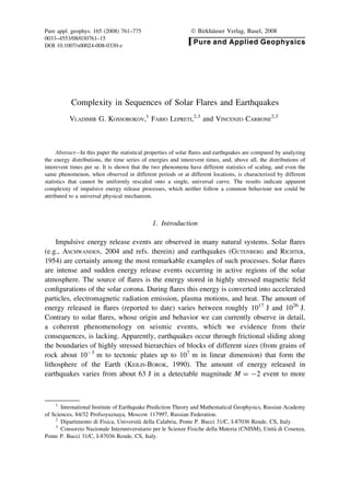
Beginning from January 1997, the integrated flux from event start to end is also
provided in the catalogue. Figure 1 shows the integrated flux as a function of the peak
burst intensity. A reasonably good proportionality between the two quantities is
observed, even if deviations from proportionality can be noted, especially for low and
intermediate energies. We can thus consider the X-ray class as a good proxy for energy
flux.
In the main part of our analysis, we considered the 32,076 flares of class C2 or larger.
This is because there is evidence for incompleteness of the catalogue for events of class
smaller than C2, as is explained in the next Section. In order to perform a separation
between the three cycles covered by the data set, we used the following simple criterion:
the boundary between two successive cycles corresponds to the longest interevent times
occurring between two C2+ flares. With this definition the three cycles cover the following
time intervals respectively: The first one (solar cycle 21) from September 1, 1975 to
September 8, 1986, the second one (solar cycle 22) from September 8, 1986 to August 22,
1996, and the third one (solar cycle 23) from August 22, 1996 until May 30, 2006.
The Southern California Earthquake Data Center (SCEDC) regularly compiles the
Southern California Seismographic Network (SCSN) catalogue of hypocentral informa-
tion. The catalogue started in 1932 and is being updated continuously. The data include
more than 450,000 local and regional events with epicenters mostly (i.e., more than 99%
of the total) between latitudes 32 and 37°N and longitudes between 114 and 122°W. For
information on catalogue completeness and data sources, see http://www.data.scec.org/
about/data_avail.html. In our study we consider catalogue completeness for the entire
region of Southern California, i.e., so-called magnitude completeness of the region. This
term should be distinguished from the so-called coverage completeness due to the
specifics of spatial distribution of a seismographic network. The magnitude completeness
is evidently different in relatively small areas at different locations, e.g., off-shore
Vol. 165, 2008 Complexity in Sequences of Solar Flares 763

4. Southern California or in the area of the Parkfield experiment. Moreover, in a small area
the catalogue availability might be too short in time for a decent evaluation of the
magnitude completeness. That is not the case of Southern California as a whole where the
SCSN catalogue is believed to be reasonably complete for seismic events greater than or
equal to M 3.0 since 1932, above M 1.8 since 1981, and for all magnitude events between
the time periods of January 1984 through the present. In the present study we use the
SCSN catalogue of earthquakes for the period 1986–2005, which contains 356,545
events. For the same reasons of completeness mentioned above for solar flares and
illustrated in the next Section, we consider the 87,688 earthquakes with magnitude M C 2
in the main part of the analysis. We also consider the aftershock series of the six strong
earthquakes in Southern California. The selection of the spatial and temporal span of the
aftershock series has been made by inspection of the epicenter maps in dynamics of
Figure 1
Integrated flux from event start to end for GOES flares (January 1997–May 2006) as a function of peak burst
intensity.
764 V. G. Kossobokov et al. Pure appl. geophys.,

5. seismic occurrences, so that the individually selected areas outline the evident clusters of
epicenters while the individually selected durations include the times of evident
activation of seismic activity next to the epicenter of the main shock. Such identification
of the individual clusters of seismic events is similar to identification of the flare
productive magnetic activity regions, which reference numbers reported in the GOES
catalogue of solar flares link flares occurring in the same cluster of activity.
3. Data Analysis and Results
3.1. Gutenberg-Richter Distributions
As was mentioned in the Introduction, both earthquake magnitudes and solar flare
energy fluxes are expected to be distributed in good agreement with the Gutenberg-Richter
law. Figure 2 shows the cumulative histograms of the peak intensity of the GOES flares
(upper plate) and of the magnitude of the SCSN earthquakes (lower plate). Along with the
total histograms, the ones for the three solar cycles and for each of the twenty years in the
SCSN catalogue are also given. (To facilitate inspection, straight lines with b = 1 are
plotted on both plates.)
As mentioned in the Introduction, the low energy cut-offs where the histograms start
deviating from the power-law Gutenberg-Richter behavior at low energies occur for flares
below GOES C2 class and for seismic events below magnitude 2.0. These deviations
indicate incompleteness of the catalogues in these regions and justify the thresholds
chosen to select the events used in the rest of our analysis. Some small bumps are clearly
visible in the flare distribution for the first cycle (for example for C2, M2 and X2 flares)
due to the poor resolution of event size in the initial years, as will be clearer from the
discussion of the next figure. It can also be seen that the earthquake distributions of
different years show consistent differences between them (e.g., the 1992 distribution) due
to the effect of the strongest events, as will be explained below.
3.2. Temporal Behavior
In order to have a first synoptic illustration of the two phenomena, we report in
Figure 3 the time series of the interevent times between successive events for both
catalogues, the time series of the peak GOES SXR intensities of solar flares and that of
the SCSN seismic event magnitudes.
The most prominent feature observable for solar flares is the effect of the activity cycle
resulting in an alternation of maximum periods, where the flaring activity is enhanced, and
minimum periods, where activity assumes a much more sporadic character. It can also be
seen that until roughly the end of 1980 the GOES classes (i.e., the peak intensities) were
given with the only one significant digit. This lack of resolution is at the origin of the small
bumps found in the cumulative peak SXR intensity histogram (previously shown) for the
Vol. 165, 2008 Complexity in Sequences of Solar Flares 765

6. Figure 2
Cumulative histograms of the GOES peak intensity of flares and of the SCSN magnitude of seismic events.
766 V. G. Kossobokov et al. Pure appl. geophys.,

7. solar cycle 21. For the seismic events, the time evolution is characterized by lengthy
periods of stable, slowly varying activity interrupted by the occurrence of strong activity
peaks corresponding to strong earthquakes with magnitude M > 6.
Another way to get an overall view of the two processes is to look at the frequencies
of the GOES class and SCSN magnitude respectively as functions of time. This is done
here by calculating the semi-annual number of flares in different GOES class intervals
and the annual number of earthquakes in different magnitude intervals (Fig. 4).
A number of evident features can be recognized from the solar flare plot. In the
central part of the cycles, around the solar maximum periods, intervals of roughly steady
activity are observed. In these intervals flares below C1 class are mostly missing., due to
the rise of the solar soft X-ray background associated with the maximum of magnetic
activity. It can also be seen that the time evolution of flaring activity is quite different in
the three cycles. For example, in the first cycle a quite steady and slow activity
enhancement is followed by a much faster decay, while in the second cycle two
successive enhancements and decreases can clearly be observed. The situation is even
more complex for the third cycle, where three or four distinct peaks of activity seem to be
present. Other remarkable features can be seen in the intervals between the cycles, which
should be characterized by low magnetic activity. Between the first and the second cycle
some clear activity bumps occur, while between the second and third cycle such
enhancements are absent. The earthquake magnitude-frequency versus time shown in the
lower panel of Figure 4 confirms once again that seismic events reported by SCSN
display a near stationary background activity interrupted by the occurrences of strong
earthquakes.
Figure 3
Time series of the interevent times between successive events for the GOES flares (upper-left) and for the SCSN
seismic events (upper-right). The solid lines represent moving averages over 50 events. Time series of the peak
GOES SXR intensity of flares (lower-left) and of the SCSN magnitude of seismic events (lower-right). Only
flares with GOES class above C2 and earthquakes with magnitude M C 2 were considered.
Vol. 165, 2008 Complexity in Sequences of Solar Flares 767

8. Figure 5 shows the accumulated number of events as a function of time both for flares
and earthquakes. The accumulated peak X-ray intensity for solar flares and the so-called
accumulated Benioff strain release for seismic events are also reported. The cumulative
Benioff strain release is an integral measure of fracturing defined by the sum of the square
root of the energy for consecutive events (see, e.g., VARNES, 1989; BUFE et al., 1994).
The time series of the accumulated number of flares shows a rather smooth evolution,
once again dominated by the solar cycle, with intervals of increase corresponding to the
activity maxima and nearly flat intervals corresponding to the solar minima. A similar
behavior is found in the accumulated peak X-ray intensity, although some differences in
timing can be observed, for example in the last part of the third cycle where the
Figure 4
Semi-annual number of flares in different GOES class intervals as a function of time (top panel) and annual
number of SCSN seismic events in different magnitude intervals as a function of time (bottom panel).
768 V. G. Kossobokov et al. Pure appl. geophys.,

9. accumulated number has become almost flat while the accumulated intensity is
continuously increasing. On the other hand, the two plots for seismic events both
display intervals of steady stationary increases interrupted by sudden jumps produced by
strong earthquakes and their aftershocks.
3.3. Inter-Event Time Distributions
We consider now the statistics of interevent times, that is, the time intervals
separating two consecutive events. In the upper panels of Figure 6 we report the
cumulative distribution of interevent times for GOES flares, both in semi-logarithmic and
bi-logarithmic scale. The cumulative distributions for the three different cycles are also
shown. In the lower panels of Figure 6 the interevent cumulative distributions of SCSN
seismic events are shown for the whole considered period and for each year separately.
Although the total flare interevent distributions and those for the three cycles show quite
similar power-law decay for times longer than 104
s, some differences can be seen even in
the power-law domain.
The differences between the distributions for seismic events are significant beyond any
doubt. It can be noted that the distributions of 1992 and 1999, which show the most evident
departure from the other ones, are dominated by the effect of the 1992 Landers and 1999
Hector Mine earthquakes and their sequences of associated fore- and aftershocks.
In order to study the differences of flaring and seismic activity between different
activity regions, we investigated the interevent time distributions of solar flares produced
in separate flare productive magnetic activity regions and those of the aftershocks
following the strongest earthquakes reported in the SCSN catalogue. The results are
plotted in Figure 7. It can be seen that different activity spots produce quite different
Figure 5
Accumulated number of events as a function of time for solar flares (lower-left) and earthquakes (lower-right).
The accumulated peak X-ray intensity for solar flares (upper-left) and the accumulated Benioff strain release for
seismic events (upper-right) are also shown.
Vol. 165, 2008 Complexity in Sequences of Solar Flares 769

10. interevent time distributions; the differences being stronger for seismic events than for
solar flares. Note that the 1992 Joshua Tree and Landers earthquakes, which occurred at
close locations and have shown up very similar distributions, are well separated in time.
To compare the statistical properties of interevent times of different impulsive energy
release processes, we report (Fig. 8) the cumulative interevent time distribution of all
GOES flares, GOES flares occurring in the same activity regions, all SCSN earthquakes,
and aftershocks of the Landers earthquake along with the cumulative interevent time
distribution of the unique long series of soft c-ray flashes on the neutron star 1806–20 (the
numbers are its celestial coordinates).
It is believed that flashes of energy radiated by a neutron star in the form of the soft
c-ray repeaters, SGRs, are probably generated by ‘‘starquakes’’ analogous to earthquakes
Figure 6
Cumulative distribution of interevent times for GOES flares (upper panels) and SCSN earthquakes (lower
panels), both in semi-logarithmic (left panels) and bi-logarithmic scale (right panels). The four distributions
shown for GOES flares refer to the whole period 1975–2006 (violet curve), to the first cycle 1975–1986 (blue
curve), to the second cycle 1986–1996 (green curve), and to the third cycle 1996–2006 (red curve) respectively.
The distributions of SCSN earthquakes are shown for the whole period 1986–2005 (black curve) and for each
year separately.
770 V. G. Kossobokov et al. Pure appl. geophys.,

11. (NORRIS et al., 1991; THOMPSON and DUNCAN, 1995). The source of a starquake is a fracture
in the neutron star crust, which may build up strain energy up to 1046
erg. The star 1806–20
is a dense ball about 20 km in diameter composed of neutrons. It weighs roughly as much
as the Sun, has the period of rotation about 7.5 s and the magnetic field of 1015
Gauss. Its
crust, made of a solid lattice of heavy nuclei with electrons flowing between, is 1 km thick.
The crust of a neutron star is loaded by magnetic forces as the field drifts through. These
forces cause fracturing of the crust and associated flashes of energy release. Starquakes are
of special interest due to the extreme energies released in a single event. The 111 flashes
on 1806–20 recorded during continuous observation from August 1978 to April 1985
follow power-law energy distribution and other earthquake-like statistics and behaviour
(KOSSOBOKOV et al., 2000).
The distributions presented in Figure 8 are very different. In order to check whether
they can be rescaled onto a single curve, we used the Kolmogoroff-Smirnoff two-sample
criterion. This test has the advantage of making no assumptions about the distribution of
Figure 7
Cumulative distributions of interevent times for GOES flares occurring in some flare productive active regions
(upper panels) and for aftershocks of some strong seismic events recorded in the SCSN catalogue (lower panels).
The distributions are shown both in semi-logarithmic scale (left panels) and bi-logarithmic scale (right panels).
The active zone numbers and main shock names are given in the legends.
Vol. 165, 2008 Complexity in Sequences of Solar Flares 771

12. Figure 8
Cumulative interevent time distributions of all GOES flares (blue curve), GOES flares occurring in the same
active regions (red curve), all SCSN earthquakes (green curve), and aftershocks of the Landers earthquake
(orange curve). The distributions are shown both in semi-logarithmic scale (upper panel) and in bi-logarithmic
scale (lower panel). The cumulative interevent time distribution of soft c-ray flashes of the SGR 1806–20,
attributed to starquakes produced by fractures in the neutron star crust, is also shown (light blue circles).
772 V. G. Kossobokov et al. Pure appl. geophys.,

13. data. Moreover, it is widely accepted to be one of the most useful and general
nonparametric methods for comparing two samples, as it is sensitive to differences
in both location and shape of the empirical cumulative distribution functions of the two
samples. The two sample Kolmogoroff-Smirnoff statistic kK-S is defined as
kK-S(D,n,m) = [nm/(n + m)]1/2
D, where D = max |P1,n(Dt) – P2,m(Dt)| is the maximum
value of the absolute difference between the cumulative distributions P1,n(Dt) and
P2,m(Dt) of the two samples, whose sizes are n and m, respectively. We calculated the
minimum values of kK-S, for all the couples of distributions over all rescaling fits of
the type P’(Dt) ¼ P(C Dta
), where C and a are fitting constants. These minimum values
are collected in Table 1 (above the diagonal) together with the corresponding
probabilities to reject the hypothesis of being drawn from the same distribution (under
the diagonal). The results indicate that only the associations of the ‘‘starquake’’
distribution, which is by far the sample of the smallest size, with the interevent time
distribution either of all flares, or activity spot flares, or the 1992 Landers earthquake
sequence cannot be rejected. For all the remaining cases, we can conclude with high
confidence that the distributions cannot be rescaled onto the same curve. For example, the
K-S test rejects a possibility that the interevent times between solar flares and those from
a single active region are drawn from the same distribution at the confidence level
starting with nine nines (i.e., 99.9999999%). In fact, the minimum of the maximal
difference D between the cumulative distributions reaches 3.15%, when C = 0.90 and
a ¼ 1.112, and due to the large sample sizes n and m implies kK-S(D, n, m) = 3.435 and
the above-mentioned level of confidence.
4. Discussion
Our comparison of the statistical properties of solar flares and seismic events shows
that, beside the expected global differences arising from the fact that solar flares are
related to the periodic solar activity cycle, the two phenomena are characterized by
different statistics of scaling. In fact, even the same phenomenon observed in different
Table 1
Results of the K-S test on the interevent time distributions shown in Figure 8. The sample sizes are reported on the
diagonal, the minimum values of kK-S over the rescaling fits described in the text are given above the diagonal
and the corresponding probabilities to reject the hypothesis of being drawn from the same distribution below the
diagonal
Flares Flares at spot SCSN Landers SGR1806–20
Flares 32076 3.435 8.648 2.071 0.636
Flares at spot 100.00% 18878 5.898 1.669 0.434
SCSN 100.00% 100.00% 87688 3.726 1.435
Landers 99.96% 99.26% 100.00% 10706 0.47
SGR1806–20 19.13% 0.92% 96.77% 2.24% 110
Vol. 165, 2008 Complexity in Sequences of Solar Flares 773

14. periods or locations (i.e., different solar active regions or aftershocks of different
earthquakes) can produce different probability distributions. Our analysis is mainly based
on the cumulative distributions of interevent times. Analyzing separately the interevent
time distributions of certain flare productive active regions, we have found that different
active regions give rise to substantially different statistics of the interevent times.
Remarkable differences are observed also in the interevent time statistics of aftershocks
of some strong (M > 6) seismic events present in the SCSN catalogue.
After constructing a data set with the interevent times between consecutive flares
occurring in the same active region, we have found that the interevent time distribution of
these flares displays a very different shape with respect to the distribution obtained taking
into account all solar flares. A clear power-law scaling ranging from 104
to 3 9 106
s is
found in the distribution for all flares, while the distribution for flares in individually
active regions has a more complex shape, which cannot be easily identified with a simple
law. The physical origin of this difference is an interesting question to be addressed in the
future. Similar complexity is observed in the interevent time statistics of the whole SCSN
seismic event catalogue as well as of the aftershock sequences of individually strong
earthquakes (e.g., the 1992 Landers event).
All these interevent time distributions have been compared to each other and also to
the unique distribution of the interevent time between starquakes produced by fracturing
of the neutron star crust. The main finding is that these distributions display a wide
variety of shapes and cannot be uniformly rescaled onto a single, universal curve by
natural two-parametric transforms of the interevent times. The small sample of
starquakes, which are of special interest due to the extreme energies released in a single
event and the uniqueness of the SGR1806–20 series, may appear similar to the others (the
similarity appears to be rejected just in the only case of the SCSN sample, the largest
among those considered) simply due to its size, which may not be enough for a confident
claim of specificity. Evidently, our results do not support the presence of universality and
the existence of a common physical mechanism at the origin of the energy release
phenomena considered. The statistical analogies between these phenomena should be
attributed rather to more general, integral properties of impulsive processes in critical,
nonlinear systems.
REFERENCES
ASCHWANDEN, M., Physics of the Solar Corona (Springer-Verlag, Berlin 2004).
BAK, P., CHRISTENSEN, K., DANON, L., and SCANLON, T. (2002), Unified scaling law for earthquakes, Phys. Rev.
Lett. 88, 178501.
BOFFETTA, G., CARBONE, V., GIULIANI, P., VELTRI, P., and VULPIANI, A. (1999), Power laws in solar flares: Self-
organized criticality or turbulence? Phys. Rev. Lett. 83, 4662–4665.
BUFE, C.G., NISHENKO, S.P., and VARNES, D.J. (1994), Seismicity trends and potential for large earthquakes in the
Alaska-Aleutian region, Pure Appl. Geophys. 142, 83–99.
CORRAL, A. (2003), Local distributions and rate fluctuations in a unified scaling law for earthquakes, Phys. Rev.
E 68, 035102.
774 V. G. Kossobokov et al. Pure appl. geophys.,

15. CROSBY, N.B., ASCHWANDEN, M.J., and DENNIS, B.R. (1993), Frequency distributions and correlations of solar
X-ray flare parameters, Solar Phys. 143, 275–299.
DAVIES, G.F., Dynamic Earth: Plates, Plumes and Mantle Convection, (Cambridge University Press, Cambridge
1999).
DE ARCANGELIS, L., GODANO, C., LIPPIELLO, E., and NICODEMI, M. (2006), Universality in solar flare and
earthquake occurrence, Phys. Rev. Lett. 96, 051102.
GABRIELOV, A., NEWMAN, W.I., and TURCOTTE, D.L. (1999), An exactly soluble hierarchical clustering model:
Inverse cascades, self-similarity, and scaling, Phys. Rev. E 60, 5293–5300.
GUTENBERG, B., and RICHTER, C.F., Seismicity of the Earth, 2nd ed. (Princeton University Press, Princeton,
N.J. 1954).
KANAMORI, H. and BRODSKY, E.H. (2001), The Physics of Earthquakes, Physics Today, June 2001, 34–40.
KEILIS-BOROK, V.I. (1990), The lithosphere of the Earth as a nonlinear system with implications for earthquake
prediction, Rev. Geophys. 28 (1), 19–34.
KOSSOBOKOV, V.G. and MAZHKENOV, S.A., Spatial characteristics of similarity for earthquake sequences:
Fractality of seismicity, Lecture Notes of the Workshop on Global Geophysical Informatics with Applications
to Research in Earthquake Prediction and Reduction of Seismic Risk (15 Nov.–16 Dec., 1988), 15 pp., (ICTP,
Trieste 1988).
KOSSOBOKOV, V.G., KEILIS-BOROK, V.I., and CHENG, B. (2000), Similarities of multiple fracturing on a neutron
star and on the Earth, Phys. Rev. E 61, 3529–3533.
KOSSOBOKOV, V.G. and NEKRASOVA, A.K. (2005), Temporal variations in the parameters of the Unified Scaling
Law for Earthquakes in the eastern part of Honshu Island (Japan), Doklady Earth Sciences 405, 1352–1356.
LIN, R.P., SCHWARTZ, R.A., KANE, S.R., PELLING, R.M., and HURLEY, K.C. (1984), Solar hard X-ray microflares,
Astrophys. J. 283, 421–425.
NORRIS, J.P., HERZ, P., WOOD, K.S., and KOUVELIOTOU, C. (1991), On the nature of soft gamma repeaters,
Astrophys. J. 366, 240–252.
OKUBO, P.G., and AKI, K. (1987), Fractal geometry in the San Andreas Fault system, J. Geophys. Res. 92 (B1),
345–356.
OMORI, F. (1894), On the after-shocks of earthquakes, J. Coll. Sci. Imp. Univ. Tokyo 7, 111–200.
THOMPSON, C., and DUNCAN, R. C. (1995), The soft gamma repeaters as very strongly magnetized neutron stars -
I. Radiative mechanism for outbursts, Mon. Not. R. Astr. Soc. 275, 255–300.
TURCOTTE, D.L., Fractals and Chaos in Geology and Geophysics, 2nd edition, (Cambridge University Press,
Cambridge 1997).
UTSU, T., OGATA, Y., and MATSU’URA, R.S. (1995), The centenary of the Omori formula for a decay law of
aftershock activity, J. Phys. Earth 43, 1–33.
VARNES, D.J. (1989), Predicting earthquakes by analyzing accelerating precursory seismic activity, Pure Appl.
Geophys. 130, 661–686.
(Received December 22, 2006, revised March 30, 2007, accepted March 30, 2007)
Published Online First: April 2, 2008
To access this journal online:
www.birkhauser.ch/pageoph
Vol. 165, 2008 Complexity in Sequences of Solar Flares 775