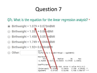
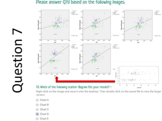
Download as PDF, PPTX


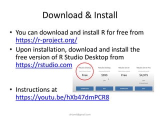


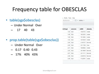
![Compute mBMI=weight/(height/100)^2
• sga$mBMI <-
(sga$weight/(sga$height)^2)
• View(sga)
• mean(sga$mBMI)
– [1] 24.49576
• sd(sga$mBMI)
– [1] 4.767109](https://image.slidesharecdn.com/introtorrstudio-200618030547/85/Introduction-to-Data-Analysis-With-R-and-R-Studio-17-320.jpg)
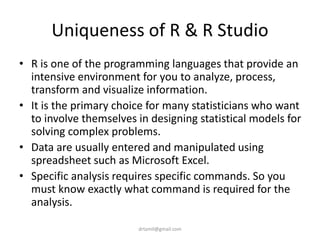
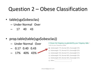
![Question 1 – BMI
• mean(sga$mBMI)
– [1] 24.49576
• sd(sga$mBMI)
– [1] 4.767109](https://image.slidesharecdn.com/introtorrstudio-200618030547/85/Introduction-to-Data-Analysis-With-R-and-R-Studio-18-320.jpg)
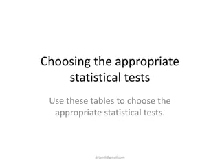
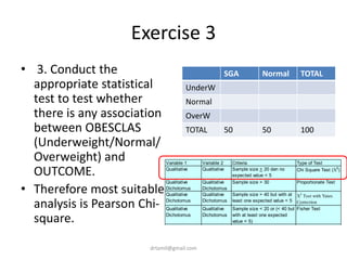
![Recode mBMI into OBESCLAS
• sga$obesclas<-""
• sga$obesclas[sga$mBMI<20] <- 1
• sga$obesclas[sga$mBMI>=20 &
sga$mBMI<25] <- 2
• sga$obesclas[sga$mBMI>=25] <- 3
• table(sga$obesclas)
• sga$obesclas <-
factor(sga$obesclas, levels =
c(1,2,3),labels = c('Under',
'Normal', 'Over'))
• table(sga$obesclas)
drtamil@gmail.com](https://image.slidesharecdn.com/introtorrstudio-200618030547/85/Introduction-to-Data-Analysis-With-R-and-R-Studio-20-320.jpg)
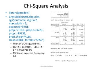
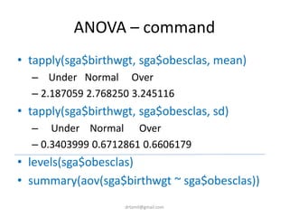
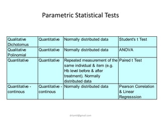
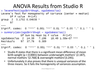
![ANOVA – Results
• > levels(sga$obesclas)
• [1] "Under" "Normal" "Over"
• > summary(aov(sga$birthwgt ~ sga$obesclas))
• Df Sum Sq Mean Sq F value Pr(>F)
• sga$obesclas 2 14.39 7.196 18.49 1.58e-07 ***
• Residuals 97 37.76 0.389
• ---
• Signif. codes: 0 ‘***’ 0.001 ‘**’ 0.01 ‘*’ 0.05 ‘.’ 0.1 ‘ ’ 1
drtamil@gmail.com](https://image.slidesharecdn.com/introtorrstudio-200618030547/85/Introduction-to-Data-Analysis-With-R-and-R-Studio-37-320.jpg)
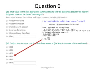
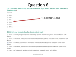
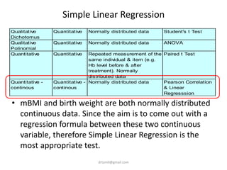
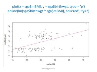
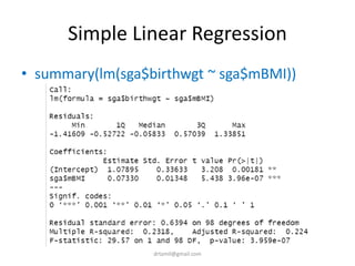
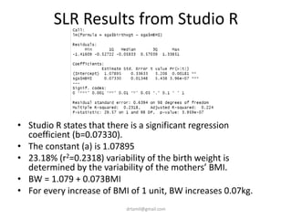
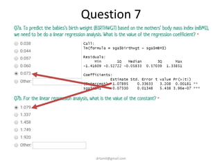


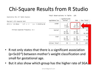
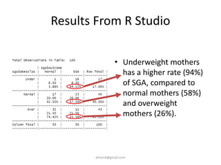
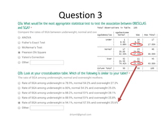
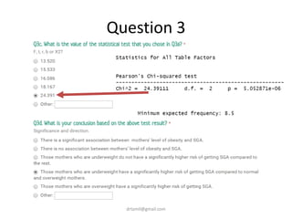
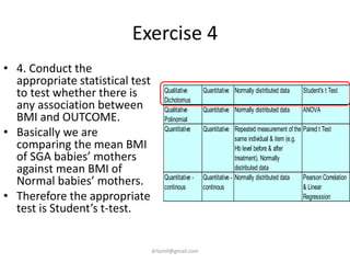
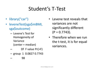
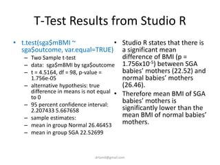
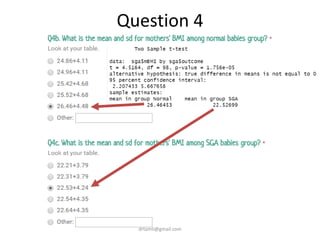
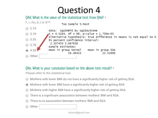
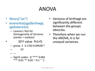
- A study analyzed factors that can cause babies to be small for gestational age (SGA), including mothers' body mass index (BMI). - The document discusses computing BMI from height and weight data, classifying BMI into underweight, normal, and overweight categories, and performing statistical tests to analyze associations between these factors and birthweight and SGA outcomes. - Statistical tests discussed include chi-square tests, t-tests, ANOVA, and linear regression to identify relationships between maternal BMI, weight classification, and baby's birthweight and risk of SGA.