EFFECT SIZE
More to life than statistical significance
Reporting effect size
STATISTICAL SIGNIFICANCE
 Turns out a lot of researchers do not know
what precisely p < .05 actually means
 Cohen (1994) Article: The earth is round
(p<.05)
 What it means: "Given that H0 is true, what
is the probability of these (or more extreme)
data?”
 Trouble is most people want to know "Given
these data, what is the probability that H0 is
true?"
ALWAYS A DIFFERENCE
 With most analyses we commonly define the null
hypothesis as ‘no relationship’ between our
predictor and outcome(i.e. the ‘nil’ hypothesis)
 With sample data, differences between groups
always exist (at some level of precision),
correlations are always non-zero.
 Obtaining statistical significance can be seen as
just a matter of sample size
 Furthermore, the importance and magnitude of an
effect are not accurately reflected because of the
role of sample size in probability value attained
WHAT SHOULD WE BE DOING?
 We want to make sure we have looked hard
enough for the difference – power analysis
 Figure out how big the thing we are looking for is –
effect size
CALCULATING EFFECT SIZE
 Though different statistical tests have different
effect sizes developed for them, the general
principle is the same
 Effect size refers to the magnitude of the impact of
some variable on another
TYPES OF EFFECT SIZE
 Two basic classes of effect size
 Focused on standardized mean differences for
group comparisons
 Allows comparison across samples and variables with
differing variance
 Equivalent to z scores
 Note sometimes no need to standardize (units of the
scale have inherent meaning)
 Variance-accounted-for
 Amount explained versus the total
 d family vs. r family
 With group comparisons we will also talk about
case-level effect sizes
COHEN’S D (HEDGE’S G)
 Cohen was one of the pioneers in advocating effect
size over statistical significance
 Defined d for the one-sample case
X
d
s



COHEN’S D
 Note the similarity to a z-score- we’re talking about
a standardized difference
 The mean difference itself is a measure of effect
size, however taking into account the variability, we
obtain a standardized measure for comparison of
studies across samples such that e.g. a d =.20 in
this study means the same as that reported in
another study
COHEN’S D
 Now compare to the one-sample t-statistic
 So
 This shows how the test statistic (and its observed p-
value) is in part determined by the effect size, but is
confounded with sample size
 This means small effects may be statistically significant in
many studies (esp. social sciences)
X
X
t
s
N



t
t d N and d
N
 
COHEN’S D – DIFFERENCES BETWEEN
MEANS
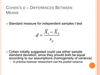
 Standard measure for independent samples t test
 Cohen initially suggested could use either sample
standard deviation, since they should both be equal
according to our assumptions (homogeneity of variance)
 In practice however researchers use the pooled variance
1 2
p
X X
d
s


EXAMPLE
Average number of times graduate
psych students curse in the presence
of others out of total frustration over
the course of a day
Currently taking a statistics course vs.
not
Data:
2
2
13 7.5 30
11 5.0 30
s
n
X s n
X s n
  
  
EXAMPLE
 Find the pooled variance and sd
 Equal groups so just average the two variances such
that and sp
2 = 6.25
13 11
.8
6.25
d

 
COHEN’S D – DIFFERENCES BETWEEN
MEANS
 Relationship to t
 Relationship to rpb
1 2
1 1
d t
n n
 
1 2
2
1 2
2 1 1
1
pb
pb
n n
d r
n n
r
  
 
 
  
 
  
 
2
(1/ )
d
r
d pq


P and q are the proportions of the total each group makes up.
If equal groups p=.5, q=.5 and the denominator is d2 + 4 as you will see
in some texts
GLASS’S Δ
 For studies with control groups, we’ll use the control
group standard deviation in our formula
 This does not assume equal variances
1 2
control
X X
d
s


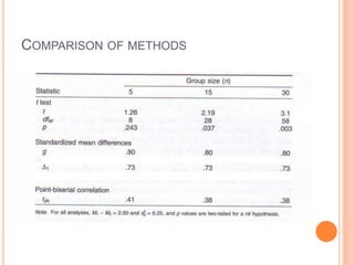
COMPARISON OF METHODS
DEPENDENT SAMPLES
 One option would be to simply do nothing different
than we would in the independent samples case,
and treat the two sets of scores as independent
 Problem:
 Homogeneity of variance assumption may not be
tenable
 They aren’t independent
DEPENDENT SAMPLES
 Another option is to obtain a metric with
regard to the actual difference scores on
which the test is run
 A d statistic for a dependent mean contrast
is called a standardized mean change (gain)
 There are two general standardizers:
 A standard deviation in the metric of the
 1. difference scores (D)
 2. original scores
DEPENDENT SAMPLES
 Difference scores
 Mean difference score divided by the standard
deviation of the difference scores
D
D
d
s

DEPENDENT SAMPLES
 The standard deviation of the difference scores, unlike the previous
solution, takes into account the correlated nature of the data
 Var1 + Var2 – 2covar
 Problems remain however
 A standardized mean change in the metric of the difference scores
can be much different than the metric of the original scores
 Variability of difference scores might be markedly different for change
scores compared to original units
 Interpretation may not be straightforward
12
2(1 )
D p
D D
d
s s r
 

DEPENDENT SAMPLES
 Another option is to use standardizer in the metric
of the original scores, which is directly comparable
with a standardized mean difference from an
independent-samples design
 In pre-post types of situations where one would not
expect homogeneity of variance, treat the pretest
group of scores as you would the control for Glass’s
Δ
p
D
d
s

DEPENDENT SAMPLES
• Base it on substantive theoretical
interest
• If the emphasis is really on
change, i.e. the design is
intrinsically repeated measures,
one might choose the option of
standardized mean change
• In other situations we might retain
the standardizer in the original
metric, such that the d will have
the same meaning as elsewhere
Which to use?
CHARACTERIZING EFFECT SIZE
 Cohen emphasized that the interpretation of effects
requires the researcher to consider things narrowly
in terms of the specific area of inquiry
 Evaluation of effect sizes inherently requires a
personal value judgment regarding the practical or
clinical importance of the effects
HOW BIG?
 Cohen (e.g. 1969, 1988) offers some rules of thumb
 Fairly widespread convention now (unfortunately)
 Looked at social science literature and suggested some
ways to carve results into small, medium, and large
effects
 Cohen’s d values (Lipsey 1990 ranges in parentheses)
 0.2 small (<.32)
 0.5 medium (.33-.55)
 0.8 large (.56-1.2)
 Be wary of “mindlessly invoking” these criteria
 The worst thing that we could do is subsitute d = .20 for
p = .05, as it would be a practice just as lazy and fraught
with potential for abuse as the decades of poor practices
we are currently trying to overcome
SMALL, MEDIUM, LARGE?
 Cohen (1969)
 ‘small’
 real, but difficult to detect
 difference between the heights of 15 year old and 16 year old
girls in the US
 Some gender differences on aspects of Weschler Adult
Intelligence scale
 ‘medium’
 ‘large enough to be visible to the naked eye’
 difference between the heights of 14 & 18 year old girls
 ‘large’
 ‘grossly perceptible and therefore large’
 difference between the heights of 13 & 18 year old girls
 IQ differences between PhDs and college freshman
ASSOCIATION
 A measure of association describes the
amount of the covariation between the
independent and dependent variables
 It is expressed in an unsquared
standardized metric or its squared value—
the former is usually a correlation*, the latter
a variance-accounted-for effect size
 A squared multiple correlation (R2)
calculated in ANOVA is called the correlation
ratio or estimated eta-squared (2)
ANOTHER MEASURE OF EFFECT SIZE
 The point-biserial correlation, rpb, is the
Pearson correlation between membership in
one of two groups and a continuous
outcome variable
 As mentioned rpb has a direct relationship to
t and d
 When squared it is a special case of eta-
squared in ANOVA
 An one-way ANOVA for a two-group factor:
eta-squared = R2 from a regression approach
= r2
pb
ETA-SQUARED
 A measure of the degree to which variability
among observations can be attributed to
conditions
 Example: 2 = .50
 50% of the variability seen in the scores is due to the
independent variable.
2 2
treat
pb
total
SS
R
SS
  
ETA-SQUARED
 Relationship to t in the two group setting
2
2
2
t
t df
 

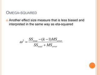
OMEGA-SQUARED
 Another effect size measure that is less biased and
interpreted in the same way as eta-squared
2 ( 1)
treat error
total error
SS k MS
SS MS

 


PARTIAL ETA-SQUARED
 A measure of the degree to which variability among
observations can be attributed to conditions controlling
for the subjects’ effect that’s unaccounted for by the
model (individual differences/error)
 Rules of thumb for small medium large: .01, .06, .14
 Note that in one-way design SPSS labels this as PES but
is actually eta-squared, as there is only one factor and no
others to partial out
2
partialη treat
treat error
SS
SS SS


COHEN’S F
 Cohen has a d type of measuere for Anova called f
 Cohen's f is interpreted as how many standard
deviation units the means are from the grand mean,
on average, or, if all the values were standardized, f
is the standard deviation of those standardized
means
2
..
( )
e
X X
k
f
MS



RELATION TO PES
Using Partial Eta-Squared
1
PES
f
PES


GUIDELINES
 As eta-squared values are basically r2 values
the feel for what is large, medium and small is
similar and depends on many contextual factors
 Small eta-squared and partial eta-square
values might not get the point across (i.e. look
big enough to worry about)
 Might transform to Cohen’s f or use so as to continue
to speak of standardized mean differences
 His suggestions for f are: .10,.25,.40 which translate
to .01,.06, and .14 for eta-squared values
 That is something researchers could overcome if
they understood more about effect sizes
OTHER EFFECT SIZE MEASURES
 Measures of association for non-continuous
data
 Contingency coefficient
 Phi
 Cramer’s Phi
 d-family
 Odds Ratios
 Agreement
 Kappa
 Case level effect sizes
CONTINGENCY COEFFICIENT
 An approximation of the correlation between the
two variables (e.g. 0 to 1)
 Problem- can’t ever reach 1 and its max value is
dependent on the dimensions of the contingency
table
2
2
C
N




PHI
 Used in 2 X 2 tables as a correlation (0 to 1)
 Problem- gets weird with more complex tables
2
N

 
CRAMER’S PHI
 Again think of it as a measure of association from 0
(weak) to 1 (strong), that is phi for 2X2 tables but
also works for more complex ones.
 k is the lesser of the number of rows or columns
2
( 1)
c
N k

 

ODDS RATIOS
 Especially good for 2X2 tables
 Take a ratio of two outcomes
 Although neither gets the majority, we could
say which they were more likely to vote for
respectively
 Odds Clinton among Dems= 564/636 = .887
 Odds McCain among Reps= 450/550 = .818
 .887/.818 (the odds ratio) means they’d be
1.08 times as likely to vote Clinton among
democrats than McCain among republicans
 However, the 95% CI for the odds ratio is:
 .92 to 1.28
 This suggests it would not be wise to predict
either has a better chance at nomination at this
point.
 Numbers coming from
 Feb 1-3
 Gallup Poll daily tracking. Three-day rolling
average. N=approx. 1,200 Democrats and
Democratic-leaning voters nationwide.
 Gallup Poll daily tracking. Three-day rolling
average. N=approx. 1,000 Republican and
Republican-leaning voters nationwide.
Yes No Total
Clinton 564 636 1200
McCain 450 550 1000
KAPPA
 Measure of agreement (from Cohen)
 Though two folks (or groups of
people) might agree, they might also
have a predisposition to respond in a
certain way anyway
 Kappa takes this into consideration to
determine how much agreement
there would be after incorporating
what we would expect by chance
 O and E refer to the observed and
expected frequencies on the diagonal
of the table of Judge 1 vs Judge 2






D
D
D
E
N
E
O
K
Judge 1 Totals
Judge 2 1 2 3
1 10 (5.5) 2 0 12
2 1 5 (3.67) 2 8
3 0 1 3 (.88) 4
11 8 5 24
%
57
95
.
13
95
.
7


K
Judgements by clinical psycholgists
on the severity of suicide attempts by clients.
At first glance one might think (10+5+3)/24 =
75% agreement between the two.
However this does not take into account
chance agreement.
CASE-LEVEL EFFECT SIZES
 Indexes such as Cohen’s d and eta2 estimate effect
size at the group or variable level only
 However, it is often of interest to estimate
differences at the case level
 Case-level indexes of group distinctiveness are
proportions of scores from one group versus
another that fall above or below a reference point
 Reference points can be relative (e.g., a certain
number of standard deviations above or below the
mean in the combined frequency distribution) or
more absolute (e.g., the cutting score on an
admissions test)
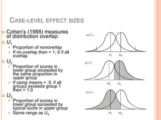
CASE-LEVEL EFFECT SIZES
 Cohen’s (1988) measures
of distribution overlap:
 U1
 Proportion of nonoverlap
 If no overlap then = 1, 0 if all
overlap
 U2
 Proportion of scores in
lower group exceeded by
the same proportion in
upper group
 If same means = .5, if all
group2 exceeds group 1
then = 1.0
 U3
 Proportion of scores in
lower group exceeded by
typical score in upper group
 Same range as U2
OTHER CASE-LEVEL EFFECT SIZES
 Tail ratios (Feingold, 1995):
Relative proportion of scores
from two different groups that
fall in the upper extreme (i.e.,
either the left or right tail) of the
combined frequency
distribution
 “Extreme” is usually defined
relatively in terms of the
number of standard deviations
away from the grand mean
 Tail ratio > 1.0 indicates one
group has relatively more
extreme scores
 Here, tail ratio = p2/p1:
OTHER CASE-LEVEL EFFECT SIZES
 Common language effect size (McGraw &
Wong, 1992) is the predicted probability that
a random score from the upper group
exceeds a random score from the lower
group
 Find area to the right of that value
 Range .5 – 1.0
1 2
2 2
1 2
0 ( )
CL
X X
z
s s
 


CONFIDENCE INTERVALS FOR EFFECT
SIZE
Effect size statistics such as Hedge’s g
and η2 have complex distributions
Traditional methods of interval
estimation rely on approximate
standard errors assuming large
sample sizes
General form for d
( )
cv d
d t s

CONFIDENCE INTERVALS FOR EFFECT
SIZE
 Standard errors
2
1 2
2
2 1 2
2
/
2( )
2( )
2(1 )
/
2( 1)
w
d N
d g
df n n
N
n n n
Dependent Samples
d r
d g
n n
 

  

 

PROBLEM
 However, CIs formulated in this manner are only
approximate, and are based on the central (t)
distribution centered on zero
 The true (exact) CI depends on a noncentral
distribution and additional parameter
 Noncentrality parameter
 What the alternative hype distribution is centered on
(further from zero, less belief in the null)
 d is a function of this parameter, such that if ncp = 0
(i.e. is centered on the null hype value), then d = 0
(i.e. no effect)
1 2
1 2
pop
n n
d ncp
n n


CONFIDENCE INTERVALS FOR EFFECT
SIZE
Similar situation for r and eta2 effect
size measures
Gist: we’ll need a computer program to
help us find the correct noncentrality
parameters to use in calculating exact
confidence intervals for effect sizes
Statistica has such functionality built
into its menu system while others
allow for such intervals to be
programmed (even SPSS scripts are
available (Smithson))
LIMITATIONS OF EFFECT SIZE
MEASURES
 Standardized mean differences:
 Heterogeneity of within-conditions variances across
studies can limit their usefulness—the unstandardized
contrast may be better in this case
 Measures of association:
 Correlations can be affected by sample variances and
whether the samples are independent or not, the design is
balanced or not, or the factors are fixed or not
 Also affected by artifacts such as missing observations,
range restriction, categorization of continuous variables,
and measurement error (see Hunter & Schmidt, 1994, for
various corrections)
 Variance-accounted-for indexes can make some effects
look smaller than they really are in terms of their
substantive significance
LIMITATIONS OF EFFECT SIZE
MEASURES
 How to fool yourself with effect size estimation:
 1. Examine effect size only at the group level
 2. Apply generic definitions of effect size magnitude without
first looking to the literature in your area
 3. Believe that an effect size judged as “large” according to
generic definitions must be an important result and that a
“small” effect is unimportant (see Prentice & Miller, 1992)
 4. Ignore the question of how theoretical or practical
significance should be gauged in your research area
 5. Estimate effect size only for statistically significant results
LIMITATIONS OF EFFECT SIZE
MEASURES
 6. Believe that finding large effects somehow lessens the need for
replication
 7. Forget that effect sizes are subject to sampling error
 8. Forget that effect sizes for fixed factors are specific to the
particular levels selected for study
 9. Forget that standardized effect sizes encapsulate other quantities
such as the unstandardized effect size, error variance, and
experimental design
 10. As a journal editor or reviewer, substitute effect size magnitude
for statistical significance as a criterion for whether a work is
published
 11. Think that effect size = cause size
RECOMMENDATIONS
 First recall APA task force suggestions
 Report effect sizes
 Report confidence intervals
 Use graphics
RECOMMENDATIONS
 Report and interpret effect sizes in the context of
those seen in previous research rather than rules of
thumb
 Report and interpret confidence intervals (for effect
sizes too) also within the context of prior research
 In other words don’t be overly concerned with whether a CI
for a mean difference doesn’t contain zero but where it
matches up with previous CIs
 Summarize prior and current research with the
display of CIs in graphical form (e.g. w/ Tryon’s
reduction)
 Report effect sizes even for nonsig results
RESOURCES
 Kline, R. (2004) Beyond significance
testing.
 Much of the material for this lecture came from
this
 Rosnow, R & Rosenthal, R. (2003). Effect
Sizes for Experimenting Psychologists.
Canadian JEP 57(3).
 Thompson, B. (2002). What future
Quantitative Social Science Research could
look like: Confidence intervals for effect
sizes. Educational Researcher.

effectsize.ppt

  • 1.
    EFFECT SIZE More tolife than statistical significance Reporting effect size
  • 2.
    STATISTICAL SIGNIFICANCE  Turnsout a lot of researchers do not know what precisely p < .05 actually means  Cohen (1994) Article: The earth is round (p<.05)  What it means: "Given that H0 is true, what is the probability of these (or more extreme) data?”  Trouble is most people want to know "Given these data, what is the probability that H0 is true?"
  • 3.
    ALWAYS A DIFFERENCE With most analyses we commonly define the null hypothesis as ‘no relationship’ between our predictor and outcome(i.e. the ‘nil’ hypothesis)  With sample data, differences between groups always exist (at some level of precision), correlations are always non-zero.  Obtaining statistical significance can be seen as just a matter of sample size  Furthermore, the importance and magnitude of an effect are not accurately reflected because of the role of sample size in probability value attained
  • 4.
    WHAT SHOULD WEBE DOING?  We want to make sure we have looked hard enough for the difference – power analysis  Figure out how big the thing we are looking for is – effect size
  • 5.
    CALCULATING EFFECT SIZE Though different statistical tests have different effect sizes developed for them, the general principle is the same  Effect size refers to the magnitude of the impact of some variable on another
  • 6.
    TYPES OF EFFECTSIZE  Two basic classes of effect size  Focused on standardized mean differences for group comparisons  Allows comparison across samples and variables with differing variance  Equivalent to z scores  Note sometimes no need to standardize (units of the scale have inherent meaning)  Variance-accounted-for  Amount explained versus the total  d family vs. r family  With group comparisons we will also talk about case-level effect sizes
  • 7.
    COHEN’S D (HEDGE’SG)  Cohen was one of the pioneers in advocating effect size over statistical significance  Defined d for the one-sample case X d s   
  • 8.
    COHEN’S D  Notethe similarity to a z-score- we’re talking about a standardized difference  The mean difference itself is a measure of effect size, however taking into account the variability, we obtain a standardized measure for comparison of studies across samples such that e.g. a d =.20 in this study means the same as that reported in another study
  • 9.
    COHEN’S D  Nowcompare to the one-sample t-statistic  So  This shows how the test statistic (and its observed p- value) is in part determined by the effect size, but is confounded with sample size  This means small effects may be statistically significant in many studies (esp. social sciences) X X t s N    t t d N and d N  
  • 10.
    COHEN’S D –DIFFERENCES BETWEEN MEANS  Standard measure for independent samples t test  Cohen initially suggested could use either sample standard deviation, since they should both be equal according to our assumptions (homogeneity of variance)  In practice however researchers use the pooled variance 1 2 p X X d s  
  • 11.
    EXAMPLE Average number oftimes graduate psych students curse in the presence of others out of total frustration over the course of a day Currently taking a statistics course vs. not Data: 2 2 13 7.5 30 11 5.0 30 s n X s n X s n      
  • 12.
    EXAMPLE  Find thepooled variance and sd  Equal groups so just average the two variances such that and sp 2 = 6.25 13 11 .8 6.25 d   
  • 13.
    COHEN’S D –DIFFERENCES BETWEEN MEANS  Relationship to t  Relationship to rpb 1 2 1 1 d t n n   1 2 2 1 2 2 1 1 1 pb pb n n d r n n r                  2 (1/ ) d r d pq   P and q are the proportions of the total each group makes up. If equal groups p=.5, q=.5 and the denominator is d2 + 4 as you will see in some texts
  • 14.
    GLASS’S Δ  Forstudies with control groups, we’ll use the control group standard deviation in our formula  This does not assume equal variances 1 2 control X X d s  
  • 15.
  • 16.
    DEPENDENT SAMPLES  Oneoption would be to simply do nothing different than we would in the independent samples case, and treat the two sets of scores as independent  Problem:  Homogeneity of variance assumption may not be tenable  They aren’t independent
  • 17.
    DEPENDENT SAMPLES  Anotheroption is to obtain a metric with regard to the actual difference scores on which the test is run  A d statistic for a dependent mean contrast is called a standardized mean change (gain)  There are two general standardizers:  A standard deviation in the metric of the  1. difference scores (D)  2. original scores
  • 18.
    DEPENDENT SAMPLES  Differencescores  Mean difference score divided by the standard deviation of the difference scores D D d s 
  • 19.
    DEPENDENT SAMPLES  Thestandard deviation of the difference scores, unlike the previous solution, takes into account the correlated nature of the data  Var1 + Var2 – 2covar  Problems remain however  A standardized mean change in the metric of the difference scores can be much different than the metric of the original scores  Variability of difference scores might be markedly different for change scores compared to original units  Interpretation may not be straightforward 12 2(1 ) D p D D d s s r   
  • 20.
    DEPENDENT SAMPLES  Anotheroption is to use standardizer in the metric of the original scores, which is directly comparable with a standardized mean difference from an independent-samples design  In pre-post types of situations where one would not expect homogeneity of variance, treat the pretest group of scores as you would the control for Glass’s Δ p D d s 
  • 21.
    DEPENDENT SAMPLES • Baseit on substantive theoretical interest • If the emphasis is really on change, i.e. the design is intrinsically repeated measures, one might choose the option of standardized mean change • In other situations we might retain the standardizer in the original metric, such that the d will have the same meaning as elsewhere Which to use?
  • 22.
    CHARACTERIZING EFFECT SIZE Cohen emphasized that the interpretation of effects requires the researcher to consider things narrowly in terms of the specific area of inquiry  Evaluation of effect sizes inherently requires a personal value judgment regarding the practical or clinical importance of the effects
  • 23.
    HOW BIG?  Cohen(e.g. 1969, 1988) offers some rules of thumb  Fairly widespread convention now (unfortunately)  Looked at social science literature and suggested some ways to carve results into small, medium, and large effects  Cohen’s d values (Lipsey 1990 ranges in parentheses)  0.2 small (<.32)  0.5 medium (.33-.55)  0.8 large (.56-1.2)  Be wary of “mindlessly invoking” these criteria  The worst thing that we could do is subsitute d = .20 for p = .05, as it would be a practice just as lazy and fraught with potential for abuse as the decades of poor practices we are currently trying to overcome
  • 24.
    SMALL, MEDIUM, LARGE? Cohen (1969)  ‘small’  real, but difficult to detect  difference between the heights of 15 year old and 16 year old girls in the US  Some gender differences on aspects of Weschler Adult Intelligence scale  ‘medium’  ‘large enough to be visible to the naked eye’  difference between the heights of 14 & 18 year old girls  ‘large’  ‘grossly perceptible and therefore large’  difference between the heights of 13 & 18 year old girls  IQ differences between PhDs and college freshman
  • 25.
    ASSOCIATION  A measureof association describes the amount of the covariation between the independent and dependent variables  It is expressed in an unsquared standardized metric or its squared value— the former is usually a correlation*, the latter a variance-accounted-for effect size  A squared multiple correlation (R2) calculated in ANOVA is called the correlation ratio or estimated eta-squared (2)
  • 26.
    ANOTHER MEASURE OFEFFECT SIZE  The point-biserial correlation, rpb, is the Pearson correlation between membership in one of two groups and a continuous outcome variable  As mentioned rpb has a direct relationship to t and d  When squared it is a special case of eta- squared in ANOVA  An one-way ANOVA for a two-group factor: eta-squared = R2 from a regression approach = r2 pb
  • 27.
    ETA-SQUARED  A measureof the degree to which variability among observations can be attributed to conditions  Example: 2 = .50  50% of the variability seen in the scores is due to the independent variable. 2 2 treat pb total SS R SS   
  • 28.
    ETA-SQUARED  Relationship tot in the two group setting 2 2 2 t t df   
  • 29.
    OMEGA-SQUARED  Another effectsize measure that is less biased and interpreted in the same way as eta-squared 2 ( 1) treat error total error SS k MS SS MS     
  • 30.
    PARTIAL ETA-SQUARED  Ameasure of the degree to which variability among observations can be attributed to conditions controlling for the subjects’ effect that’s unaccounted for by the model (individual differences/error)  Rules of thumb for small medium large: .01, .06, .14  Note that in one-way design SPSS labels this as PES but is actually eta-squared, as there is only one factor and no others to partial out 2 partialη treat treat error SS SS SS  
  • 31.
    COHEN’S F  Cohenhas a d type of measuere for Anova called f  Cohen's f is interpreted as how many standard deviation units the means are from the grand mean, on average, or, if all the values were standardized, f is the standard deviation of those standardized means 2 .. ( ) e X X k f MS   
  • 32.
    RELATION TO PES UsingPartial Eta-Squared 1 PES f PES  
  • 33.
    GUIDELINES  As eta-squaredvalues are basically r2 values the feel for what is large, medium and small is similar and depends on many contextual factors  Small eta-squared and partial eta-square values might not get the point across (i.e. look big enough to worry about)  Might transform to Cohen’s f or use so as to continue to speak of standardized mean differences  His suggestions for f are: .10,.25,.40 which translate to .01,.06, and .14 for eta-squared values  That is something researchers could overcome if they understood more about effect sizes
  • 34.
    OTHER EFFECT SIZEMEASURES  Measures of association for non-continuous data  Contingency coefficient  Phi  Cramer’s Phi  d-family  Odds Ratios  Agreement  Kappa  Case level effect sizes
  • 35.
    CONTINGENCY COEFFICIENT  Anapproximation of the correlation between the two variables (e.g. 0 to 1)  Problem- can’t ever reach 1 and its max value is dependent on the dimensions of the contingency table 2 2 C N    
  • 36.
    PHI  Used in2 X 2 tables as a correlation (0 to 1)  Problem- gets weird with more complex tables 2 N   
  • 37.
    CRAMER’S PHI  Againthink of it as a measure of association from 0 (weak) to 1 (strong), that is phi for 2X2 tables but also works for more complex ones.  k is the lesser of the number of rows or columns 2 ( 1) c N k    
  • 38.
    ODDS RATIOS  Especiallygood for 2X2 tables  Take a ratio of two outcomes  Although neither gets the majority, we could say which they were more likely to vote for respectively  Odds Clinton among Dems= 564/636 = .887  Odds McCain among Reps= 450/550 = .818  .887/.818 (the odds ratio) means they’d be 1.08 times as likely to vote Clinton among democrats than McCain among republicans  However, the 95% CI for the odds ratio is:  .92 to 1.28  This suggests it would not be wise to predict either has a better chance at nomination at this point.  Numbers coming from  Feb 1-3  Gallup Poll daily tracking. Three-day rolling average. N=approx. 1,200 Democrats and Democratic-leaning voters nationwide.  Gallup Poll daily tracking. Three-day rolling average. N=approx. 1,000 Republican and Republican-leaning voters nationwide. Yes No Total Clinton 564 636 1200 McCain 450 550 1000
  • 39.
    KAPPA  Measure ofagreement (from Cohen)  Though two folks (or groups of people) might agree, they might also have a predisposition to respond in a certain way anyway  Kappa takes this into consideration to determine how much agreement there would be after incorporating what we would expect by chance  O and E refer to the observed and expected frequencies on the diagonal of the table of Judge 1 vs Judge 2       D D D E N E O K Judge 1 Totals Judge 2 1 2 3 1 10 (5.5) 2 0 12 2 1 5 (3.67) 2 8 3 0 1 3 (.88) 4 11 8 5 24 % 57 95 . 13 95 . 7   K Judgements by clinical psycholgists on the severity of suicide attempts by clients. At first glance one might think (10+5+3)/24 = 75% agreement between the two. However this does not take into account chance agreement.
  • 40.
    CASE-LEVEL EFFECT SIZES Indexes such as Cohen’s d and eta2 estimate effect size at the group or variable level only  However, it is often of interest to estimate differences at the case level  Case-level indexes of group distinctiveness are proportions of scores from one group versus another that fall above or below a reference point  Reference points can be relative (e.g., a certain number of standard deviations above or below the mean in the combined frequency distribution) or more absolute (e.g., the cutting score on an admissions test)
  • 41.
    CASE-LEVEL EFFECT SIZES Cohen’s (1988) measures of distribution overlap:  U1  Proportion of nonoverlap  If no overlap then = 1, 0 if all overlap  U2  Proportion of scores in lower group exceeded by the same proportion in upper group  If same means = .5, if all group2 exceeds group 1 then = 1.0  U3  Proportion of scores in lower group exceeded by typical score in upper group  Same range as U2
  • 42.
    OTHER CASE-LEVEL EFFECTSIZES  Tail ratios (Feingold, 1995): Relative proportion of scores from two different groups that fall in the upper extreme (i.e., either the left or right tail) of the combined frequency distribution  “Extreme” is usually defined relatively in terms of the number of standard deviations away from the grand mean  Tail ratio > 1.0 indicates one group has relatively more extreme scores  Here, tail ratio = p2/p1:
  • 43.
    OTHER CASE-LEVEL EFFECTSIZES  Common language effect size (McGraw & Wong, 1992) is the predicted probability that a random score from the upper group exceeds a random score from the lower group  Find area to the right of that value  Range .5 – 1.0 1 2 2 2 1 2 0 ( ) CL X X z s s    
  • 44.
    CONFIDENCE INTERVALS FOREFFECT SIZE Effect size statistics such as Hedge’s g and η2 have complex distributions Traditional methods of interval estimation rely on approximate standard errors assuming large sample sizes General form for d ( ) cv d d t s 
  • 45.
    CONFIDENCE INTERVALS FOREFFECT SIZE  Standard errors 2 1 2 2 2 1 2 2 / 2( ) 2( ) 2(1 ) / 2( 1) w d N d g df n n N n n n Dependent Samples d r d g n n          
  • 46.
    PROBLEM  However, CIsformulated in this manner are only approximate, and are based on the central (t) distribution centered on zero  The true (exact) CI depends on a noncentral distribution and additional parameter  Noncentrality parameter  What the alternative hype distribution is centered on (further from zero, less belief in the null)  d is a function of this parameter, such that if ncp = 0 (i.e. is centered on the null hype value), then d = 0 (i.e. no effect) 1 2 1 2 pop n n d ncp n n  
  • 47.
    CONFIDENCE INTERVALS FOREFFECT SIZE Similar situation for r and eta2 effect size measures Gist: we’ll need a computer program to help us find the correct noncentrality parameters to use in calculating exact confidence intervals for effect sizes Statistica has such functionality built into its menu system while others allow for such intervals to be programmed (even SPSS scripts are available (Smithson))
  • 48.
    LIMITATIONS OF EFFECTSIZE MEASURES  Standardized mean differences:  Heterogeneity of within-conditions variances across studies can limit their usefulness—the unstandardized contrast may be better in this case  Measures of association:  Correlations can be affected by sample variances and whether the samples are independent or not, the design is balanced or not, or the factors are fixed or not  Also affected by artifacts such as missing observations, range restriction, categorization of continuous variables, and measurement error (see Hunter & Schmidt, 1994, for various corrections)  Variance-accounted-for indexes can make some effects look smaller than they really are in terms of their substantive significance
  • 49.
    LIMITATIONS OF EFFECTSIZE MEASURES  How to fool yourself with effect size estimation:  1. Examine effect size only at the group level  2. Apply generic definitions of effect size magnitude without first looking to the literature in your area  3. Believe that an effect size judged as “large” according to generic definitions must be an important result and that a “small” effect is unimportant (see Prentice & Miller, 1992)  4. Ignore the question of how theoretical or practical significance should be gauged in your research area  5. Estimate effect size only for statistically significant results
  • 50.
    LIMITATIONS OF EFFECTSIZE MEASURES  6. Believe that finding large effects somehow lessens the need for replication  7. Forget that effect sizes are subject to sampling error  8. Forget that effect sizes for fixed factors are specific to the particular levels selected for study  9. Forget that standardized effect sizes encapsulate other quantities such as the unstandardized effect size, error variance, and experimental design  10. As a journal editor or reviewer, substitute effect size magnitude for statistical significance as a criterion for whether a work is published  11. Think that effect size = cause size
  • 51.
    RECOMMENDATIONS  First recallAPA task force suggestions  Report effect sizes  Report confidence intervals  Use graphics
  • 52.
    RECOMMENDATIONS  Report andinterpret effect sizes in the context of those seen in previous research rather than rules of thumb  Report and interpret confidence intervals (for effect sizes too) also within the context of prior research  In other words don’t be overly concerned with whether a CI for a mean difference doesn’t contain zero but where it matches up with previous CIs  Summarize prior and current research with the display of CIs in graphical form (e.g. w/ Tryon’s reduction)  Report effect sizes even for nonsig results
  • 53.
    RESOURCES  Kline, R.(2004) Beyond significance testing.  Much of the material for this lecture came from this  Rosnow, R & Rosenthal, R. (2003). Effect Sizes for Experimenting Psychologists. Canadian JEP 57(3).  Thompson, B. (2002). What future Quantitative Social Science Research could look like: Confidence intervals for effect sizes. Educational Researcher.