This document discusses sampling of continuous-time signals to create discrete-time signals. It explains that for perfect reconstruction, the sampling frequency must be greater than twice the maximum frequency of the original continuous-time signal, as specified by the Nyquist rate. Common sampling methods include impulse train sampling and zero-order hold sampling. Zero-order hold sampling approximates the signal between samples by holding the value constant, and is often sufficient to reconstruct the original continuous-time signal.

1. Lecture 10: Sampling Discrete-Time Systems
4 Sampling & Discrete-time systems (2 lectures):
Sampling theorem, discrete Fourier transform
Specific objectives for today:
• Sampling of a continuous-time signal
• Reconstruction of the signals from its samples
• Sampling theorem & Nyquist rate
• Reconstruction of a signal, using zero-order holds

2. Lecture 10: Resources
Core reading
SaS, O&W, C7
Background reading
MIT Lectures 9 & 13
In these two lectures, we’re going to develop the DT
Fourier transform as a sampled version of the CT
Fourier transform.
Note that this is opposite to time-domain convolution
where we developed CT convolution as the limiting
case of DT convolution

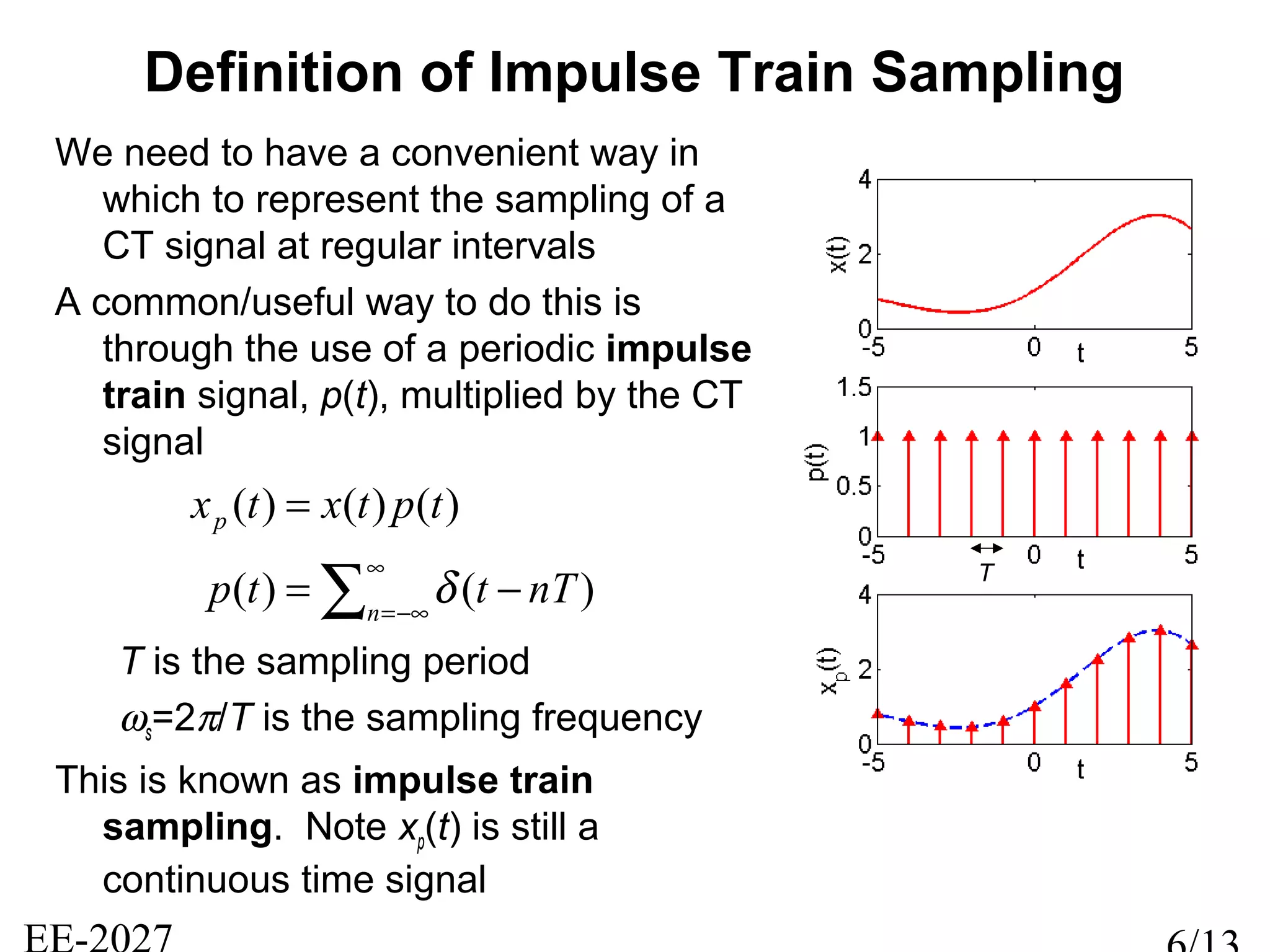
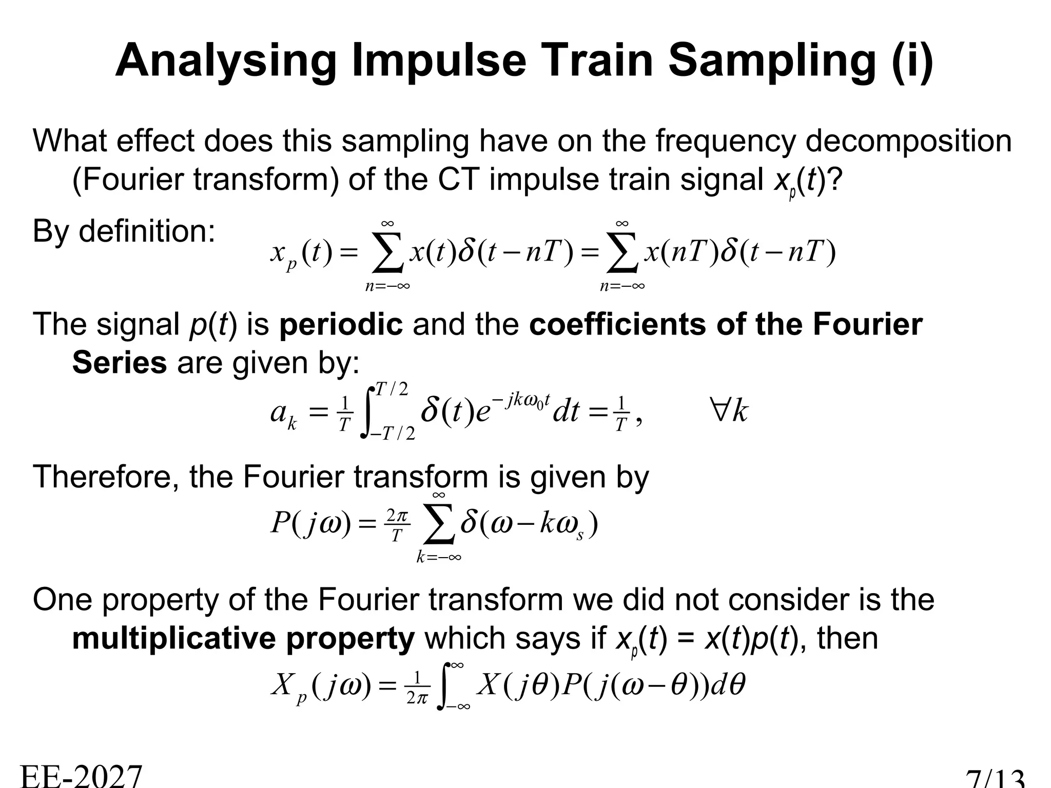
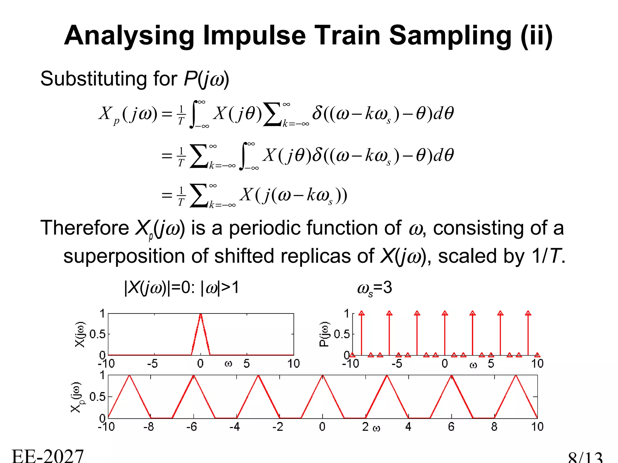
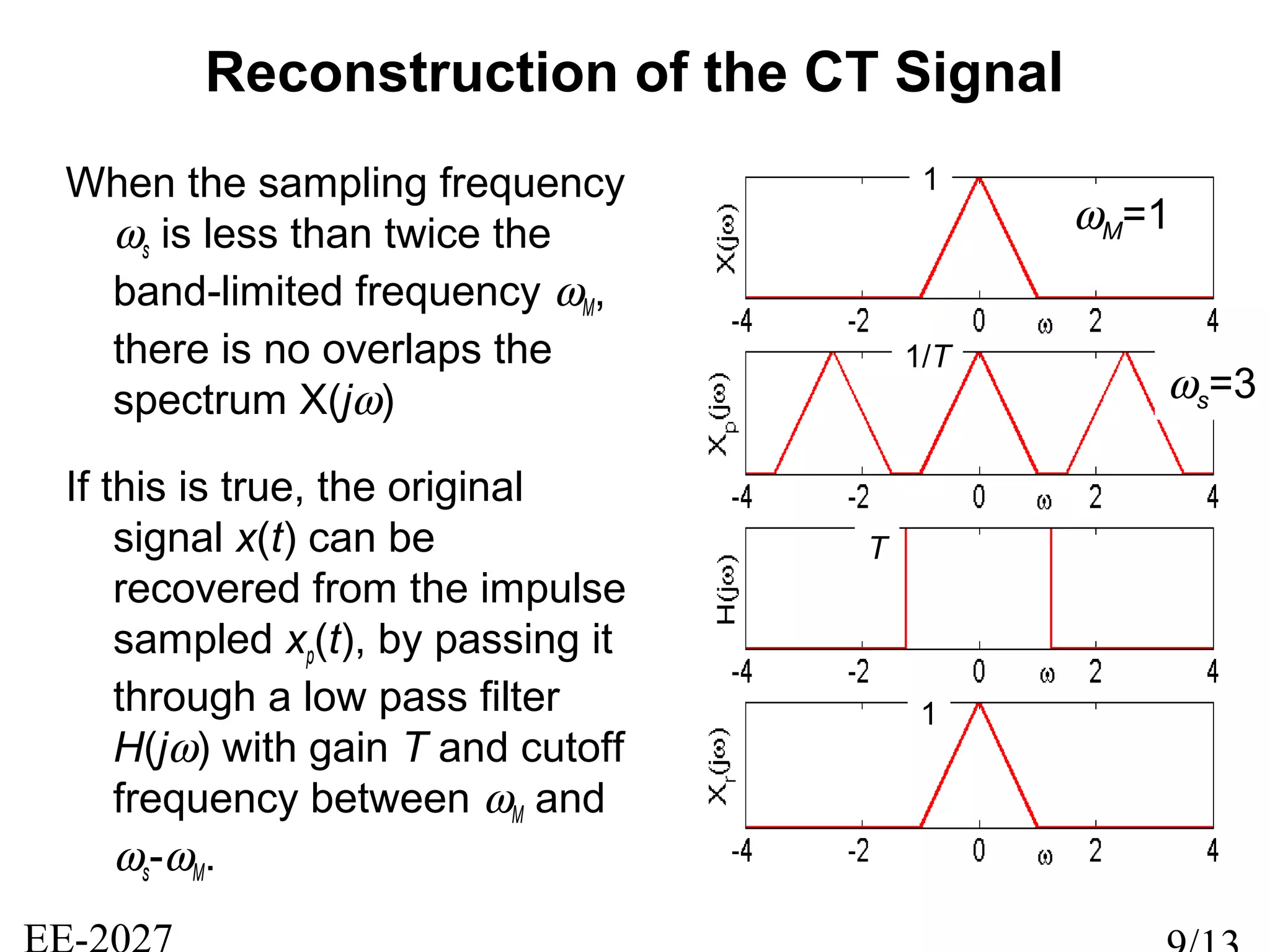
3. Sampling is the transformation of a continuous signal
into a discrete signal
Widely applied in digital analysis systems
1. Sample the continuous time signal
2. Design and process discrete time signal
3. Convert back to continuous time
What is Discrete Time Sampling?
x(t),
x[n]
t=nT
Discrete
Time sampler
Discrete
time system
Signal
reconstruction
x(t) x[n] y[n] y(t)
T is the sampling
period

4. Why is Sampling Important?
For many systems (e.g. Matlab, …) designing and
processing discrete-time systems is more efficient and
more general compared to performing continuous-time
system design.
How does Simulink perform continuous-time system
simulation?
The signals are sampled and the systems are approximately
integrated in discrete time
Mainly due to the dramatic development of digital technology
resulting in inexpensive, lightweight, programmable and
reproducible discrete-time systems. Widely used for
communication

5. Sampling a Continuous-Time Signal
Clearly for a finite sample period T, it is not possible to represent
every uncountable, infinite-dimensional continuous-time signal
with a countable, infinite-dimensional discrete-time signal.
In general, an infinite number of CT signals can generate a DT
signal.
However, if the signal is band (frequency) limited, and the
samples are sufficiently close, it is possible to uniquely
reconstruct the original CT signal from the sampled signal
x1(t),
x2(t),
x3(t),
x[n]
t=nT

6. Definition of Impulse Train Sampling
We need to have a convenient way in
which to represent the sampling of a
CT signal at regular intervals
A common/useful way to do this is
through the use of a periodic impulse
train signal, p(t), multiplied by the CT
signal
T is the sampling period
ωs=2π/T is the sampling frequency
This is known as impulse train
sampling. Note xp(t) is still a
continuous time signal
∑
∞
−∞=
−=
=
n
p
nTttp
tptxtx
)()(
)()()(
δ T

7. Analysing Impulse Train Sampling (i)
What effect does this sampling have on the frequency decomposition
(Fourier transform) of the CT impulse train signal xp(t)?
By definition:
The signal p(t) is periodic and the coefficients of the Fourier
Series are given by:
Therefore, the Fourier transform is given by
One property of the Fourier transform we did not consider is the
multiplicative property which says if xp(t) = x(t)p(t), then
∑∑
∞
−∞=
∞
−∞=
−=−=
nn
p nTtnTxnTttxtx )()()()()( δδ
∫
∞
∞−
−= θθωθω π djPjXjX p ))(()()( 2
1
∑
∞
−∞=
−=
k
sT kjP )()( 2
ωωδω π
kdteta T
T
T
tjk
Tk ∀== ∫−
−
,)( 1
2/
2/
1 0ω
δ

8. Analysing Impulse Train Sampling (ii)
Substituting for P(jω)
Therefore Xp(jω) is a periodic function of ω, consisting of a
superposition of shifted replicas of X(jω), scaled by 1/T.
∑
∑ ∫
∫ ∑
∞
−∞=
∞
−∞=
∞
∞−
∞
∞−
∞
−∞=
−=
−−=
−−=
k sT
k sT
k sTp
kjX
dkjX
dkjXjX
))((
))(()(
))(()()(
1
1
1
ωω
θθωωδθ
θθωωδθω
|X(jω)|=0: |ω|>1 ωs=3

9. Reconstruction of the CT Signal
When the sampling frequency
ωs is less than twice the
band-limited frequency ωM,
there is no overlaps the
spectrum X(jω)
If this is true, the original
signal x(t) can be
recovered from the impulse
sampled xp(t), by passing it
through a low pass filter
H(jω) with gain T and cutoff
frequency between ωM and
ωs-ωM.
1
1/T
T
1
ωM=1
ωs=3

10. Sampling Theorem
Let x(t) be a band (frequency)-limited signal
X(jω) = 0 for |ω|>ωM.
Then x(t) is uniquely determined by its samples {x(nT)}
when the sampling frequency satisfies:
where ωs=2π/T.
2ωM is known as the Nyquist rate, as it represents the
largest frequency that can be reproduced with the sample
time
The result makes sense because a frequency-limited signal
has a limited amount of information that can be fully
captured with the sampled sequence {x(nT)}
Ms ωω 2>
X(jω)
ωM ω
ωs
-ωM

11. Zero Order Hold Sampling
A zero order hold is a common method
for bridging CT-DT signals
A zero order hold samples the current
signal and holds that value until the
next sample
In most systems, it is difficult to
generate and transmit narrow, large-
amplitude pulses (impulse train
sampling) xp(t)
We can often use a variety of
filtering/interpolation techniques to
reconstruct the original time-domain
signal, however often the zero-order
hold signal x0(t) is sufficiently
accurate
xp(t)
x0(t)
x(t)
t
t
t

12. Lecture 10: Summary
The sample time for converting a continuous time signal into
a sampled, discrete time signal is determined by the
Nyquist rate, amongst other things.
The signal must satisfy the relationship:
If the signal is to be preserved exactly. Information in
frequencies higher than this will be lost when the signal is
sampled.
A continuous time signal is often sampled and communicated
using a zero order hold
Often this is enough to be considered as the re-constructed
continuous time signal, but sometimes approximate
methods for re-constructing the signal are used
Ms ωω 2>

13. Lecture 10: Exercises
Theory
SaS, O&W, 7.1-7.4, 7.7