SlideShare a Scribd company logo
1 of 13
Download to read offline
CS/EE 5590 / ENG 401 Special Topics
(Class Ids: 17804, 17815, 17803)
Lec 02
Entropy and Lossless Coding I
Zhu Li
Z. Li Multimedia Communciation, 2016 Spring p.1
Outline
 Lecture 01 ReCap
 Info Theory on Entropy
 Lossless Entropy Coding
Z. Li Multimedia Communciation, 2016 Spring p.2
Video Compression in Summary
Z. Li Multimedia Communciation, 2016 Spring p.3
Video Coding Standards: Rate-Distortion Performance
 Pre-HEVC
Z. Li Multimedia Communciation, 2016 Spring p.4
PSS over managed IP networks
 Managed mobile core IP networks
Z. Li Multimedia Communciation, 2016 Spring p.5
MPEG DASH – OTT
 HTTP Adaptive Streaming of Video
Z. Li Multimedia Communciation, 2016 Spring p.6
Outline
 Lecture 01 ReCap
 Info Theory on Entropy
 Self Info of an event
 Entropy of the source
 Relative Entropy
 Mutual Info
 Entropy Coding
Thanks for SFU’s Prof. Jie Liang’s slides!
Z. Li Multimedia Communciation, 2016 Spring p.7
Entropy and its Application
Entropy coding: the last part of a compression system
Losslessly represent symbols
Key idea:
 Assign short codes for common symbols
 Assign long codes for rare symbols
Question:
 How to evaluate a compression method?
o Need to know the lower bound we can achieve.
o  Entropy
Entropy
coding
QuantizationTransform
Encoder
0100100101111
Z. Li Multimedia Communciation, 2016 Spring p.8
Claude Shannon: 1916-2001
 A distant relative of Thomas Edison
 1932: Went to University of Michigan.
 1937: Master thesis at MIT became the foundation of
digital circuit design:
o “The most important, and also the most famous,
master's thesis of the century“
 1940: PhD, MIT
 1940-1956: Bell Lab (back to MIT after that)
 1948: The birth of Information Theory
o A mathematical theory of communication, Bell System
Technical Journal.
Z. Li Multimedia Communciation, 2016 Spring p.9
Axiom Definition of Information
Information is a measure of uncertainty or surprise
 Axiom 1:
 Information of an event is a function of its probability:
i(A) = f (P(A)). What’s the expression of f()?
 Axiom 2:
 Rare events have high information content
 Water found on Mars!!!
 Common events have low information content
 It’s raining in Vancouver.
Information should be a decreasing function of the probability:
Still numerous choices of f().
 Axiom 3:
 Information of two independent events = sum of individual information:
If P(AB)=P(A)P(B)  i(AB) = i(A) + i(B).
 Only the logarithmic function satisfies these conditions.
Z. Li Multimedia Communciation, 2016 Spring p.10
Self-information
)(log
)(
1
log)( xp
xp
xi bb 
• Shannon’s Definition [1948]:
• X: discrete random variable with alphabet {A1, A2, …, AN}
• Probability mass function: p(x) = Pr{ X = x}
• Self-information of an event X = x:
If b = 2, unit of information is bit
Self information indicates the number of bits
needed to represent an event.
1
P(x)
)(log xPb
0
Z. Li Multimedia Communciation, 2016 Spring p.11
 Recall: the mean of a function g(X):
Entropy is the expected self-information of the r.v. X:
 The entropy represents the minimal number of bits needed to
losslessly represent one output of the source.
Entropy of a Random Variable

x xp
xpXH
)(
1
log)()(
)g()())(()( xxpXgE xp 
 )(log
)(
1
log )()( XpE
Xp
EH xpxp 






Also write as H (p): function of the distribution of X, not the value of X.
Z. Li Multimedia Communciation, 2016 Spring p.12
Example
P(X=0) = 1/2
P(X=1) = 1/4
P(X=2) = 1/8
P(X=3) = 1/8
Find the entropy of X.
Solution:
1
( ) ( )log
( )
1 1 1 1 1 2 3 3 7
log 2 log 4 log8 log8 bits/sample.
2 4 8 8 2 4 8 8 4
x
H X p x
p x

        

Z. Li Multimedia Communciation, 2016 Spring p.13
Example
A binary source: only two possible outputs: 0, 1
 Source output example: 000101000101110101……
 p(X=0) = p, p(X=1)= 1 – p.
Entropy of X:
 H(p) = p (-log2(p) ) + (1-p) (-log2(1-p))
 H = 0 when p = 0 or p =1
oFixed output, no information
 H is largest when p = 1/2
oHighest uncertainty
oH = 1 bit in this case
Properties:
 H ≥ 0
 H concave (proved later) 0 0.1 0.2 0.3 0.4 0.5 0.6 0.7 0.8 0.9 1
0
0.2
0.4
0.6
0.8
1
p
Entropy
Equal prob maximize entropy
Z. Li Multimedia Communciation, 2016 Spring p.14
Joint entropy
1 1 2 2( , , )n np X i X i X i  
• We can get better understanding of the source S by looking at a block
of output X1X2…Xn:
• The joint probability of a block of output:
 Joint entropy
1 2
1 2
1 1 2 2
1 1 2 2
( , , )
1
( , , )log
( , , )n
n
n n
i i i n n
H X X X
p X i X i X i
p X i X i X i

  
  
 

 

 Joint entropy is the number of bits required to represent the
sequence X1X2…Xn:
 This is the lower bound for entropy coding.
 ),...(log 1 nXXpE
Z. Li Multimedia Communciation, 2016 Spring p.15
Conditional Entropy
1 ( )
( | ) log log
( | ) ( , )
p y
i x y
p x y p x y
 
• Conditional Self-Information of an event X = x, given that
event Y = y has occurred:
 ( , )
( | ) ( ) ( | ) ( ) ( | )log( ( | ))
( | ) ( )log( ( | )) ( , )log( ( | ))
log( ( | )
x x y
x y x y
p x y
H Y X p x H Y X x p x p y x p y x
p y x p x p y x p x y p y x
E p y x
   
   
 
  
 
 Conditional Entropy H(Y | X): Average cond. self-info.
Remaining uncertainty about Y given the knowledge of X.
Note: p(x | y), p(x, y) and p(y) are three different distributions:
p1(x | y), p2(x, y) and p3(y).
Z. Li Multimedia Communciation, 2016 Spring p.16
Conditional Entropy
Example: for the following joint distribution p(x, y), find H(Y |
X).
1 2 3 4
1 1/8 1/16 1/32 1/32
2 1/16 1/8 1/32 1/32
3 1/16 1/16 1/16 1/16
4 1/4 0 0 0
Y
X
( | ) ( ) ( | )log( ( | )) ( , )log( ( | ))
x y x y
H Y X p x p y x p y x p x y p y x     
Need to find conditional prob p(y | x)
( , )
( | )
( )
p x y
p y x
p x
 Need to find marginal prob p(x) first (sum columns).
P(X): [ ½, ¼, 1/8, 1/8 ] >> H(X) = 7/4 bits
P(Y): [ ¼ , ¼, ¼, ¼ ] >> H(Y) = 2 bits
H(X|Y) = ∑ = ( | = )
= ¼ H(1/2 ¼ 1/8 1/8 )
+ 1/4H(1/4, ½, 1/8 ,1/8)
+ 1/4H(1/4 ¼ ¼ ¼ ) +
1/4H(1 0 0 0)
= 11/8 bits
Z. Li Multimedia Communciation, 2016 Spring p.17
Chain Rule
H(X, Y) = H(X) + H(Y|X) = H(Y) + H(X|Y)
Proof:
H(X) H(Y)
H(X | Y) H(Y | X)
Total area: H(X, Y)
 








x
x yx y
x y
x y
XYHXHXYHxpxp
xypyxpxpyxp
xypxpyxp
yxpyxpYXH
).|()()|()(log)(
)|(log),()(log),(
)|()(log),(
),(log),(),(
Simpler notation:
)|()(
))|(log)((log)),((log),(
XYHXH
XYpXpEYXpEYXH


Z. Li Multimedia Communciation, 2016 Spring p.18
Conditional Entropy
Example: for the following joint distribution p(x, y), find H(Y |
X).
 Indeed, H(X|Y) = H(X, Y) – H(Y)= 27/8 – 2 = 11/8 bits
1 2 3 4
1 1/8 1/16 1/32 1/32
2 1/16 1/8 1/32 1/32
3 1/16 1/16 1/16 1/16
4 1/4 0 0 0
Y
X
P(X): [ ½, ¼, 1/8, 1/8 ] >> H(X) = 7/4 bits
P(Y): [ ¼ , ¼, ¼, ¼ ] >> H(Y) = 2 bits
H(X|Y) = ∑ = ( | = )
= ¼ H(1/2 ¼ 1/8 1/8 )
+ 1/4H(1/4, ½, 1/8 ,1/8)
+ 1/4H(1/4 ¼ ¼ ¼ ) +
1/4H(1 0 0 0)
= 11/8 bits
Z. Li Multimedia Communciation, 2016 Spring p.19
Chain Rule
 H(X,Y) = H(X) + H(Y|X)
 Corollary: H(X, Y | Z) = H(X | Z) + H(Y | X, Z)
Note that: ( , | ) ( | , ) ( | )p x y z p y x z p x z
(Multiply by p(z) at both sides, we get )( , , ) ( | , ) ( , )p x y z p y x z p x z
))|,((log)|,(log),,(
)|,(log)|,()()|,(
ZYXpEzyxpzyxp
zyxpzyxpzpZYXH
x y z
x yz




Proof:
),|()|(
)),|((log))|((log)|,(
ZXYHZXH
ZXYpEZXpEZYXH


Z. Li Multimedia Communciation, 2016 Spring p.20
General Chain Rule
General form of chain rule:
)...|(),...,( 1,1
1
21 XXXHXXXH i
n
i
in 


 The joint encoding of a sequence can be broken into the
sequential encoding of each sample, e.g.
H(X1, X2, X3)=H(X1) + H(X2|X1) + H(X3|X2, X1)
 Advantages:
 Joint encoding needs joint probability: difficult
 Sequential encoding only needs conditional entropy,
can use local neighbors to approximate the conditional entropy
 context-adaptive arithmetic coding.
Adding H(Z):  H(X, Y | Z) + H(z) = H(X, Y, Z)
= H(z) + H(X | Z) + H(Y | X, Z)
Z. Li Multimedia Communciation, 2016 Spring p.21
General Chain Rule
),...|()...|()(),...( 111211  nnn xxxpxxpxpxxpProof:
.),...|(
),...|(log),...(
),...|(log),...(
),...|(log),...(
),...(log),...(),...(
1
11
1 ,...1
111
,...1
11
1
1
,...1 1
111
,...1
111

 
 
 














n
i
ii
n
i xnx
iin
xnx
ii
n
i
n
xnx
n
i
iin
xnx
nnn
XXXH
xxxpxxp
xxxpxxp
xxxpxxp
xxpxxpXXH
Z. Li Multimedia Communciation, 2016 Spring p.22
General Chain Rule
1 1( | ,... )i ip x x x 
The complexity of the conditional probability
grows as the increase of i.
In many cases we can approximate the cond.
probability with some nearest neighbors (contexts):
1 1 1( | ,... ) ( | ,... )i i i i L ip x x x p x x x  
 The low-dim cond prob is more manageable
 How to measure the quality of the approximation?
 Relative entropy
0 1 1 0 1 0 1
a b c b c a b
c b a b c b a
Z. Li Multimedia Communciation, 2016 Spring p.23
Relative Entropy – Cost of Coding with Wrong Distr
Also known as Kullback Leibler (K-L) Distance, Information
Divergence, Information Gain
A measure of the “distance” between two distributions:
 In many applications, the true distribution p(X) is unknown, and we
only know an estimation distribution q(X)
 What is the inefficiency in representing X?
o The true entropy:
o The actual rate:
o The difference:






  )(
)(
log
)(
)(
log)()||(
Xq
Xp
E
xq
xp
xpqpD p
x
1 ( )log ( )
x
R p x p x 
2 ( )log ( )
x
R p x q x 
2 1 ( || )R R D p q 
Z. Li Multimedia Communciation, 2016 Spring p.24
Relative Entropy
Properties:






  )(
)(
log
)(
)(
log)()||(
Xq
Xp
E
xq
xp
xpqpD p
x
( || ) 0.D p q 
( || ) 0 if and only if q = p.D p q 
 What if p(x)>0, but q(x)=0 for some x?  D(p||q)=∞
 Caution: D(p||q) is not a true distance
 Not symmetric in general: D(p || q) ≠ D(q || p)
 Does not satisfy triangular inequality.
Proved later.
Z. Li Multimedia Communciation, 2016 Spring p.25
Relative Entropy
How to make it symmetric?
 Many possibilities, for example:
 
1
( || ) ( || )
2
D p q D q p
( || ) ( || )D p q D q p
 can be useful for pattern classification.
)||(
1
)||(
1
pqDqpD

Z. Li Multimedia Communciation, 2016 Spring p.26
Mutual Information
i (x | y): conditional self-information
)()(
),(
log
)(
)|(
log)|()();(
ypxp
yxp
xp
yxp
yxixiyxi 
Note: i(x; y) can be negative, if p(x | y) < p(x).
 Mutual information between two events:
i(x | y) = -log p(x | y)
 A measure of the amount of information that one
event contains about another one.
 or the reduction in the uncertainty of one event
due to the knowledge of the other.
Z. Li Multimedia Communciation, 2016 Spring p.27
Mutual Information
I(X; Y): Mutual information between two random variables:
  ( , )
( , )
( ; ) ( , ) ( ; ) ( , )log
( ) ( )
( , )
D ( , ) || ( ) ( ) log
( ) ( )
x y x y
p x y
p x y
I X Y p x y i x y p x y
p x p y
p X Y
p x y p x p y E
p X p Y
 
 
   
 
 
But it is symmetric: I(X; Y) = I(Y; X)
 Mutual information is a relative entropy:
 If X, Y are independent: p(x, y) = p(x) p(y)
 I (X; Y) = 0
 Knowing X does not reduce the uncertainty of Y.
Different from i(x; y), I(X; Y) >=0 (due to averaging)
Z. Li Multimedia Communciation, 2016 Spring p.28
Entropy and Mutual Information
( , ) ( | )
( ; ) ( , )log ( , )log
( ) ( ) ( )
( , )log ( | ) ( , )log ( )
( ) ( | )
x y x y
x y x y
p x y p x y
I X Y p x y p x y
p x p y p x
p x y p x y p x y p x
H X H X Y
 
 
 
 
 
2. Similarly: ( ; ) ( ) ( | )I X Y H Y H Y X 
1.
3. I(X; Y) = H(X) + H(Y) – H(X, Y)
Proof: Expand the definition:
( ; ) ( ) ( | )I X Y H X H X Y 
 
),()()(
)(log)(log),(log),();(
YXHYHXH
ypxpyxpyxpYXI
x y

 
Z. Li Multimedia Communciation, 2016 Spring p.29
Entropy and Mutual Information
H(X) H(Y)
I(X; Y)H(X | Y) H(Y | X)
Total area: H(X, Y)
It can be seen from this figure that I(X; X) = H(X):
Proof:
Let X = Y in I(X; Y) = H(X) + H(Y) – H(X, Y),
or in I(X; Y) = H(X) – H(X | Y) (and use H(X|X)=0).
Z. Li Multimedia Communciation, 2016 Spring p.30
Application of Mutual Information
a b c b c a b
c b a b c b a
Mutual information can be used in the optimization of
context quantization.
Example: If each neighbor has 26 possible values (a to z),
then 5 neighbors have 265 combinations:  too many
cond probs to estimate.
To reduce the number, can group similar data pattern
together  context quantization
  1 1 1 1( | ,... ) | ,...i i i ip x x x p x f x x 
Z. Li Multimedia Communciation, 2016 Spring p.31
Application of Mutual Information
We need to design the function f( ) to minimize the
conditional entropy
  1 1 1 1( | ,... ) | ,...i i i ip x x x p x f x x 
)...|(),...,( 1,1
1
21 XXXHXXXH i
n
i
in 


( | ) ( ) ( ; )H X Y H X I X Y But
The problem is equivalent to maximizing the mutual
information between Xi and f(x1, … xi-1).
))...(|( 1,1 XXfXH ii 
For further info: Liu and Karam, Mutual Information-Based Analysis
of JPEG2000 Contexts, IEEE Trans Image Processing, VOL. 14, NO. 4, APRIL
2005, pp. 411-422.
Z. Li Multimedia Communciation, 2016 Spring p.32
Outline
 Lecture 01 ReCap
 Info Theory on Entropy
 Entropy Coding
 Prefix Coding
 Kraft-McMillan Inequality
 Shannon Codes
Z. Li Multimedia Communciation, 2016 Spring p.33
Variable Length Coding
Design the mapping from source symbols to codewords
Lossless mapping
Different codewords may have different lengths
Goal: minimizing the average codeword length
The entropy is the lower bound.
Z. Li Multimedia Communciation, 2016 Spring p.34
Classes of Codes
Non-singular code: Different inputs are mapped to different
codewords (invertible).
Uniquely decodable code: any encoded string has only one possible
source string, but may need delay to decode.
Prefix-free code (or simply prefix, or instantaneous):
No codeword is a prefix of any other codeword.
 The focus of our studies.
 Questions:
o Characteristic?
o How to design?
o Is it optimal?
All codes
Non-singular codes
Uniquely decodable
codes
Prefix-free codes
Z. Li Multimedia Communciation, 2016 Spring p.35
Prefix Code
 Examples
X
Singular Non-singular,
But not uniquely
decodable
Uniquely
decodable, but not
prefix-free
Prefix-free
1 0 0 0 0
2 0 010 01 10
3 0 01 011 110
4 0 10 0111 111
Need punctuation ……01011…
Need to look at next
bit to decode previous code.
Z. Li Multimedia Communciation, 2016 Spring p.36
Carter-Gill’s Conjecture [1974]
Carter-Gill’s Conjecture [1974]
 Every uniquely decodable code can be replaced by a prefix-free code
with the same set of codeword compositions.
 So we only need to study prefix-free code.
Z. Li Multimedia Communciation, 2016 Spring p.37
Prefix-free Code
Can be uniquely decoded.
No codeword is a prefix of another one.
Also called prefix code
Goal: construct prefix code with minimal expected length.
Can put all codewords in a binary tree:
0 1
0 1
0 1
0
10
110 111
Root node
leaf node
Internal node
 Prefix-free code contains leaves only.
 How to express the requirement mathematically?
Z. Li Multimedia Communciation, 2016 Spring p.38
Kraft-McMillan Inequality
12
1


N
i
li
• The codeword lengths li, i=1,…N of a prefix code over an
alphabet of size D(=2) satisfies the inequality
Conversely, if a set of {li} satisfies the inequality
above, then there exists a prefix code with codeword
lengths li, i=1,…N.
 The characteristic of prefix-free codes:
Z. Li Multimedia Communciation, 2016 Spring p.39
Kraft-McMillan Inequality
2212
11
L
N
i
lL
N
i
l ii
  



 Consider D=2: expand the binary code tree to full depth
L = max(li)
0
10
110
111
 Number of nodes in the last level:
 Each code corresponds to a sub-tree:
 The number of off springs in the last level:
 K-M inequality:
# of L-th level offsprings of all codes is less than 2^L !
ilL
2
L
2
L = 3
Example: {0, 10, 110, 111}
Z. Li Multimedia Communciation, 2016 Spring p.40
2^3=8
{4, 2, 0, 0}
Kraft-McMillan Inequality
0
10
110 111
11
Invalid code: {0, 10, 11, 110, 111}
Leads to more than
2^L offspring: 12> 23
12
1




i
li
 K-M inequality:
Z. Li Multimedia Communciation, 2016 Spring p.41
Extended Kraft Inequality
Countably infinite prefix code also satisfies the Kraft
inequality:
 Has infinite number of codewords.
Example:
 0, 10, 110, 1110, 11110, 111……10, ……
(Golomb-Rice code, next lecture)
 Each codeword can be mapped to a subinterval in [0, 1] that is
disjoint with others (revisited in arithmetic coding)
1
1




i
li
D
)
0
)
10
)
0 0.5 0.75 0.875 1
110 ……
Z. Li Multimedia Communciation, 2016 Spring p.42
0
10
110
….
L = 3
Optimal Codes (Advanced Topic)
How to design the prefix code with the minimal expected
length?
Optimization Problem: find {li} to
1..
min


 i
i
l
ii
l
Dts
lp
 Lagrangian solution:
 Ignore the integer codeword length constraint for now
 Assume equality holds in the Kraft inequality
 
 il
ii DlpJ Minimize
Z. Li Multimedia Communciation, 2016 Spring p.43
Optimal Codes
 
 il
ii DlpJ 
  0lnLet 

  il
i
i
DDp
l
J

 D
p
D ili
ln

1intongSubstituti   il
D
Dln
1

i
l
pD i

or
iDi pl log-
*

The optimal codeword length is the self-information of an event.
Expected codeword length:
)(log*
XHpplpL DiDiii    Entropy of X !
Z. Li Multimedia Communciation, 2016 Spring p.44
Optimal Code
Theorem: The expected length L of any prefix code is greater or equal
to the entropy
with equality holds iff
is not integer in general.iDi p-l log
*

( )DL H X
 Proof:
( ) log
log log logi
i
D i i i D i
l i
i D i D i i D l
L H X p l p p
p
p D p p p
D
  
  
 
  
This reminds us the definition of relative entropy D(p ||q), but we need to
normalize D-li.
i
l
pD i

Z. Li Multimedia Communciation, 2016 Spring p.45
Pi is Diadic, ½, ¼, 1/8, 1/16…
Optimal Code
 Let distribution be diadic, i.e, = / ∑
because D(p||q) >= 0, and
1
1 for prefix code.i
N
l
i
D


The equality holds iff both terms are 0: 
i
l
pD i

or logD ip is an integer.
Z. Li Multimedia Communciation, 2016 Spring p.46
− = log = log + log 1/( )
= ( | + log
1
∑
Optimal Code
D-adic: a probability distribution is called D-adic with respect to
D if each probability is equal to D-n for some integer n:
 Example: {1/2, 1/4, 1/8, 1/8}
Therefore the optimality can be achieved by prefix code iff the
distribution is D-adic.
 Previous example:
 Possible codewords:
o {0, 10, 110, 111}
log {1,2,3,3}D ip 
Z. Li Multimedia Communciation, 2016 Spring p.47
Shannon Code: Bounds on Optimal Code
is not integer in general. iDi p-l log
*

Practical codewords have to be integer.







i
Di
p
l
1
logShannon Code:
Is this a valid prefix code? Check Kraft inequality
.1
1
log
1
log
 








i
ppl
pDDD i
D
i
D
i
1
1
log
1
log 
i
Di
i
D
p
l
p






i
Di
p
l
1
log
1)()(  XHLXH DD
Yes !
This is just one choice. May not be optimal (see example later)
Z. Li Multimedia Communciation, 2016 Spring p.48
Optimal Code
The optimal code with integer lengths should be better than
Shannon code
1)()( *
 XHLXH DD
 To reduce the overhead per symbol:
 Encode a block of symbols {x1, x2, …, xn} together
 ),...,,(
1
),...,,(),...,,(
1
212121 nnnn xxxlE
n
xxxlxxxp
n
L  
  1),...,,(),...,,(),...,,( 212121  nnn XXXHxxxlEXXXH
Assume i.i.d. samples: )(),...,,( 21 XnHXXXH n 
n
XHLXH n
1
)()(  )(XHLn  if stationary.
(entropy rate)
Z. Li Multimedia Communciation, 2016 Spring p.49
Optimal Code
Impact of wrong pdf: what’s the penalty if the pdf we use is different
from the true pdf?
True pdf: p(x) Codeword length: l(x)
Estimated pdf: q(x) Expected length: Epl(X)
1)||()()()||()(  qpDpHXlEqpDpH p
Proof: assume Shannon code 






)(
1
log)(
xq
xl
 











 1
)(
1
log)(
)(
1
log)()(
xq
xp
xq
xpXlEp
1)||()(1
)(
1
)(
)(
log)( 













  qpDXH
xpxq
xp
xp
The lower bound is derived similarly.
Z. Li Multimedia Communciation, 2016 Spring p.50
Shannon Code is not optimal
Example:
 Binary r.v. X: p(0)=0.9999, p(1)=0.0001.
Entropy: 0.0015 bits/sample
Assign binary codewords by Shannon code:







)(
1
log)(
xp
xl
.1
9999.0
1
log2 



.14
0001.0
1
log2 





 Expected length: 0.9999 x 1+ 0.0001 x 14 = 1.0013.
 Within the range of [H(X), H(X) + 1].
 But we can easily beat this by the code {0, 1}
 Expected length: 1.
Z. Li Multimedia Communciation, 2016 Spring p.51
Q&A
Z. Li Multimedia Communciation, 2016 Spring p.52

More Related Content

What's hot

Huffman Algorithm and its Application by Ekansh Agarwal
Huffman Algorithm and its Application by Ekansh AgarwalHuffman Algorithm and its Application by Ekansh Agarwal
Huffman Algorithm and its Application by Ekansh AgarwalEkansh Agarwal
 
Text compression in LZW and Flate
Text compression in LZW and FlateText compression in LZW and Flate
Text compression in LZW and FlateSubeer Rangra
 
Huffman Code Decoding
Huffman Code DecodingHuffman Code Decoding
Huffman Code DecodingRex Yuan
 
Arithmetic coding
Arithmetic codingArithmetic coding
Arithmetic coding09lavee
 
Arithmetic coding
Arithmetic codingArithmetic coding
Arithmetic codingGidey Leul
 
Data Compression - Text Compression - Run Length Encoding
Data Compression - Text Compression - Run Length EncodingData Compression - Text Compression - Run Length Encoding
Data Compression - Text Compression - Run Length EncodingMANISH T I
 
Module 4 Arithmetic Coding
Module 4 Arithmetic CodingModule 4 Arithmetic Coding
Module 4 Arithmetic Codinganithabalaprabhu
 
Data Communication & Computer network: Shanon fano coding
Data Communication & Computer network: Shanon fano codingData Communication & Computer network: Shanon fano coding
Data Communication & Computer network: Shanon fano codingDr Rajiv Srivastava
 
Data compression huffman coding algoritham
Data compression huffman coding algorithamData compression huffman coding algoritham
Data compression huffman coding algorithamRahul Khanwani
 

What's hot (19)

Arithmetic Coding
Arithmetic CodingArithmetic Coding
Arithmetic Coding
 
information theory
information theoryinformation theory
information theory
 
Huffman Algorithm and its Application by Ekansh Agarwal
Huffman Algorithm and its Application by Ekansh AgarwalHuffman Algorithm and its Application by Ekansh Agarwal
Huffman Algorithm and its Application by Ekansh Agarwal
 
Huffman Coding
Huffman CodingHuffman Coding
Huffman Coding
 
Text compression in LZW and Flate
Text compression in LZW and FlateText compression in LZW and Flate
Text compression in LZW and Flate
 
Lec32
Lec32Lec32
Lec32
 
Huffman Code Decoding
Huffman Code DecodingHuffman Code Decoding
Huffman Code Decoding
 
Arithmetic coding
Arithmetic codingArithmetic coding
Arithmetic coding
 
Text compression
Text compressionText compression
Text compression
 
Source coding theorem
Source coding theoremSource coding theorem
Source coding theorem
 
Arithmetic coding
Arithmetic codingArithmetic coding
Arithmetic coding
 
Data Compression - Text Compression - Run Length Encoding
Data Compression - Text Compression - Run Length EncodingData Compression - Text Compression - Run Length Encoding
Data Compression - Text Compression - Run Length Encoding
 
Module 4 Arithmetic Coding
Module 4 Arithmetic CodingModule 4 Arithmetic Coding
Module 4 Arithmetic Coding
 
Data Communication & Computer network: Shanon fano coding
Data Communication & Computer network: Shanon fano codingData Communication & Computer network: Shanon fano coding
Data Communication & Computer network: Shanon fano coding
 
Huffman coding
Huffman coding Huffman coding
Huffman coding
 
Data compression huffman coding algoritham
Data compression huffman coding algorithamData compression huffman coding algoritham
Data compression huffman coding algoritham
 
Huffman Coding
Huffman CodingHuffman Coding
Huffman Coding
 
Shannon Fano
Shannon FanoShannon Fano
Shannon Fano
 
Adaptive Huffman Coding
Adaptive Huffman CodingAdaptive Huffman Coding
Adaptive Huffman Coding
 

Viewers also liked

Introduction to Trentool
Introduction to TrentoolIntroduction to Trentool
Introduction to TrentoolDominic Portain
 
Subspace Indexing on Grassmannian Manifold for Large Scale Visual Identification
Subspace Indexing on Grassmannian Manifold for Large Scale Visual IdentificationSubspace Indexing on Grassmannian Manifold for Large Scale Visual Identification
Subspace Indexing on Grassmannian Manifold for Large Scale Visual IdentificationUnited States Air Force Academy
 
Information surprise or how to find interesting data
Information surprise or how to find interesting dataInformation surprise or how to find interesting data
Information surprise or how to find interesting dataOleksandr Pryymak
 
Wireless communication
Wireless communicationWireless communication
Wireless communicationMukesh Chinta
 
introdution to analog and digital communication
introdution to analog and digital communicationintrodution to analog and digital communication
introdution to analog and digital communicationSugeng Widodo
 
Digital carrier modulation
Digital carrier modulationDigital carrier modulation
Digital carrier modulationajitece
 
Digital Communication 2
Digital Communication 2Digital Communication 2
Digital Communication 2admercano101
 
Applications of Information Theory
Applications of Information TheoryApplications of Information Theory
Applications of Information TheoryDarshan Bhatt
 
Digital modulation basics(nnm)
Digital modulation basics(nnm)Digital modulation basics(nnm)
Digital modulation basics(nnm)nnmaurya
 
Transmission of digital signals
Transmission of digital signalsTransmission of digital signals
Transmission of digital signalsSachin Artani
 
Resource Allocation using ASK, FSK and PSK Modulation Techniques with varying M
Resource Allocation using ASK, FSK and PSK Modulation Techniques with varying MResource Allocation using ASK, FSK and PSK Modulation Techniques with varying M
Resource Allocation using ASK, FSK and PSK Modulation Techniques with varying Mchiragwarty
 
Phase Shift Keying & π/4 -Quadrature Phase Shift Keying
Phase Shift Keying & π/4 -Quadrature Phase Shift KeyingPhase Shift Keying & π/4 -Quadrature Phase Shift Keying
Phase Shift Keying & π/4 -Quadrature Phase Shift KeyingNaveen Jakhar, I.T.S
 
Fsk modulation and demodulation
Fsk modulation and demodulationFsk modulation and demodulation
Fsk modulation and demodulationMafaz Ahmed
 
PSK (PHASE SHIFT KEYING )
PSK (PHASE SHIFT KEYING )PSK (PHASE SHIFT KEYING )
PSK (PHASE SHIFT KEYING )vijidhivi
 
Hardware Implementation Of QPSK Modulator for Satellite Communications
Hardware Implementation Of QPSK Modulator for Satellite CommunicationsHardware Implementation Of QPSK Modulator for Satellite Communications
Hardware Implementation Of QPSK Modulator for Satellite Communicationspradeepps88
 

Viewers also liked (20)

Introduction to Trentool
Introduction to TrentoolIntroduction to Trentool
Introduction to Trentool
 
Lec16 subspace optimization
Lec16 subspace optimizationLec16 subspace optimization
Lec16 subspace optimization
 
Subspace Indexing on Grassmannian Manifold for Large Scale Visual Identification
Subspace Indexing on Grassmannian Manifold for Large Scale Visual IdentificationSubspace Indexing on Grassmannian Manifold for Large Scale Visual Identification
Subspace Indexing on Grassmannian Manifold for Large Scale Visual Identification
 
Late Additions - Lyon - 19 Avril 2016
Late Additions - Lyon - 19 Avril 2016Late Additions - Lyon - 19 Avril 2016
Late Additions - Lyon - 19 Avril 2016
 
Information surprise or how to find interesting data
Information surprise or how to find interesting dataInformation surprise or how to find interesting data
Information surprise or how to find interesting data
 
R8 information theory
R8 information theoryR8 information theory
R8 information theory
 
Wireless communication
Wireless communicationWireless communication
Wireless communication
 
introdution to analog and digital communication
introdution to analog and digital communicationintrodution to analog and digital communication
introdution to analog and digital communication
 
Digital carrier modulation
Digital carrier modulationDigital carrier modulation
Digital carrier modulation
 
Digital Communication 2
Digital Communication 2Digital Communication 2
Digital Communication 2
 
Applications of Information Theory
Applications of Information TheoryApplications of Information Theory
Applications of Information Theory
 
Digital modulation basics(nnm)
Digital modulation basics(nnm)Digital modulation basics(nnm)
Digital modulation basics(nnm)
 
Mini Project Communication Link Simulation Digital Modulation Techniques Lec...
Mini Project Communication Link Simulation  Digital Modulation Techniques Lec...Mini Project Communication Link Simulation  Digital Modulation Techniques Lec...
Mini Project Communication Link Simulation Digital Modulation Techniques Lec...
 
Transmission of digital signals
Transmission of digital signalsTransmission of digital signals
Transmission of digital signals
 
Resource Allocation using ASK, FSK and PSK Modulation Techniques with varying M
Resource Allocation using ASK, FSK and PSK Modulation Techniques with varying MResource Allocation using ASK, FSK and PSK Modulation Techniques with varying M
Resource Allocation using ASK, FSK and PSK Modulation Techniques with varying M
 
Modulacion-digital
 Modulacion-digital Modulacion-digital
Modulacion-digital
 
Phase Shift Keying & π/4 -Quadrature Phase Shift Keying
Phase Shift Keying & π/4 -Quadrature Phase Shift KeyingPhase Shift Keying & π/4 -Quadrature Phase Shift Keying
Phase Shift Keying & π/4 -Quadrature Phase Shift Keying
 
Fsk modulation and demodulation
Fsk modulation and demodulationFsk modulation and demodulation
Fsk modulation and demodulation
 
PSK (PHASE SHIFT KEYING )
PSK (PHASE SHIFT KEYING )PSK (PHASE SHIFT KEYING )
PSK (PHASE SHIFT KEYING )
 
Hardware Implementation Of QPSK Modulator for Satellite Communications
Hardware Implementation Of QPSK Modulator for Satellite CommunicationsHardware Implementation Of QPSK Modulator for Satellite Communications
Hardware Implementation Of QPSK Modulator for Satellite Communications
 

Similar to Multimedia Communication Lec02: Info Theory and Entropy

從 VAE 走向深度學習新理論
從 VAE 走向深度學習新理論從 VAE 走向深度學習新理論
從 VAE 走向深度學習新理論岳華 杜
 
Probability cheatsheet
Probability cheatsheetProbability cheatsheet
Probability cheatsheetSuvrat Mishra
 
k-MLE: A fast algorithm for learning statistical mixture models
k-MLE: A fast algorithm for learning statistical mixture modelsk-MLE: A fast algorithm for learning statistical mixture models
k-MLE: A fast algorithm for learning statistical mixture modelsFrank Nielsen
 
Meta-learning and the ELBO
Meta-learning and the ELBOMeta-learning and the ELBO
Meta-learning and the ELBOYoonho Lee
 
Accelerating Metropolis Hastings with Lightweight Inference Compilation
Accelerating Metropolis Hastings with Lightweight Inference CompilationAccelerating Metropolis Hastings with Lightweight Inference Compilation
Accelerating Metropolis Hastings with Lightweight Inference CompilationFeynman Liang
 
Slides: Hypothesis testing, information divergence and computational geometry
Slides: Hypothesis testing, information divergence and computational geometrySlides: Hypothesis testing, information divergence and computational geometry
Slides: Hypothesis testing, information divergence and computational geometryFrank Nielsen
 
Logit stick-breaking priors for partially exchangeable count data
Logit stick-breaking priors for partially exchangeable count dataLogit stick-breaking priors for partially exchangeable count data
Logit stick-breaking priors for partially exchangeable count dataTommaso Rigon
 
Frequency14.pptx
Frequency14.pptxFrequency14.pptx
Frequency14.pptxMewadaHiren
 
Chapter-4 combined.pptx
Chapter-4 combined.pptxChapter-4 combined.pptx
Chapter-4 combined.pptxHamzaHaji6
 
02-VariableLengthCodes_pres.pdf
02-VariableLengthCodes_pres.pdf02-VariableLengthCodes_pres.pdf
02-VariableLengthCodes_pres.pdfJunZhao68
 
Hardness of approximation
Hardness of approximationHardness of approximation
Hardness of approximationcarlol
 
Probability cheatsheet
Probability cheatsheetProbability cheatsheet
Probability cheatsheetJoachim Gwoke
 

Similar to Multimedia Communication Lec02: Info Theory and Entropy (20)

從 VAE 走向深度學習新理論
從 VAE 走向深度學習新理論從 VAE 走向深度學習新理論
從 VAE 走向深度學習新理論
 
Ch6 information theory
Ch6 information theoryCh6 information theory
Ch6 information theory
 
Probability Cheatsheet.pdf
Probability Cheatsheet.pdfProbability Cheatsheet.pdf
Probability Cheatsheet.pdf
 
Probability cheatsheet
Probability cheatsheetProbability cheatsheet
Probability cheatsheet
 
k-MLE: A fast algorithm for learning statistical mixture models
k-MLE: A fast algorithm for learning statistical mixture modelsk-MLE: A fast algorithm for learning statistical mixture models
k-MLE: A fast algorithm for learning statistical mixture models
 
Meta-learning and the ELBO
Meta-learning and the ELBOMeta-learning and the ELBO
Meta-learning and the ELBO
 
Information theory
Information theoryInformation theory
Information theory
 
Information theory
Information theoryInformation theory
Information theory
 
Accelerating Metropolis Hastings with Lightweight Inference Compilation
Accelerating Metropolis Hastings with Lightweight Inference CompilationAccelerating Metropolis Hastings with Lightweight Inference Compilation
Accelerating Metropolis Hastings with Lightweight Inference Compilation
 
Lecture11 xing
Lecture11 xingLecture11 xing
Lecture11 xing
 
Slides: Hypothesis testing, information divergence and computational geometry
Slides: Hypothesis testing, information divergence and computational geometrySlides: Hypothesis testing, information divergence and computational geometry
Slides: Hypothesis testing, information divergence and computational geometry
 
Dcs unit 2
Dcs unit 2Dcs unit 2
Dcs unit 2
 
Logit stick-breaking priors for partially exchangeable count data
Logit stick-breaking priors for partially exchangeable count dataLogit stick-breaking priors for partially exchangeable count data
Logit stick-breaking priors for partially exchangeable count data
 
Frequency14.pptx
Frequency14.pptxFrequency14.pptx
Frequency14.pptx
 
Chapter-4 combined.pptx
Chapter-4 combined.pptxChapter-4 combined.pptx
Chapter-4 combined.pptx
 
02-VariableLengthCodes_pres.pdf
02-VariableLengthCodes_pres.pdf02-VariableLengthCodes_pres.pdf
02-VariableLengthCodes_pres.pdf
 
Hardness of approximation
Hardness of approximationHardness of approximation
Hardness of approximation
 
Randomization
RandomizationRandomization
Randomization
 
BAYSM'14, Wien, Austria
BAYSM'14, Wien, AustriaBAYSM'14, Wien, Austria
BAYSM'14, Wien, Austria
 
Probability cheatsheet
Probability cheatsheetProbability cheatsheet
Probability cheatsheet
 

More from United States Air Force Academy

Lec-08 Feature Aggregation II: Fisher Vector, AKULA and Super Vector
Lec-08 Feature Aggregation II: Fisher Vector, AKULA and Super VectorLec-08 Feature Aggregation II: Fisher Vector, AKULA and Super Vector
Lec-08 Feature Aggregation II: Fisher Vector, AKULA and Super VectorUnited States Air Force Academy
 
Mobile Visual Search: Object Re-Identification Against Large Repositories
Mobile Visual Search: Object Re-Identification Against Large RepositoriesMobile Visual Search: Object Re-Identification Against Large Repositories
Mobile Visual Search: Object Re-Identification Against Large RepositoriesUnited States Air Force Academy
 
Tutorial on MPEG CDVS/CDVA Standardization at ICNITS L3 Meeting
Tutorial on MPEG CDVS/CDVA Standardization at ICNITS L3 MeetingTutorial on MPEG CDVS/CDVA Standardization at ICNITS L3 Meeting
Tutorial on MPEG CDVS/CDVA Standardization at ICNITS L3 MeetingUnited States Air Force Academy
 
Light Weight Fingerprinting for Video Playback Verification in MPEG DASH
Light Weight Fingerprinting for Video Playback Verification in MPEG DASHLight Weight Fingerprinting for Video Playback Verification in MPEG DASH
Light Weight Fingerprinting for Video Playback Verification in MPEG DASHUnited States Air Force Academy
 
Scaled Eigen Appearance and Likelihood Prunning for Large Scale Video Duplica...
Scaled Eigen Appearance and Likelihood Prunning for Large Scale Video Duplica...Scaled Eigen Appearance and Likelihood Prunning for Large Scale Video Duplica...
Scaled Eigen Appearance and Likelihood Prunning for Large Scale Video Duplica...United States Air Force Academy
 

More from United States Air Force Academy (12)

Lec-08 Feature Aggregation II: Fisher Vector, AKULA and Super Vector
Lec-08 Feature Aggregation II: Fisher Vector, AKULA and Super VectorLec-08 Feature Aggregation II: Fisher Vector, AKULA and Super Vector
Lec-08 Feature Aggregation II: Fisher Vector, AKULA and Super Vector
 
Lec07 aggregation-and-retrieval-system
Lec07 aggregation-and-retrieval-systemLec07 aggregation-and-retrieval-system
Lec07 aggregation-and-retrieval-system
 
Lec11 object-re-id
Lec11 object-re-idLec11 object-re-id
Lec11 object-re-id
 
Lec12 review-part-i
Lec12 review-part-iLec12 review-part-i
Lec12 review-part-i
 
Lec14 eigenface and fisherface
Lec14 eigenface and fisherfaceLec14 eigenface and fisherface
Lec14 eigenface and fisherface
 
Lec15 graph laplacian embedding
Lec15 graph laplacian embeddingLec15 graph laplacian embedding
Lec15 graph laplacian embedding
 
Lec17 sparse signal processing & applications
Lec17 sparse signal processing & applicationsLec17 sparse signal processing & applications
Lec17 sparse signal processing & applications
 
Lec11 rate distortion optimization
Lec11 rate distortion optimizationLec11 rate distortion optimization
Lec11 rate distortion optimization
 
Mobile Visual Search: Object Re-Identification Against Large Repositories
Mobile Visual Search: Object Re-Identification Against Large RepositoriesMobile Visual Search: Object Re-Identification Against Large Repositories
Mobile Visual Search: Object Re-Identification Against Large Repositories
 
Tutorial on MPEG CDVS/CDVA Standardization at ICNITS L3 Meeting
Tutorial on MPEG CDVS/CDVA Standardization at ICNITS L3 MeetingTutorial on MPEG CDVS/CDVA Standardization at ICNITS L3 Meeting
Tutorial on MPEG CDVS/CDVA Standardization at ICNITS L3 Meeting
 
Light Weight Fingerprinting for Video Playback Verification in MPEG DASH
Light Weight Fingerprinting for Video Playback Verification in MPEG DASHLight Weight Fingerprinting for Video Playback Verification in MPEG DASH
Light Weight Fingerprinting for Video Playback Verification in MPEG DASH
 
Scaled Eigen Appearance and Likelihood Prunning for Large Scale Video Duplica...
Scaled Eigen Appearance and Likelihood Prunning for Large Scale Video Duplica...Scaled Eigen Appearance and Likelihood Prunning for Large Scale Video Duplica...
Scaled Eigen Appearance and Likelihood Prunning for Large Scale Video Duplica...
 

Recently uploaded

General AI for Medical Educators April 2024
General AI for Medical Educators April 2024General AI for Medical Educators April 2024
General AI for Medical Educators April 2024Janet Corral
 
Arihant handbook biology for class 11 .pdf
Arihant handbook biology for class 11 .pdfArihant handbook biology for class 11 .pdf
Arihant handbook biology for class 11 .pdfchloefrazer622
 
The Most Excellent Way | 1 Corinthians 13
The Most Excellent Way | 1 Corinthians 13The Most Excellent Way | 1 Corinthians 13
The Most Excellent Way | 1 Corinthians 13Steve Thomason
 
IGNOU MSCCFT and PGDCFT Exam Question Pattern: MCFT003 Counselling and Family...
IGNOU MSCCFT and PGDCFT Exam Question Pattern: MCFT003 Counselling and Family...IGNOU MSCCFT and PGDCFT Exam Question Pattern: MCFT003 Counselling and Family...
IGNOU MSCCFT and PGDCFT Exam Question Pattern: MCFT003 Counselling and Family...PsychoTech Services
 
Advanced Views - Calendar View in Odoo 17
Advanced Views - Calendar View in Odoo 17Advanced Views - Calendar View in Odoo 17
Advanced Views - Calendar View in Odoo 17Celine George
 
Web & Social Media Analytics Previous Year Question Paper.pdf
Web & Social Media Analytics Previous Year Question Paper.pdfWeb & Social Media Analytics Previous Year Question Paper.pdf
Web & Social Media Analytics Previous Year Question Paper.pdfJayanti Pande
 
Student login on Anyboli platform.helpin
Student login on Anyboli platform.helpinStudent login on Anyboli platform.helpin
Student login on Anyboli platform.helpinRaunakKeshri1
 
BASLIQ CURRENT LOOKBOOK LOOKBOOK(1) (1).pdf
BASLIQ CURRENT LOOKBOOK  LOOKBOOK(1) (1).pdfBASLIQ CURRENT LOOKBOOK  LOOKBOOK(1) (1).pdf
BASLIQ CURRENT LOOKBOOK LOOKBOOK(1) (1).pdfSoniaTolstoy
 
Introduction to Nonprofit Accounting: The Basics
Introduction to Nonprofit Accounting: The BasicsIntroduction to Nonprofit Accounting: The Basics
Introduction to Nonprofit Accounting: The BasicsTechSoup
 
Paris 2024 Olympic Geographies - an activity
Paris 2024 Olympic Geographies - an activityParis 2024 Olympic Geographies - an activity
Paris 2024 Olympic Geographies - an activityGeoBlogs
 
Measures of Dispersion and Variability: Range, QD, AD and SD
Measures of Dispersion and Variability: Range, QD, AD and SDMeasures of Dispersion and Variability: Range, QD, AD and SD
Measures of Dispersion and Variability: Range, QD, AD and SDThiyagu K
 
Disha NEET Physics Guide for classes 11 and 12.pdf
Disha NEET Physics Guide for classes 11 and 12.pdfDisha NEET Physics Guide for classes 11 and 12.pdf
Disha NEET Physics Guide for classes 11 and 12.pdfchloefrazer622
 
BAG TECHNIQUE Bag technique-a tool making use of public health bag through wh...
BAG TECHNIQUE Bag technique-a tool making use of public health bag through wh...BAG TECHNIQUE Bag technique-a tool making use of public health bag through wh...
BAG TECHNIQUE Bag technique-a tool making use of public health bag through wh...Sapna Thakur
 
social pharmacy d-pharm 1st year by Pragati K. Mahajan
social pharmacy d-pharm 1st year by Pragati K. Mahajansocial pharmacy d-pharm 1st year by Pragati K. Mahajan
social pharmacy d-pharm 1st year by Pragati K. Mahajanpragatimahajan3
 
Measures of Central Tendency: Mean, Median and Mode
Measures of Central Tendency: Mean, Median and ModeMeasures of Central Tendency: Mean, Median and Mode
Measures of Central Tendency: Mean, Median and ModeThiyagu K
 
fourth grading exam for kindergarten in writing
fourth grading exam for kindergarten in writingfourth grading exam for kindergarten in writing
fourth grading exam for kindergarten in writingTeacherCyreneCayanan
 
APM Welcome, APM North West Network Conference, Synergies Across Sectors
APM Welcome, APM North West Network Conference, Synergies Across SectorsAPM Welcome, APM North West Network Conference, Synergies Across Sectors
APM Welcome, APM North West Network Conference, Synergies Across SectorsAssociation for Project Management
 
microwave assisted reaction. General introduction
microwave assisted reaction. General introductionmicrowave assisted reaction. General introduction
microwave assisted reaction. General introductionMaksud Ahmed
 

Recently uploaded (20)

General AI for Medical Educators April 2024
General AI for Medical Educators April 2024General AI for Medical Educators April 2024
General AI for Medical Educators April 2024
 
Arihant handbook biology for class 11 .pdf
Arihant handbook biology for class 11 .pdfArihant handbook biology for class 11 .pdf
Arihant handbook biology for class 11 .pdf
 
The Most Excellent Way | 1 Corinthians 13
The Most Excellent Way | 1 Corinthians 13The Most Excellent Way | 1 Corinthians 13
The Most Excellent Way | 1 Corinthians 13
 
IGNOU MSCCFT and PGDCFT Exam Question Pattern: MCFT003 Counselling and Family...
IGNOU MSCCFT and PGDCFT Exam Question Pattern: MCFT003 Counselling and Family...IGNOU MSCCFT and PGDCFT Exam Question Pattern: MCFT003 Counselling and Family...
IGNOU MSCCFT and PGDCFT Exam Question Pattern: MCFT003 Counselling and Family...
 
Advanced Views - Calendar View in Odoo 17
Advanced Views - Calendar View in Odoo 17Advanced Views - Calendar View in Odoo 17
Advanced Views - Calendar View in Odoo 17
 
Web & Social Media Analytics Previous Year Question Paper.pdf
Web & Social Media Analytics Previous Year Question Paper.pdfWeb & Social Media Analytics Previous Year Question Paper.pdf
Web & Social Media Analytics Previous Year Question Paper.pdf
 
Student login on Anyboli platform.helpin
Student login on Anyboli platform.helpinStudent login on Anyboli platform.helpin
Student login on Anyboli platform.helpin
 
BASLIQ CURRENT LOOKBOOK LOOKBOOK(1) (1).pdf
BASLIQ CURRENT LOOKBOOK  LOOKBOOK(1) (1).pdfBASLIQ CURRENT LOOKBOOK  LOOKBOOK(1) (1).pdf
BASLIQ CURRENT LOOKBOOK LOOKBOOK(1) (1).pdf
 
Introduction to Nonprofit Accounting: The Basics
Introduction to Nonprofit Accounting: The BasicsIntroduction to Nonprofit Accounting: The Basics
Introduction to Nonprofit Accounting: The Basics
 
Paris 2024 Olympic Geographies - an activity
Paris 2024 Olympic Geographies - an activityParis 2024 Olympic Geographies - an activity
Paris 2024 Olympic Geographies - an activity
 
Measures of Dispersion and Variability: Range, QD, AD and SD
Measures of Dispersion and Variability: Range, QD, AD and SDMeasures of Dispersion and Variability: Range, QD, AD and SD
Measures of Dispersion and Variability: Range, QD, AD and SD
 
Disha NEET Physics Guide for classes 11 and 12.pdf
Disha NEET Physics Guide for classes 11 and 12.pdfDisha NEET Physics Guide for classes 11 and 12.pdf
Disha NEET Physics Guide for classes 11 and 12.pdf
 
Mattingly "AI & Prompt Design: Structured Data, Assistants, & RAG"
Mattingly "AI & Prompt Design: Structured Data, Assistants, & RAG"Mattingly "AI & Prompt Design: Structured Data, Assistants, & RAG"
Mattingly "AI & Prompt Design: Structured Data, Assistants, & RAG"
 
BAG TECHNIQUE Bag technique-a tool making use of public health bag through wh...
BAG TECHNIQUE Bag technique-a tool making use of public health bag through wh...BAG TECHNIQUE Bag technique-a tool making use of public health bag through wh...
BAG TECHNIQUE Bag technique-a tool making use of public health bag through wh...
 
social pharmacy d-pharm 1st year by Pragati K. Mahajan
social pharmacy d-pharm 1st year by Pragati K. Mahajansocial pharmacy d-pharm 1st year by Pragati K. Mahajan
social pharmacy d-pharm 1st year by Pragati K. Mahajan
 
Measures of Central Tendency: Mean, Median and Mode
Measures of Central Tendency: Mean, Median and ModeMeasures of Central Tendency: Mean, Median and Mode
Measures of Central Tendency: Mean, Median and Mode
 
fourth grading exam for kindergarten in writing
fourth grading exam for kindergarten in writingfourth grading exam for kindergarten in writing
fourth grading exam for kindergarten in writing
 
APM Welcome, APM North West Network Conference, Synergies Across Sectors
APM Welcome, APM North West Network Conference, Synergies Across SectorsAPM Welcome, APM North West Network Conference, Synergies Across Sectors
APM Welcome, APM North West Network Conference, Synergies Across Sectors
 
microwave assisted reaction. General introduction
microwave assisted reaction. General introductionmicrowave assisted reaction. General introduction
microwave assisted reaction. General introduction
 
Mattingly "AI & Prompt Design: The Basics of Prompt Design"
Mattingly "AI & Prompt Design: The Basics of Prompt Design"Mattingly "AI & Prompt Design: The Basics of Prompt Design"
Mattingly "AI & Prompt Design: The Basics of Prompt Design"
 

Multimedia Communication Lec02: Info Theory and Entropy

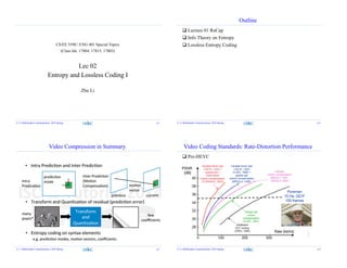
  • 1. CS/EE 5590 / ENG 401 Special Topics (Class Ids: 17804, 17815, 17803) Lec 02 Entropy and Lossless Coding I Zhu Li Z. Li Multimedia Communciation, 2016 Spring p.1 Outline  Lecture 01 ReCap  Info Theory on Entropy  Lossless Entropy Coding Z. Li Multimedia Communciation, 2016 Spring p.2 Video Compression in Summary Z. Li Multimedia Communciation, 2016 Spring p.3 Video Coding Standards: Rate-Distortion Performance  Pre-HEVC Z. Li Multimedia Communciation, 2016 Spring p.4
  • 2. PSS over managed IP networks  Managed mobile core IP networks Z. Li Multimedia Communciation, 2016 Spring p.5 MPEG DASH – OTT  HTTP Adaptive Streaming of Video Z. Li Multimedia Communciation, 2016 Spring p.6 Outline  Lecture 01 ReCap  Info Theory on Entropy  Self Info of an event  Entropy of the source  Relative Entropy  Mutual Info  Entropy Coding Thanks for SFU’s Prof. Jie Liang’s slides! Z. Li Multimedia Communciation, 2016 Spring p.7 Entropy and its Application Entropy coding: the last part of a compression system Losslessly represent symbols Key idea:  Assign short codes for common symbols  Assign long codes for rare symbols Question:  How to evaluate a compression method? o Need to know the lower bound we can achieve. o  Entropy Entropy coding QuantizationTransform Encoder 0100100101111 Z. Li Multimedia Communciation, 2016 Spring p.8
  • 3. Claude Shannon: 1916-2001  A distant relative of Thomas Edison  1932: Went to University of Michigan.  1937: Master thesis at MIT became the foundation of digital circuit design: o “The most important, and also the most famous, master's thesis of the century“  1940: PhD, MIT  1940-1956: Bell Lab (back to MIT after that)  1948: The birth of Information Theory o A mathematical theory of communication, Bell System Technical Journal. Z. Li Multimedia Communciation, 2016 Spring p.9 Axiom Definition of Information Information is a measure of uncertainty or surprise  Axiom 1:  Information of an event is a function of its probability: i(A) = f (P(A)). What’s the expression of f()?  Axiom 2:  Rare events have high information content  Water found on Mars!!!  Common events have low information content  It’s raining in Vancouver. Information should be a decreasing function of the probability: Still numerous choices of f().  Axiom 3:  Information of two independent events = sum of individual information: If P(AB)=P(A)P(B)  i(AB) = i(A) + i(B).  Only the logarithmic function satisfies these conditions. Z. Li Multimedia Communciation, 2016 Spring p.10 Self-information )(log )( 1 log)( xp xp xi bb  • Shannon’s Definition [1948]: • X: discrete random variable with alphabet {A1, A2, …, AN} • Probability mass function: p(x) = Pr{ X = x} • Self-information of an event X = x: If b = 2, unit of information is bit Self information indicates the number of bits needed to represent an event. 1 P(x) )(log xPb 0 Z. Li Multimedia Communciation, 2016 Spring p.11  Recall: the mean of a function g(X): Entropy is the expected self-information of the r.v. X:  The entropy represents the minimal number of bits needed to losslessly represent one output of the source. Entropy of a Random Variable  x xp xpXH )( 1 log)()( )g()())(()( xxpXgE xp   )(log )( 1 log )()( XpE Xp EH xpxp        Also write as H (p): function of the distribution of X, not the value of X. Z. Li Multimedia Communciation, 2016 Spring p.12
  • 4. Example P(X=0) = 1/2 P(X=1) = 1/4 P(X=2) = 1/8 P(X=3) = 1/8 Find the entropy of X. Solution: 1 ( ) ( )log ( ) 1 1 1 1 1 2 3 3 7 log 2 log 4 log8 log8 bits/sample. 2 4 8 8 2 4 8 8 4 x H X p x p x            Z. Li Multimedia Communciation, 2016 Spring p.13 Example A binary source: only two possible outputs: 0, 1  Source output example: 000101000101110101……  p(X=0) = p, p(X=1)= 1 – p. Entropy of X:  H(p) = p (-log2(p) ) + (1-p) (-log2(1-p))  H = 0 when p = 0 or p =1 oFixed output, no information  H is largest when p = 1/2 oHighest uncertainty oH = 1 bit in this case Properties:  H ≥ 0  H concave (proved later) 0 0.1 0.2 0.3 0.4 0.5 0.6 0.7 0.8 0.9 1 0 0.2 0.4 0.6 0.8 1 p Entropy Equal prob maximize entropy Z. Li Multimedia Communciation, 2016 Spring p.14 Joint entropy 1 1 2 2( , , )n np X i X i X i   • We can get better understanding of the source S by looking at a block of output X1X2…Xn: • The joint probability of a block of output:  Joint entropy 1 2 1 2 1 1 2 2 1 1 2 2 ( , , ) 1 ( , , )log ( , , )n n n n i i i n n H X X X p X i X i X i p X i X i X i               Joint entropy is the number of bits required to represent the sequence X1X2…Xn:  This is the lower bound for entropy coding.  ),...(log 1 nXXpE Z. Li Multimedia Communciation, 2016 Spring p.15 Conditional Entropy 1 ( ) ( | ) log log ( | ) ( , ) p y i x y p x y p x y   • Conditional Self-Information of an event X = x, given that event Y = y has occurred:  ( , ) ( | ) ( ) ( | ) ( ) ( | )log( ( | )) ( | ) ( )log( ( | )) ( , )log( ( | )) log( ( | ) x x y x y x y p x y H Y X p x H Y X x p x p y x p y x p y x p x p y x p x y p y x E p y x                 Conditional Entropy H(Y | X): Average cond. self-info. Remaining uncertainty about Y given the knowledge of X. Note: p(x | y), p(x, y) and p(y) are three different distributions: p1(x | y), p2(x, y) and p3(y). Z. Li Multimedia Communciation, 2016 Spring p.16
  • 5. Conditional Entropy Example: for the following joint distribution p(x, y), find H(Y | X). 1 2 3 4 1 1/8 1/16 1/32 1/32 2 1/16 1/8 1/32 1/32 3 1/16 1/16 1/16 1/16 4 1/4 0 0 0 Y X ( | ) ( ) ( | )log( ( | )) ( , )log( ( | )) x y x y H Y X p x p y x p y x p x y p y x      Need to find conditional prob p(y | x) ( , ) ( | ) ( ) p x y p y x p x  Need to find marginal prob p(x) first (sum columns). P(X): [ ½, ¼, 1/8, 1/8 ] >> H(X) = 7/4 bits P(Y): [ ¼ , ¼, ¼, ¼ ] >> H(Y) = 2 bits H(X|Y) = ∑ = ( | = ) = ¼ H(1/2 ¼ 1/8 1/8 ) + 1/4H(1/4, ½, 1/8 ,1/8) + 1/4H(1/4 ¼ ¼ ¼ ) + 1/4H(1 0 0 0) = 11/8 bits Z. Li Multimedia Communciation, 2016 Spring p.17 Chain Rule H(X, Y) = H(X) + H(Y|X) = H(Y) + H(X|Y) Proof: H(X) H(Y) H(X | Y) H(Y | X) Total area: H(X, Y)           x x yx y x y x y XYHXHXYHxpxp xypyxpxpyxp xypxpyxp yxpyxpYXH ).|()()|()(log)( )|(log),()(log),( )|()(log),( ),(log),(),( Simpler notation: )|()( ))|(log)((log)),((log),( XYHXH XYpXpEYXpEYXH   Z. Li Multimedia Communciation, 2016 Spring p.18 Conditional Entropy Example: for the following joint distribution p(x, y), find H(Y | X).  Indeed, H(X|Y) = H(X, Y) – H(Y)= 27/8 – 2 = 11/8 bits 1 2 3 4 1 1/8 1/16 1/32 1/32 2 1/16 1/8 1/32 1/32 3 1/16 1/16 1/16 1/16 4 1/4 0 0 0 Y X P(X): [ ½, ¼, 1/8, 1/8 ] >> H(X) = 7/4 bits P(Y): [ ¼ , ¼, ¼, ¼ ] >> H(Y) = 2 bits H(X|Y) = ∑ = ( | = ) = ¼ H(1/2 ¼ 1/8 1/8 ) + 1/4H(1/4, ½, 1/8 ,1/8) + 1/4H(1/4 ¼ ¼ ¼ ) + 1/4H(1 0 0 0) = 11/8 bits Z. Li Multimedia Communciation, 2016 Spring p.19 Chain Rule  H(X,Y) = H(X) + H(Y|X)  Corollary: H(X, Y | Z) = H(X | Z) + H(Y | X, Z) Note that: ( , | ) ( | , ) ( | )p x y z p y x z p x z (Multiply by p(z) at both sides, we get )( , , ) ( | , ) ( , )p x y z p y x z p x z ))|,((log)|,(log),,( )|,(log)|,()()|,( ZYXpEzyxpzyxp zyxpzyxpzpZYXH x y z x yz     Proof: ),|()|( )),|((log))|((log)|,( ZXYHZXH ZXYpEZXpEZYXH   Z. Li Multimedia Communciation, 2016 Spring p.20
  • 6. General Chain Rule General form of chain rule: )...|(),...,( 1,1 1 21 XXXHXXXH i n i in     The joint encoding of a sequence can be broken into the sequential encoding of each sample, e.g. H(X1, X2, X3)=H(X1) + H(X2|X1) + H(X3|X2, X1)  Advantages:  Joint encoding needs joint probability: difficult  Sequential encoding only needs conditional entropy, can use local neighbors to approximate the conditional entropy  context-adaptive arithmetic coding. Adding H(Z):  H(X, Y | Z) + H(z) = H(X, Y, Z) = H(z) + H(X | Z) + H(Y | X, Z) Z. Li Multimedia Communciation, 2016 Spring p.21 General Chain Rule ),...|()...|()(),...( 111211  nnn xxxpxxpxpxxpProof: .),...|( ),...|(log),...( ),...|(log),...( ),...|(log),...( ),...(log),...(),...( 1 11 1 ,...1 111 ,...1 11 1 1 ,...1 1 111 ,...1 111                      n i ii n i xnx iin xnx ii n i n xnx n i iin xnx nnn XXXH xxxpxxp xxxpxxp xxxpxxp xxpxxpXXH Z. Li Multimedia Communciation, 2016 Spring p.22 General Chain Rule 1 1( | ,... )i ip x x x  The complexity of the conditional probability grows as the increase of i. In many cases we can approximate the cond. probability with some nearest neighbors (contexts): 1 1 1( | ,... ) ( | ,... )i i i i L ip x x x p x x x    The low-dim cond prob is more manageable  How to measure the quality of the approximation?  Relative entropy 0 1 1 0 1 0 1 a b c b c a b c b a b c b a Z. Li Multimedia Communciation, 2016 Spring p.23 Relative Entropy – Cost of Coding with Wrong Distr Also known as Kullback Leibler (K-L) Distance, Information Divergence, Information Gain A measure of the “distance” between two distributions:  In many applications, the true distribution p(X) is unknown, and we only know an estimation distribution q(X)  What is the inefficiency in representing X? o The true entropy: o The actual rate: o The difference:         )( )( log )( )( log)()||( Xq Xp E xq xp xpqpD p x 1 ( )log ( ) x R p x p x  2 ( )log ( ) x R p x q x  2 1 ( || )R R D p q  Z. Li Multimedia Communciation, 2016 Spring p.24
  • 7. Relative Entropy Properties:         )( )( log )( )( log)()||( Xq Xp E xq xp xpqpD p x ( || ) 0.D p q  ( || ) 0 if and only if q = p.D p q   What if p(x)>0, but q(x)=0 for some x?  D(p||q)=∞  Caution: D(p||q) is not a true distance  Not symmetric in general: D(p || q) ≠ D(q || p)  Does not satisfy triangular inequality. Proved later. Z. Li Multimedia Communciation, 2016 Spring p.25 Relative Entropy How to make it symmetric?  Many possibilities, for example:   1 ( || ) ( || ) 2 D p q D q p ( || ) ( || )D p q D q p  can be useful for pattern classification. )||( 1 )||( 1 pqDqpD  Z. Li Multimedia Communciation, 2016 Spring p.26 Mutual Information i (x | y): conditional self-information )()( ),( log )( )|( log)|()();( ypxp yxp xp yxp yxixiyxi  Note: i(x; y) can be negative, if p(x | y) < p(x).  Mutual information between two events: i(x | y) = -log p(x | y)  A measure of the amount of information that one event contains about another one.  or the reduction in the uncertainty of one event due to the knowledge of the other. Z. Li Multimedia Communciation, 2016 Spring p.27 Mutual Information I(X; Y): Mutual information between two random variables:   ( , ) ( , ) ( ; ) ( , ) ( ; ) ( , )log ( ) ( ) ( , ) D ( , ) || ( ) ( ) log ( ) ( ) x y x y p x y p x y I X Y p x y i x y p x y p x p y p X Y p x y p x p y E p X p Y             But it is symmetric: I(X; Y) = I(Y; X)  Mutual information is a relative entropy:  If X, Y are independent: p(x, y) = p(x) p(y)  I (X; Y) = 0  Knowing X does not reduce the uncertainty of Y. Different from i(x; y), I(X; Y) >=0 (due to averaging) Z. Li Multimedia Communciation, 2016 Spring p.28
  • 8. Entropy and Mutual Information ( , ) ( | ) ( ; ) ( , )log ( , )log ( ) ( ) ( ) ( , )log ( | ) ( , )log ( ) ( ) ( | ) x y x y x y x y p x y p x y I X Y p x y p x y p x p y p x p x y p x y p x y p x H X H X Y           2. Similarly: ( ; ) ( ) ( | )I X Y H Y H Y X  1. 3. I(X; Y) = H(X) + H(Y) – H(X, Y) Proof: Expand the definition: ( ; ) ( ) ( | )I X Y H X H X Y    ),()()( )(log)(log),(log),();( YXHYHXH ypxpyxpyxpYXI x y    Z. Li Multimedia Communciation, 2016 Spring p.29 Entropy and Mutual Information H(X) H(Y) I(X; Y)H(X | Y) H(Y | X) Total area: H(X, Y) It can be seen from this figure that I(X; X) = H(X): Proof: Let X = Y in I(X; Y) = H(X) + H(Y) – H(X, Y), or in I(X; Y) = H(X) – H(X | Y) (and use H(X|X)=0). Z. Li Multimedia Communciation, 2016 Spring p.30 Application of Mutual Information a b c b c a b c b a b c b a Mutual information can be used in the optimization of context quantization. Example: If each neighbor has 26 possible values (a to z), then 5 neighbors have 265 combinations:  too many cond probs to estimate. To reduce the number, can group similar data pattern together  context quantization   1 1 1 1( | ,... ) | ,...i i i ip x x x p x f x x  Z. Li Multimedia Communciation, 2016 Spring p.31 Application of Mutual Information We need to design the function f( ) to minimize the conditional entropy   1 1 1 1( | ,... ) | ,...i i i ip x x x p x f x x  )...|(),...,( 1,1 1 21 XXXHXXXH i n i in    ( | ) ( ) ( ; )H X Y H X I X Y But The problem is equivalent to maximizing the mutual information between Xi and f(x1, … xi-1). ))...(|( 1,1 XXfXH ii  For further info: Liu and Karam, Mutual Information-Based Analysis of JPEG2000 Contexts, IEEE Trans Image Processing, VOL. 14, NO. 4, APRIL 2005, pp. 411-422. Z. Li Multimedia Communciation, 2016 Spring p.32
  • 9. Outline  Lecture 01 ReCap  Info Theory on Entropy  Entropy Coding  Prefix Coding  Kraft-McMillan Inequality  Shannon Codes Z. Li Multimedia Communciation, 2016 Spring p.33 Variable Length Coding Design the mapping from source symbols to codewords Lossless mapping Different codewords may have different lengths Goal: minimizing the average codeword length The entropy is the lower bound. Z. Li Multimedia Communciation, 2016 Spring p.34 Classes of Codes Non-singular code: Different inputs are mapped to different codewords (invertible). Uniquely decodable code: any encoded string has only one possible source string, but may need delay to decode. Prefix-free code (or simply prefix, or instantaneous): No codeword is a prefix of any other codeword.  The focus of our studies.  Questions: o Characteristic? o How to design? o Is it optimal? All codes Non-singular codes Uniquely decodable codes Prefix-free codes Z. Li Multimedia Communciation, 2016 Spring p.35 Prefix Code  Examples X Singular Non-singular, But not uniquely decodable Uniquely decodable, but not prefix-free Prefix-free 1 0 0 0 0 2 0 010 01 10 3 0 01 011 110 4 0 10 0111 111 Need punctuation ……01011… Need to look at next bit to decode previous code. Z. Li Multimedia Communciation, 2016 Spring p.36
  • 10. Carter-Gill’s Conjecture [1974] Carter-Gill’s Conjecture [1974]  Every uniquely decodable code can be replaced by a prefix-free code with the same set of codeword compositions.  So we only need to study prefix-free code. Z. Li Multimedia Communciation, 2016 Spring p.37 Prefix-free Code Can be uniquely decoded. No codeword is a prefix of another one. Also called prefix code Goal: construct prefix code with minimal expected length. Can put all codewords in a binary tree: 0 1 0 1 0 1 0 10 110 111 Root node leaf node Internal node  Prefix-free code contains leaves only.  How to express the requirement mathematically? Z. Li Multimedia Communciation, 2016 Spring p.38 Kraft-McMillan Inequality 12 1   N i li • The codeword lengths li, i=1,…N of a prefix code over an alphabet of size D(=2) satisfies the inequality Conversely, if a set of {li} satisfies the inequality above, then there exists a prefix code with codeword lengths li, i=1,…N.  The characteristic of prefix-free codes: Z. Li Multimedia Communciation, 2016 Spring p.39 Kraft-McMillan Inequality 2212 11 L N i lL N i l ii        Consider D=2: expand the binary code tree to full depth L = max(li) 0 10 110 111  Number of nodes in the last level:  Each code corresponds to a sub-tree:  The number of off springs in the last level:  K-M inequality: # of L-th level offsprings of all codes is less than 2^L ! ilL 2 L 2 L = 3 Example: {0, 10, 110, 111} Z. Li Multimedia Communciation, 2016 Spring p.40 2^3=8 {4, 2, 0, 0}
  • 11. Kraft-McMillan Inequality 0 10 110 111 11 Invalid code: {0, 10, 11, 110, 111} Leads to more than 2^L offspring: 12> 23 12 1     i li  K-M inequality: Z. Li Multimedia Communciation, 2016 Spring p.41 Extended Kraft Inequality Countably infinite prefix code also satisfies the Kraft inequality:  Has infinite number of codewords. Example:  0, 10, 110, 1110, 11110, 111……10, …… (Golomb-Rice code, next lecture)  Each codeword can be mapped to a subinterval in [0, 1] that is disjoint with others (revisited in arithmetic coding) 1 1     i li D ) 0 ) 10 ) 0 0.5 0.75 0.875 1 110 …… Z. Li Multimedia Communciation, 2016 Spring p.42 0 10 110 …. L = 3 Optimal Codes (Advanced Topic) How to design the prefix code with the minimal expected length? Optimization Problem: find {li} to 1.. min    i i l ii l Dts lp  Lagrangian solution:  Ignore the integer codeword length constraint for now  Assume equality holds in the Kraft inequality    il ii DlpJ Minimize Z. Li Multimedia Communciation, 2016 Spring p.43 Optimal Codes    il ii DlpJ    0lnLet     il i i DDp l J   D p D ili ln  1intongSubstituti   il D Dln 1  i l pD i  or iDi pl log- *  The optimal codeword length is the self-information of an event. Expected codeword length: )(log* XHpplpL DiDiii    Entropy of X ! Z. Li Multimedia Communciation, 2016 Spring p.44
  • 12. Optimal Code Theorem: The expected length L of any prefix code is greater or equal to the entropy with equality holds iff is not integer in general.iDi p-l log *  ( )DL H X  Proof: ( ) log log log logi i D i i i D i l i i D i D i i D l L H X p l p p p p D p p p D            This reminds us the definition of relative entropy D(p ||q), but we need to normalize D-li. i l pD i  Z. Li Multimedia Communciation, 2016 Spring p.45 Pi is Diadic, ½, ¼, 1/8, 1/16… Optimal Code  Let distribution be diadic, i.e, = / ∑ because D(p||q) >= 0, and 1 1 for prefix code.i N l i D   The equality holds iff both terms are 0:  i l pD i  or logD ip is an integer. Z. Li Multimedia Communciation, 2016 Spring p.46 − = log = log + log 1/( ) = ( | + log 1 ∑ Optimal Code D-adic: a probability distribution is called D-adic with respect to D if each probability is equal to D-n for some integer n:  Example: {1/2, 1/4, 1/8, 1/8} Therefore the optimality can be achieved by prefix code iff the distribution is D-adic.  Previous example:  Possible codewords: o {0, 10, 110, 111} log {1,2,3,3}D ip  Z. Li Multimedia Communciation, 2016 Spring p.47 Shannon Code: Bounds on Optimal Code is not integer in general. iDi p-l log *  Practical codewords have to be integer.        i Di p l 1 logShannon Code: Is this a valid prefix code? Check Kraft inequality .1 1 log 1 log           i ppl pDDD i D i D i 1 1 log 1 log  i Di i D p l p       i Di p l 1 log 1)()(  XHLXH DD Yes ! This is just one choice. May not be optimal (see example later) Z. Li Multimedia Communciation, 2016 Spring p.48
  • 13. Optimal Code The optimal code with integer lengths should be better than Shannon code 1)()( *  XHLXH DD  To reduce the overhead per symbol:  Encode a block of symbols {x1, x2, …, xn} together  ),...,,( 1 ),...,,(),...,,( 1 212121 nnnn xxxlE n xxxlxxxp n L     1),...,,(),...,,(),...,,( 212121  nnn XXXHxxxlEXXXH Assume i.i.d. samples: )(),...,,( 21 XnHXXXH n  n XHLXH n 1 )()(  )(XHLn  if stationary. (entropy rate) Z. Li Multimedia Communciation, 2016 Spring p.49 Optimal Code Impact of wrong pdf: what’s the penalty if the pdf we use is different from the true pdf? True pdf: p(x) Codeword length: l(x) Estimated pdf: q(x) Expected length: Epl(X) 1)||()()()||()(  qpDpHXlEqpDpH p Proof: assume Shannon code        )( 1 log)( xq xl               1 )( 1 log)( )( 1 log)()( xq xp xq xpXlEp 1)||()(1 )( 1 )( )( log)(                 qpDXH xpxq xp xp The lower bound is derived similarly. Z. Li Multimedia Communciation, 2016 Spring p.50 Shannon Code is not optimal Example:  Binary r.v. X: p(0)=0.9999, p(1)=0.0001. Entropy: 0.0015 bits/sample Assign binary codewords by Shannon code:        )( 1 log)( xp xl .1 9999.0 1 log2     .14 0001.0 1 log2        Expected length: 0.9999 x 1+ 0.0001 x 14 = 1.0013.  Within the range of [H(X), H(X) + 1].  But we can easily beat this by the code {0, 1}  Expected length: 1. Z. Li Multimedia Communciation, 2016 Spring p.51 Q&A Z. Li Multimedia Communciation, 2016 Spring p.52