2. Review: Mathematical Basics
Mathematical Description of Source Coding
encoder decoder
message bitstream
...0011010100...
message
Transmission of new information to receiver
Message is unknown by receiver
Source can be modeled as a random process
Modeling of information sources as random processes
Description using mathematical framework of probability theory
Requires reasonable assumptions with respect to source of information
Characterization of performance by probabilistic averages
Basis for mathematical theory of communication
Heiko Schwarz (Freie Universität Berlin) — Data Compression: Variable-Length Codes 2 / 63
3. Review: Mathematical Basics / Probability
Probability Axioms
Random experiment: Any experiment with uncertain outcome ζ
Sample space O: Union of all possible outcomes ζ (also called certain event O)
Event A: Union of zero or more possible outcomes ζ (A ⊆ O)
Probability P(A): Measure P(A) assigned to events A of a random experiment
that satisfies the following axioms (Kolmogorov):
1 Probabilities are non-negative real numbers
P(A) ≥ 0, ∀A ⊆ O
2 Certain event O has a probability equal to 1
P(O) = 1
3 Probability of two disjoint events A and B
A ∩ B = ∅ =⇒ P(A ∪ B) = P(A) + P(B)
Heiko Schwarz (Freie Universität Berlin) — Data Compression: Variable-Length Codes 3 / 63
4. Review: Mathematical Basics / Probability
Conditional Probability and Independence of Events
Conditional Probability P(A | B) (Kolmogorov)
Probability of an event A given that another event B has occured
P(A | B) =
P(A ∩ B)
P(B)
, for P(B) > 0
Bayes’ Theorem
P(A | B) = P(B | A) ·
P(A)
P(B)
, for P(A) > 0, P(B) > 0
Independence of Events
Two events A and B are said to be independent if and only if
P(A ∩ B) = P(A) · P(B)
For independent events A and B, with P(B) > 0, we have
P(A | B) = P(A)
Heiko Schwarz (Freie Universität Berlin) — Data Compression: Variable-Length Codes 4 / 63
5. Review: Mathematical Basics / Probability
Probability Estimation
Empirical Probability
Repeatable random experiment
Relative frequency of an event A in N trials
N(A)
N
=
number of trials in which A was observed
number of total trials
Empirical probability
P(A) = lim
N→∞
N(A)
N
Practical Probability Estimation
Use the approximation
P(A) =
N(A)
N
Estimation quality depends on the number of trials N
Heiko Schwarz (Freie Universität Berlin) — Data Compression: Variable-Length Codes 5 / 63
6. Review: Mathematical Basics / Discrete Random Variables
Random Variables
Random Variable
Function X(ζ) of the sample space O that assigns a real value x = X(ζ)
to each possible outcome ζ ∈ O of a random experiment
A random variable may take ...
a finite number of values
a countable infinite number of values
an uncountable number of values
Examples for Random Variables
Dice roll: Number on top face of the die (finite)
Roulette: Number of pocket the ball lands (finite)
Microphone: Voltage on output of microphone (uncountable)
Digital signal: Value of next sample (finite)
Heiko Schwarz (Freie Universität Berlin) — Data Compression: Variable-Length Codes 6 / 63
7. Review: Mathematical Basics / Discrete Random Variables
Cumulative Distribution Function
Cumulative Distribution Function (cdf)
Cumulative distribution function FX (x) of a random variable X
FX (s) = P(X ≤ x) = P( {ζ : X(ζ) ≤ x} )
FX (x) is also referred to as distribution of the random variable X
Joint and Conditional Cumulative Distribution Functions
Joint cdf of two random variables X and Y
FXY (x, y) = P(X ≤ x, Y ≤ y)
Conditional cdf of a random variable X given another random variable Y
FX|Y (x | y) = P(X ≤ x | Y ≤ y) =
P(X ≤ x, Y ≤ y)
P(Y ≤ y)
=
FXY (x, y)
FY (y)
Heiko Schwarz (Freie Universität Berlin) — Data Compression: Variable-Length Codes 7 / 63
8. Review: Mathematical Basics / Discrete Random Variables
Examples: Cumulative Distribution Functions
x
FX (x)
Continuous function
Random variable X
can take all values
inside one or more
non-zero intervals
Continuous
random variable
x
FX (x)
Staircase function
Random variable X
can only take a
countable number
of values
Discrete
random variable
x
FX (x)
Mixed type
Random variable X
can take all values
inside one or more
non-zero intervals and
a countable number of
additional values
Heiko Schwarz (Freie Universität Berlin) — Data Compression: Variable-Length Codes 8 / 63
9. Review: Mathematical Basics / Discrete Random Variables
Discrete Random Variables
Discrete Random Variables
A random variable X is called a discrete random variable
if and only if its cdf FX (x) is a staircase function
Discrete random variables X can only take values of a countable alphabet
AX = {x0, x1, x2, · · · }
Examples for Discrete Random Variables
Result of a coin toss: AX = {0, 1} (0: ”head”, 1: ”tail”)
Number on top face of the die: AX = {1, 2, 3, 4, 5, 6}
Sample in an 8-bit gray image: AX = {0, 1, 2, · · · , 255}
Sample in a 16-bit audio signal: AX = {−32768, −32767, · · · , −1, 0, 1, · · · , 32766, 32767}
Heiko Schwarz (Freie Universität Berlin) — Data Compression: Variable-Length Codes 9 / 63
10. Review: Mathematical Basics / Discrete Random Variables
Probability Mass Function
Probability Mass Function (pmf)
Probability mass function pX (x) of discrete random variable X with alphabet AX
pX (x) = P(X = x) = P( {ζ ∈ O : X(ζ) = x} ) for x ∈ AX
Pmfs have the following property
X
x∈AX
pX (x) = P(O) = 1
Joint and Conditional Probability Mass Functions
Joint pmf of two discrete random variables X and Y
pXY (x, y) = P(X = x, Y = y)
Conditional pmf of a discrete random variable X given another discrete random variable Y
pX|Y (x | y) = P(X = x | Y = y) =
P(X = x, Y = y)
P(Y = y)
=
pXY (x, y)
pY (y)
Heiko Schwarz (Freie Universität Berlin) — Data Compression: Variable-Length Codes 10 / 63
11. Review: Mathematical Basics / Discrete Random Variables
Examples for Discrete Distributions
Uniform Binomial Geometric
pk = 1
M
(0 ≤ k < M)
pk = n
k
pk
(1 − p)n−k
(0 ≤ k ≤ n)
pk = (1 − p)k
p
(k ≥ 0)
xk
pk
xk
pk
xk
pk
x
FX (x)
x
FX (x)
x
FX (x)
Heiko Schwarz (Freie Universität Berlin) — Data Compression: Variable-Length Codes 11 / 63
12. Review: Mathematical Basics / Discrete Random Variables
Example: 1D Histogram for English Text
x
N(x)
Large English text
(ca. 6 million characters)
THE ADVENTURES OF
SHERLOCK HOLMES
BY
SIR ARTHUR CONAN DOYLE
CONTENTS
I. A Scandal in Bohemia
II. The Red-Headed League
III. A Case of Identity
IV. The Boscombe Valley Mystery
V. The Five Orange Pips
VI. The Man with the Twisted Lip
VII. The Adventure of the Blue Carbuncle
VIII. The Adventure of the Speckled Band
IX. The Adventure of the Engineer’s Thumb
X. The Adventure of the Noble Bachelor
XI. The Adventure of the Beryl Coronet
XII. The Adventure of the Copper Beeches
...
Heiko Schwarz (Freie Universität Berlin) — Data Compression: Variable-Length Codes 12 / 63
13. Review: Mathematical Basics / Discrete Random Variables
Example: 1D Histogram for Single-Channel Audio
x
N(x)
Queen “Bohemian Rhapsody”
(ca. 15 million samples)
Heiko Schwarz (Freie Universität Berlin) — Data Compression: Variable-Length Codes 13 / 63
14. Review: Mathematical Basics / Discrete Random Variables
Example: 1D Histogram for Natural Gray-Level Images
x
N(x)
15 test images (each 768×512)
Heiko Schwarz (Freie Universität Berlin) — Data Compression: Variable-Length Codes 14 / 63
15. Review: Mathematical Basics / Expected Values
Expected Values
Expected Values
Expected value of a function g(X) of a discrete random variable X with alphabet AX
E{ g(X) } = EX { g(X) } =
X
∀x∈AX
g(x) pX (x)
Expected value of function g(X, Y ) of two discrete random variable X and Y
E{ g(X, Y ) } = EXY { g(X, Y ) } =
X
x,y
g(x, y) pXY (x, y)
Conditional Expected Values
Expected value of function g(X) given an event B or another random variable Y
E{ g(X) | B } =
X
x
g(x) pX|B(x | B) for P(B) 0
E{ g(X) | Y } =
X
x
g(x) pX|Y (x | Y ) (another random variable)
Heiko Schwarz (Freie Universität Berlin) — Data Compression: Variable-Length Codes 15 / 63
16. Review: Mathematical Basics / Expected Values
Properties of Expected Values
Important Properties
Linearity of expected values
E{ a X + b Y } = a · E{ X } + b · E{ Y }
For independent random variables X and Y
E{ XY } = E{ X } E{ Y }
Iterative expectation rule
E{ E{ g(X) | Y } } = E{ g(X) }
Heiko Schwarz (Freie Universität Berlin) — Data Compression: Variable-Length Codes 16 / 63
17. Review: Mathematical Basics / Expected Values
Important Expected Values
Mean µX of a random variable X
µX = E{ X } =
X
x
x · pX (x)
Variance σ2
X of a random variable X
σ2
X = E
n
(X − E{ X })2
o
=
X
x
(x − µX )2
· pX (x)
Covariance σ2
XY of two random variables X and Y , and correlation coefficient φXY
σ2
XY = E
n
(X − E{ X }) (Y − E{ Y })
o
=
X
x,y
(x − µx )(y − µy ) · pXY (x, y)
φXY =
σ2
XY
p
σ2
X · σ2
Y
Heiko Schwarz (Freie Universität Berlin) — Data Compression: Variable-Length Codes 17 / 63
18. Review: Mathematical Basics / Discrete Random Processes
Random Processes
Discrete-Time Random Process
Series of random experiments at time instants tn, with n = 0, 1, 2, · · ·
For each experiment: Random variable Xn = X(tn)
Random process: Series of random variables
X = {X0, X1, X2, · · · } = {Xn}
Discrete-Time Discrete-Amplitude Random Process
Random variables Xn are discrete random variables
Each random variable Xn has an alphabet An
Type of random processes we consider for lossless coding
Heiko Schwarz (Freie Universität Berlin) — Data Compression: Variable-Length Codes 18 / 63
19. Review: Mathematical Basics / Discrete Random Processes
Statistical Properties of Random Processes
Characterization of Statistical Properties
Consider N-dimensional random vector
X
(N)
k = {Xk , Xk+1, · · · , Xk+N−1}
N-th order joint cdf
F
(N)
k (x) = P
X
(N)
k ≤ x
= P(Xk ≤ x0, Xk+1 ≤ x1, · · · , Xk+N−1 ≤ xN−1)
N-th order joint pmf
p
(N)
k (x) = P
X
(N)
k = x
= P(Xk = x0, Xk+1 = x1, · · · , Xk+N−1 = xN−1)
Also: Conditional cdfs and conditional pmfs
Heiko Schwarz (Freie Universität Berlin) — Data Compression: Variable-Length Codes 19 / 63
20. Review: Mathematical Basics / Discrete Random Processes
Models for Random Processes
Stationary Random Processes
Statistical properties are invariant to a shift in time
In this course: Typically restrict our considerations to stationary processes
Memoryless Random Processes
All random variables Xn are independent of each other
Independent and Identically Distributed (IID) Random Processes
Random processes that are stationary and memoryless
Valid model for fair games: Dice roll or roulette
Markov Processes
Markov property: Future outcomes do only depend on present outcome, but not on past outcomes
P(Xn = sn | Xn−1 = xn−1, Xn−2 = xn−2, · · · ) = P(Xn = xn | Xn−1 = xn−1)
Simple model for random processes with memory
Heiko Schwarz (Freie Universität Berlin) — Data Compression: Variable-Length Codes 20 / 63
21. Review: Mathematical Basics / Discrete Random Processes
Stationary Discrete Markov Processes
Stationary Discrete Random Process with Markov Property
Simple model for investigating coding of sources with memory
Statistical properties are completly specified by 1-st order conditional cdf or pmf
F(xn | xn−1) = P(Xn ≤ xn | Xn−1 ≤ xn−1)
p(xn | xn−1) = P(Xn = xn | Xn−1 = xn−1)
Extension: N-th order stationary discrete Markov processes
Example: Stationary Discrete Markov Process
AX = {a, b, c}
conditional pmf
p(xn | xn−1)
xn p(xn | a) p(xn | b) p(xn | c)
a 0.90 0.15 0.25
b 0.05 0.80 0.15
c 0.05 0.05 0.60
Question:
What is the
marginal
pmf pX (x) ?
Heiko Schwarz (Freie Universität Berlin) — Data Compression: Variable-Length Codes 21 / 63
22. Review: Mathematical Basics / Discrete Random Processes
Example: 2D Histogram for English Text
xn
xn−1
N(xn−1, xn)
joint histogram of two adjacent characters Large English upper-case text
(ca. 6 million characters)
THE ADVENTURES OF
SHERLOCK HOLMES
BY
SIR ARTHUR CONAN DOYLE
CONTENTS
I. A SCANDAL IN BOHEMIA
II. THE RED-HEADED LEAGUE
III. A CASE OF IDENTITY
IV. THE BOSCOMBE VALLEY MYSTERY
V. THE FIVE ORANGE PIPS
VI. THE MAN WITH THE TWISTED LIP
VII. THE ADVENTURE OF THE BLUE CARBUNCLE
VIII. THE ADVENTURE OF THE SPECKLED BAND
IX. THE ADVENTURE OF THE ENGINEER’S THUMB
X. THE ADVENTURE OF THE NOBLE BACHELOR
XI. THE ADVENTURE OF THE BERYL CORONET
XII. THE ADVENTURE OF THE COPPER BEECHES
...
Heiko Schwarz (Freie Universität Berlin) — Data Compression: Variable-Length Codes 22 / 63
23. Review: Mathematical Basics / Discrete Random Processes
Example: 2D Histogram for Single-Channel Audio
xn
xn−1
N(xn−1, xn)
joint histogram
of two directly
successive samples
Queen “Bohemian Rhapsody”
(ca. 15 million samples)
Heiko Schwarz (Freie Universität Berlin) — Data Compression: Variable-Length Codes 23 / 63
24. Review: Mathematical Basics / Discrete Random Processes
Example: 2D Histogram for Natural Gray-Level Images
xn
xn−1
N(xn−1, xn)
joint histogram
of two horizontally
adjacent samples
15 test images (each 768×512)
Heiko Schwarz (Freie Universität Berlin) — Data Compression: Variable-Length Codes 24 / 63
25. Review: Mathematical Basics / Summary
Summary of Mathematical Basics
Probability
Axiomatic definition, empirical probability
Conditional probability and independence of events
Discrete Random Variables
Can take only values of a countable alphabet
Cumulative distribution function (cdf): Staircase function
Probability mass function (pmf)
Expected values: Mean, variance, covariance
Discrete Random Variables
Sequence of random variables: Model for sources of digital signals
Types of random processes: Stationary, memoryless, iid, Markov
Stationary discrete Markov processes: Simple model for sources with memory
Heiko Schwarz (Freie Universität Berlin) — Data Compression: Variable-Length Codes 25 / 63
26. Scalar Variable-Length Codes
Morse Code (first version around 1837)
Heiko Schwarz (Freie Universität Berlin) — Data Compression: Variable-Length Codes 26 / 63
27. Scalar Variable-Length Codes
Example: Variable-Length Coding for Scalars
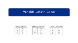
Symbol alphabet: A = {A, B, M, N}
Heiko Schwarz (Freie Universität Berlin) — Data Compression: Variable-Length Codes 27 / 63
28. Scalar Variable-Length Codes
Example: Variable-Length Coding for Scalars
Symbol alphabet: A = {A, B, M, N}
code A
letter codeword
A 00
B 01
M 10
N 11
Heiko Schwarz (Freie Universität Berlin) — Data Compression: Variable-Length Codes 27 / 63
29. Scalar Variable-Length Codes
Example: Variable-Length Coding for Scalars
Symbol alphabet: A = {A, B, M, N}
code A
letter codeword
A 00
B 01
M 10
N 11
Example message: s = “BANANAMAN”
Heiko Schwarz (Freie Universität Berlin) — Data Compression: Variable-Length Codes 27 / 63
30. Scalar Variable-Length Codes
Example: Variable-Length Coding for Scalars
Symbol alphabet: A = {A, B, M, N}
code A
letter codeword
A 00
B 01
M 10
N 11
Example message: s = “BANANAMAN”
Bitstream (code A): b = “010011001100100011” (18 bits)
Heiko Schwarz (Freie Universität Berlin) — Data Compression: Variable-Length Codes 27 / 63
31. Scalar Variable-Length Codes
Example: Variable-Length Coding for Scalars
Symbol alphabet: A = {A, B, M, N}
code A
letter codeword
A 00
B 01
M 10
N 11
code B
letter codeword
A 010
B 100
M 10
N 0
Example message: s = “BANANAMAN”
Bitstream (code A): b = “010011001100100011” (18 bits)
Heiko Schwarz (Freie Universität Berlin) — Data Compression: Variable-Length Codes 27 / 63
32. Scalar Variable-Length Codes
Example: Variable-Length Coding for Scalars
Symbol alphabet: A = {A, B, M, N}
code A
letter codeword
A 00
B 01
M 10
N 11
code B
letter codeword
A 010
B 100
M 10
N 0
Example message: s = “BANANAMAN”
Bitstream (code A): b = “010011001100100011” (18 bits)
Bitstream (code B): b = “10001000100010100100” (20 bits)
Heiko Schwarz (Freie Universität Berlin) — Data Compression: Variable-Length Codes 27 / 63
33. Scalar Variable-Length Codes
Example: Variable-Length Coding for Scalars
Symbol alphabet: A = {A, B, M, N}
code A
letter codeword
A 00
B 01
M 10
N 11
code B
letter codeword
A 010
B 100
M 10
N 0
code C
letter codeword
A 0
B 110
M 111
N 10
Example message: s = “BANANAMAN”
Bitstream (code A): b = “010011001100100011” (18 bits)
Bitstream (code B): b = “10001000100010100100” (20 bits)
Heiko Schwarz (Freie Universität Berlin) — Data Compression: Variable-Length Codes 27 / 63
34. Scalar Variable-Length Codes
Example: Variable-Length Coding for Scalars
Symbol alphabet: A = {A, B, M, N}
code A
letter codeword
A 00
B 01
M 10
N 11
code B
letter codeword
A 010
B 100
M 10
N 0
code C
letter codeword
A 0
B 110
M 111
N 10
Example message: s = “BANANAMAN”
Bitstream (code A): b = “010011001100100011” (18 bits)
Bitstream (code B): b = “10001000100010100100” (20 bits)
Bitstream (code C): b = “1100100100111010” (16 bits)
Heiko Schwarz (Freie Universität Berlin) — Data Compression: Variable-Length Codes 27 / 63
35. Scalar Variable-Length Codes
Example: Variable-Length Coding for Scalars
Symbol alphabet: A = {A, B, M, N}
code A
letter codeword
A 00
B 01
M 10
N 11
code B
letter codeword
A 010
B 100
M 10
N 0
code C
letter codeword
A 0
B 110
M 111
N 10
Example message: s = “BANANAMAN”
Bitstream (code A): b = “010011001100100011” (18 bits)
Bitstream (code B): b = “10001000100010100100” (20 bits)
Bitstream (code C): b = “1100100100111010” (16 bits)
Goal: Minimize average codeword length
¯
` = E{ `(S) } =
X
k
pk · `k
Heiko Schwarz (Freie Universität Berlin) — Data Compression: Variable-Length Codes 27 / 63
36. Scalar Variable-Length Codes
Example: Variable-Length Coding for Scalars
Symbol alphabet: A = {A, B, M, N}
code A
letter codeword
A 00
B 01
M 10
N 11
code B
letter codeword
A 010
B 100
M 10
N 0
code C
letter codeword
A 0
B 110
M 111
N 10
Decoding:
Heiko Schwarz (Freie Universität Berlin) — Data Compression: Variable-Length Codes 28 / 63
37. Scalar Variable-Length Codes
Example: Variable-Length Coding for Scalars
Symbol alphabet: A = {A, B, M, N}
code A
letter codeword
A 00
B 01
M 10
N 11
code B
letter codeword
A 010
B 100
M 10
N 0
code C
letter codeword
A 0
B 110
M 111
N 10
Decoding:
Code A: b = “010011001100100011“ s = “
Heiko Schwarz (Freie Universität Berlin) — Data Compression: Variable-Length Codes 28 / 63
38. Scalar Variable-Length Codes
Example: Variable-Length Coding for Scalars
Symbol alphabet: A = {A, B, M, N}
code A
letter codeword
A 00
B 01
M 10
N 11
code B
letter codeword
A 010
B 100
M 10
N 0
code C
letter codeword
A 0
B 110
M 111
N 10
Decoding:
Code A: b = “010011001100100011“ s = “B
Heiko Schwarz (Freie Universität Berlin) — Data Compression: Variable-Length Codes 28 / 63
39. Scalar Variable-Length Codes
Example: Variable-Length Coding for Scalars
Symbol alphabet: A = {A, B, M, N}
code A
letter codeword
A 00
B 01
M 10
N 11
code B
letter codeword
A 010
B 100
M 10
N 0
code C
letter codeword
A 0
B 110
M 111
N 10
Decoding:
Code A: b = “010011001100100011“ s = “BA
Heiko Schwarz (Freie Universität Berlin) — Data Compression: Variable-Length Codes 28 / 63
40. Scalar Variable-Length Codes
Example: Variable-Length Coding for Scalars
Symbol alphabet: A = {A, B, M, N}
code A
letter codeword
A 00
B 01
M 10
N 11
code B
letter codeword
A 010
B 100
M 10
N 0
code C
letter codeword
A 0
B 110
M 111
N 10
Decoding:
Code A: b = “010011001100100011“ s = “BAN
Heiko Schwarz (Freie Universität Berlin) — Data Compression: Variable-Length Codes 28 / 63
41. Scalar Variable-Length Codes
Example: Variable-Length Coding for Scalars
Symbol alphabet: A = {A, B, M, N}
code A
letter codeword
A 00
B 01
M 10
N 11
code B
letter codeword
A 010
B 100
M 10
N 0
code C
letter codeword
A 0
B 110
M 111
N 10
Decoding:
Code A: b = “010011001100100011“ s = “BANA
Heiko Schwarz (Freie Universität Berlin) — Data Compression: Variable-Length Codes 28 / 63
42. Scalar Variable-Length Codes
Example: Variable-Length Coding for Scalars
Symbol alphabet: A = {A, B, M, N}
code A
letter codeword
A 00
B 01
M 10
N 11
code B
letter codeword
A 010
B 100
M 10
N 0
code C
letter codeword
A 0
B 110
M 111
N 10
Decoding:
Code A: b = “010011001100100011“ s = “BANAN
Heiko Schwarz (Freie Universität Berlin) — Data Compression: Variable-Length Codes 28 / 63
43. Scalar Variable-Length Codes
Example: Variable-Length Coding for Scalars
Symbol alphabet: A = {A, B, M, N}
code A
letter codeword
A 00
B 01
M 10
N 11
code B
letter codeword
A 010
B 100
M 10
N 0
code C
letter codeword
A 0
B 110
M 111
N 10
Decoding:
Code A: b = “010011001100100011“ s = “BANANA
Heiko Schwarz (Freie Universität Berlin) — Data Compression: Variable-Length Codes 28 / 63
44. Scalar Variable-Length Codes
Example: Variable-Length Coding for Scalars
Symbol alphabet: A = {A, B, M, N}
code A
letter codeword
A 00
B 01
M 10
N 11
code B
letter codeword
A 010
B 100
M 10
N 0
code C
letter codeword
A 0
B 110
M 111
N 10
Decoding:
Code A: b = “010011001100100011“ s = “BANANAM
Heiko Schwarz (Freie Universität Berlin) — Data Compression: Variable-Length Codes 28 / 63
45. Scalar Variable-Length Codes
Example: Variable-Length Coding for Scalars
Symbol alphabet: A = {A, B, M, N}
code A
letter codeword
A 00
B 01
M 10
N 11
code B
letter codeword
A 010
B 100
M 10
N 0
code C
letter codeword
A 0
B 110
M 111
N 10
Decoding:
Code A: b = “010011001100100011“ s = “BANANAMA
Heiko Schwarz (Freie Universität Berlin) — Data Compression: Variable-Length Codes 28 / 63
46. Scalar Variable-Length Codes
Example: Variable-Length Coding for Scalars
Symbol alphabet: A = {A, B, M, N}
code A
letter codeword
A 00
B 01
M 10
N 11
code B
letter codeword
A 010
B 100
M 10
N 0
code C
letter codeword
A 0
B 110
M 111
N 10
Decoding:
Code A: b = “010011001100100011“ s = “BANANAMAN
Heiko Schwarz (Freie Universität Berlin) — Data Compression: Variable-Length Codes 28 / 63
47. Scalar Variable-Length Codes
Example: Variable-Length Coding for Scalars
Symbol alphabet: A = {A, B, M, N}
code A
letter codeword
A 00
B 01
M 10
N 11
code B
letter codeword
A 010
B 100
M 10
N 0
code C
letter codeword
A 0
B 110
M 111
N 10
Decoding:
Code A: b = “010011001100100011“ s = “BANANAMAN“
Heiko Schwarz (Freie Universität Berlin) — Data Compression: Variable-Length Codes 28 / 63
48. Scalar Variable-Length Codes
Example: Variable-Length Coding for Scalars
Symbol alphabet: A = {A, B, M, N}
code A
letter codeword
A 00
B 01
M 10
N 11
code B
letter codeword
A 010
B 100
M 10
N 0
code C
letter codeword
A 0
B 110
M 111
N 10
Decoding:
Code A: b = “010011001100100011“ s = “BANANAMAN“
Code B: b = “10001000100010100100“ s = “
Heiko Schwarz (Freie Universität Berlin) — Data Compression: Variable-Length Codes 28 / 63
49. Scalar Variable-Length Codes
Example: Variable-Length Coding for Scalars
Symbol alphabet: A = {A, B, M, N}
code A
letter codeword
A 00
B 01
M 10
N 11
code B
letter codeword
A 010
B 100
M 10
N 0
code C
letter codeword
A 0
B 110
M 111
N 10
Decoding:
Code A: b = “010011001100100011“ s = “BANANAMAN“
Code B: b = “10001000100010100100“ s = “B or MN ...“
Heiko Schwarz (Freie Universität Berlin) — Data Compression: Variable-Length Codes 28 / 63
50. Scalar Variable-Length Codes
Example: Variable-Length Coding for Scalars
Symbol alphabet: A = {A, B, M, N}
code A
letter codeword
A 00
B 01
M 10
N 11
code B
letter codeword
A 010
B 100
M 10
N 0
code C
letter codeword
A 0
B 110
M 111
N 10
Decoding:
Code A: b = “010011001100100011“ s = “BANANAMAN“
Code B: b = “10001000100010100100“ s = “B or MN ...“
Code C: b = “1100100100111010“ s = “
Heiko Schwarz (Freie Universität Berlin) — Data Compression: Variable-Length Codes 28 / 63
51. Scalar Variable-Length Codes
Example: Variable-Length Coding for Scalars
Symbol alphabet: A = {A, B, M, N}
code A
letter codeword
A 00
B 01
M 10
N 11
code B
letter codeword
A 010
B 100
M 10
N 0
code C
letter codeword
A 0
B 110
M 111
N 10
Decoding:
Code A: b = “010011001100100011“ s = “BANANAMAN“
Code B: b = “10001000100010100100“ s = “B or MN ...“
Code C: b = “1100100100111010“ s = “B
Heiko Schwarz (Freie Universität Berlin) — Data Compression: Variable-Length Codes 28 / 63
52. Scalar Variable-Length Codes
Example: Variable-Length Coding for Scalars
Symbol alphabet: A = {A, B, M, N}
code A
letter codeword
A 00
B 01
M 10
N 11
code B
letter codeword
A 010
B 100
M 10
N 0
code C
letter codeword
A 0
B 110
M 111
N 10
Decoding:
Code A: b = “010011001100100011“ s = “BANANAMAN“
Code B: b = “10001000100010100100“ s = “B or MN ...“
Code C: b = “1100100100111010“ s = “BA
Heiko Schwarz (Freie Universität Berlin) — Data Compression: Variable-Length Codes 28 / 63
53. Scalar Variable-Length Codes
Example: Variable-Length Coding for Scalars
Symbol alphabet: A = {A, B, M, N}
code A
letter codeword
A 00
B 01
M 10
N 11
code B
letter codeword
A 010
B 100
M 10
N 0
code C
letter codeword
A 0
B 110
M 111
N 10
Decoding:
Code A: b = “010011001100100011“ s = “BANANAMAN“
Code B: b = “10001000100010100100“ s = “B or MN ...“
Code C: b = “1100100100111010“ s = “BAN
Heiko Schwarz (Freie Universität Berlin) — Data Compression: Variable-Length Codes 28 / 63
54. Scalar Variable-Length Codes
Example: Variable-Length Coding for Scalars
Symbol alphabet: A = {A, B, M, N}
code A
letter codeword
A 00
B 01
M 10
N 11
code B
letter codeword
A 010
B 100
M 10
N 0
code C
letter codeword
A 0
B 110
M 111
N 10
Decoding:
Code A: b = “010011001100100011“ s = “BANANAMAN“
Code B: b = “10001000100010100100“ s = “B or MN ...“
Code C: b = “1100100100111010“ s = “BANA
Heiko Schwarz (Freie Universität Berlin) — Data Compression: Variable-Length Codes 28 / 63
55. Scalar Variable-Length Codes
Example: Variable-Length Coding for Scalars
Symbol alphabet: A = {A, B, M, N}
code A
letter codeword
A 00
B 01
M 10
N 11
code B
letter codeword
A 010
B 100
M 10
N 0
code C
letter codeword
A 0
B 110
M 111
N 10
Decoding:
Code A: b = “010011001100100011“ s = “BANANAMAN“
Code B: b = “10001000100010100100“ s = “B or MN ...“
Code C: b = “1100100100111010“ s = “BANAN
Heiko Schwarz (Freie Universität Berlin) — Data Compression: Variable-Length Codes 28 / 63
56. Scalar Variable-Length Codes
Example: Variable-Length Coding for Scalars
Symbol alphabet: A = {A, B, M, N}
code A
letter codeword
A 00
B 01
M 10
N 11
code B
letter codeword
A 010
B 100
M 10
N 0
code C
letter codeword
A 0
B 110
M 111
N 10
Decoding:
Code A: b = “010011001100100011“ s = “BANANAMAN“
Code B: b = “10001000100010100100“ s = “B or MN ...“
Code C: b = “1100100100111010“ s = “BANANA
Heiko Schwarz (Freie Universität Berlin) — Data Compression: Variable-Length Codes 28 / 63
57. Scalar Variable-Length Codes
Example: Variable-Length Coding for Scalars
Symbol alphabet: A = {A, B, M, N}
code A
letter codeword
A 00
B 01
M 10
N 11
code B
letter codeword
A 010
B 100
M 10
N 0
code C
letter codeword
A 0
B 110
M 111
N 10
Decoding:
Code A: b = “010011001100100011“ s = “BANANAMAN“
Code B: b = “10001000100010100100“ s = “B or MN ...“
Code C: b = “1100100100111010“ s = “BANANAM
Heiko Schwarz (Freie Universität Berlin) — Data Compression: Variable-Length Codes 28 / 63
58. Scalar Variable-Length Codes
Example: Variable-Length Coding for Scalars
Symbol alphabet: A = {A, B, M, N}
code A
letter codeword
A 00
B 01
M 10
N 11
code B
letter codeword
A 010
B 100
M 10
N 0
code C
letter codeword
A 0
B 110
M 111
N 10
Decoding:
Code A: b = “010011001100100011“ s = “BANANAMAN“
Code B: b = “10001000100010100100“ s = “B or MN ...“
Code C: b = “1100100100111010“ s = “BANANAMA
Heiko Schwarz (Freie Universität Berlin) — Data Compression: Variable-Length Codes 28 / 63
59. Scalar Variable-Length Codes
Example: Variable-Length Coding for Scalars
Symbol alphabet: A = {A, B, M, N}
code A
letter codeword
A 00
B 01
M 10
N 11
code B
letter codeword
A 010
B 100
M 10
N 0
code C
letter codeword
A 0
B 110
M 111
N 10
Decoding:
Code A: b = “010011001100100011“ s = “BANANAMAN“
Code B: b = “10001000100010100100“ s = “B or MN ...“
Code C: b = “1100100100111010“ s = “BANANAMAN
Heiko Schwarz (Freie Universität Berlin) — Data Compression: Variable-Length Codes 28 / 63
60. Scalar Variable-Length Codes
Example: Variable-Length Coding for Scalars
Symbol alphabet: A = {A, B, M, N}
code A
letter codeword
A 00
B 01
M 10
N 11
code B
letter codeword
A 010
B 100
M 10
N 0
code C
letter codeword
A 0
B 110
M 111
N 10
Decoding:
Code A: b = “010011001100100011“ s = “BANANAMAN“
Code B: b = “10001000100010100100“ s = “B or MN ...“
Code C: b = “1100100100111010“ s = “BANANAMAN“
Heiko Schwarz (Freie Universität Berlin) — Data Compression: Variable-Length Codes 28 / 63
61. Scalar Variable-Length Codes
Example: Variable-Length Coding for Scalars
Symbol alphabet: A = {A, B, M, N}
code A
letter codeword
A 00
B 01
M 10
N 11
code B
letter codeword
A 010
B 100
M 10
N 0
code C
letter codeword
A 0
B 110
M 111
N 10
Decoding:
Code A: b = “010011001100100011“ s = “BANANAMAN“
Code B: b = “10001000100010100100“ s = “B or MN ...“
Code C: b = “1100100100111010“ s = “BANANAMAN“
Necessary condition: Unique decodability:
Each bitstream uniquely represents a single message!
Heiko Schwarz (Freie Universität Berlin) — Data Compression: Variable-Length Codes 28 / 63
62. Scalar Variable-Length Codes
Efficiency of Scalar Variable-Length Codes
Assumptions
Messages: Finite-length realizations of a stationary discrete random process S = {S0, S1, · · · }
Random variables Sn = S have a countable alphabet A = {a0, a1, a2, · · · }
Marginal pmf pS (a) for the random variables S is known
pk = pS (ak ) = P(S = ak ) ∀ak ∈ A
Heiko Schwarz (Freie Universität Berlin) — Data Compression: Variable-Length Codes 29 / 63
63. Scalar Variable-Length Codes
Efficiency of Scalar Variable-Length Codes
Assumptions
Messages: Finite-length realizations of a stationary discrete random process S = {S0, S1, · · · }
Random variables Sn = S have a countable alphabet A = {a0, a1, a2, · · · }
Marginal pmf pS (a) for the random variables S is known
pk = pS (ak ) = P(S = ak ) ∀ak ∈ A
Characterizing the Efficiency
Codeword lengths `k : Function of the random variables Sn
`k = `(ak )
Heiko Schwarz (Freie Universität Berlin) — Data Compression: Variable-Length Codes 29 / 63
64. Scalar Variable-Length Codes
Efficiency of Scalar Variable-Length Codes
Assumptions
Messages: Finite-length realizations of a stationary discrete random process S = {S0, S1, · · · }
Random variables Sn = S have a countable alphabet A = {a0, a1, a2, · · · }
Marginal pmf pS (a) for the random variables S is known
pk = pS (ak ) = P(S = ak ) ∀ak ∈ A
Characterizing the Efficiency
Codeword lengths `k : Function of the random variables Sn
`k = `(ak )
Efficiency measure: Average codeword length ¯
` per symbol
¯
` = E{ `(S) } =
X
∀ak ∈A
`(ak ) pS (ak ) =
X
k
`k pk
Heiko Schwarz (Freie Universität Berlin) — Data Compression: Variable-Length Codes 29 / 63
65. Scalar Variable-Length Codes
Construction of Lossless Codes
Design Goals for Lossless Codes
1 Minimize average codeword length ¯
`
2 Retain unique decodability of arbitrarily long messages !
Heiko Schwarz (Freie Universität Berlin) — Data Compression: Variable-Length Codes 30 / 63
66. Scalar Variable-Length Codes
Construction of Lossless Codes
Design Goals for Lossless Codes
1 Minimize average codeword length ¯
`
2 Retain unique decodability of arbitrarily long messages !
Code Examples
ak pk code A
a 0.5 0
b 0.25 10
c 0.125 11
d 0.125 11
¯
` 1.5
uniquely
decodable?
Heiko Schwarz (Freie Universität Berlin) — Data Compression: Variable-Length Codes 30 / 63
67. Scalar Variable-Length Codes
Construction of Lossless Codes
Design Goals for Lossless Codes
1 Minimize average codeword length ¯
`
2 Retain unique decodability of arbitrarily long messages !
Code Examples
ak pk code A
a 0.5 0
b 0.25 10
c 0.125 11
d 0.125 11
¯
` 1.5
uniquely no
decodable? (singular)
Heiko Schwarz (Freie Universität Berlin) — Data Compression: Variable-Length Codes 30 / 63
68. Scalar Variable-Length Codes
Construction of Lossless Codes
Design Goals for Lossless Codes
1 Minimize average codeword length ¯
`
2 Retain unique decodability of arbitrarily long messages !
Code Examples
ak pk code A code B
a 0.5 0 0
b 0.25 10 01
c 0.125 11 010
d 0.125 11 011
¯
` 1.5 1.75
uniquely no
decodable? (singular)
Heiko Schwarz (Freie Universität Berlin) — Data Compression: Variable-Length Codes 30 / 63
69. Scalar Variable-Length Codes
Construction of Lossless Codes
Design Goals for Lossless Codes
1 Minimize average codeword length ¯
`
2 Retain unique decodability of arbitrarily long messages !
Code Examples
ak pk code A code B
a 0.5 0 0
b 0.25 10 01
c 0.125 11 010
d 0.125 11 011
¯
` 1.5 1.75
uniquely no no
decodable? (singular) (c=b,a)
Heiko Schwarz (Freie Universität Berlin) — Data Compression: Variable-Length Codes 30 / 63
70. Scalar Variable-Length Codes
Construction of Lossless Codes
Design Goals for Lossless Codes
1 Minimize average codeword length ¯
`
2 Retain unique decodability of arbitrarily long messages !
Code Examples
ak pk code A code B code C
a 0.5 0 0 0
b 0.25 10 01 01
c 0.125 11 010 011
d 0.125 11 011 111
¯
` 1.5 1.75 1.75
uniquely no no
decodable? (singular) (c=b,a)
Heiko Schwarz (Freie Universität Berlin) — Data Compression: Variable-Length Codes 30 / 63
71. Scalar Variable-Length Codes
Construction of Lossless Codes
Design Goals for Lossless Codes
1 Minimize average codeword length ¯
`
2 Retain unique decodability of arbitrarily long messages !
Code Examples
ak pk code A code B code C
a 0.5 0 0 0
b 0.25 10 01 01
c 0.125 11 010 011
d 0.125 11 011 111
¯
` 1.5 1.75 1.75
uniquely no no yes
decodable? (singular) (c=b,a) (delay)
Heiko Schwarz (Freie Universität Berlin) — Data Compression: Variable-Length Codes 30 / 63
72. Scalar Variable-Length Codes
Construction of Lossless Codes
Design Goals for Lossless Codes
1 Minimize average codeword length ¯
`
2 Retain unique decodability of arbitrarily long messages !
Code Examples
ak pk code A code B code C code D
a 0.5 0 0 0 00
b 0.25 10 01 01 01
c 0.125 11 010 011 10
d 0.125 11 011 111 110
¯
` 1.5 1.75 1.75 2.125
uniquely no no yes
decodable? (singular) (c=b,a) (delay)
Heiko Schwarz (Freie Universität Berlin) — Data Compression: Variable-Length Codes 30 / 63
73. Scalar Variable-Length Codes
Construction of Lossless Codes
Design Goals for Lossless Codes
1 Minimize average codeword length ¯
`
2 Retain unique decodability of arbitrarily long messages !
Code Examples
ak pk code A code B code C code D
a 0.5 0 0 0 00
b 0.25 10 01 01 01
c 0.125 11 010 011 10
d 0.125 11 011 111 110
¯
` 1.5 1.75 1.75 2.125
uniquely no no yes yes
decodable? (singular) (c=b,a) (delay)
Heiko Schwarz (Freie Universität Berlin) — Data Compression: Variable-Length Codes 30 / 63
74. Scalar Variable-Length Codes
Construction of Lossless Codes
Design Goals for Lossless Codes
1 Minimize average codeword length ¯
`
2 Retain unique decodability of arbitrarily long messages !
Code Examples
ak pk code A code B code C code D code E
a 0.5 0 0 0 00 0
b 0.25 10 01 01 01 10
c 0.125 11 010 011 10 110
d 0.125 11 011 111 110 111
¯
` 1.5 1.75 1.75 2.125 1.75
uniquely no no yes yes
decodable? (singular) (c=b,a) (delay)
Heiko Schwarz (Freie Universität Berlin) — Data Compression: Variable-Length Codes 30 / 63
75. Scalar Variable-Length Codes
Construction of Lossless Codes
Design Goals for Lossless Codes
1 Minimize average codeword length ¯
`
2 Retain unique decodability of arbitrarily long messages !
Code Examples
ak pk code A code B code C code D code E
a 0.5 0 0 0 00 0
b 0.25 10 01 01 01 10
c 0.125 11 010 011 10 110
d 0.125 11 011 111 110 111
¯
` 1.5 1.75 1.75 2.125 1.75
uniquely no no yes yes yes
decodable? (singular) (c=b,a) (delay)
Heiko Schwarz (Freie Universität Berlin) — Data Compression: Variable-Length Codes 30 / 63
76. Scalar Variable-Length Codes
Construction of Lossless Codes
Design Goals for Lossless Codes
1 Minimize average codeword length ¯
`
2 Retain unique decodability of arbitrarily long messages !
Code Examples
ak pk code A code B code C code D code E
a 0.5 0 0 0 00 0
b 0.25 10 01 01 01 10
c 0.125 11 010 011 10 110
d 0.125 11 011 111 110 111
¯
` 1.5 1.75 1.75 2.125 1.75
uniquely no no yes yes yes
decodable? (singular) (c=b,a) (delay) (instantaneous codes)
Heiko Schwarz (Freie Universität Berlin) — Data Compression: Variable-Length Codes 30 / 63
77. Prefix Codes
Prefix Codes
Uniquely Decodable Codes
Necessary condition: Non-singular codes
∀a, b ∈ A : a 6= b, codeword(a) 6= codeword(b)
Not sufficient
Require: Each sequence of bits can only be generated
by one possible sequence of source symbols
Heiko Schwarz (Freie Universität Berlin) — Data Compression: Variable-Length Codes 31 / 63
78. Prefix Codes
Prefix Codes
Uniquely Decodable Codes
Necessary condition: Non-singular codes
∀a, b ∈ A : a 6= b, codeword(a) 6= codeword(b)
Not sufficient
Require: Each sequence of bits can only be generated
by one possible sequence of source symbols
Prefix Codes
One class of uniquely decodable codes
Property: No codeword for an alphabet letter represents the codeword or
a prefix of the codeword for any other alphabet letter
Obvious: Any concatenation of codewords can be uniquely decoded
Also referred to as prefix-free codes or instantaneous codes
letter codeword
a 00
b 010
c 011
d 10
e 1100
f 1101
g 111
Heiko Schwarz (Freie Universität Berlin) — Data Compression: Variable-Length Codes 31 / 63
79. Prefix Codes
Binary Code Trees for Prefix Codes
Prefix codes can be represented as binary code trees
Alphabet letters are assigned to terminal nodes
Codewords are given by labels on path from the root to a terminal node
letter codeword
a 00
b 010
c 011
d 10
e 1100
f 1101
g 111
0
0
1
0
1
1 0
1
0
0
1
1
root
node
a [00]
b [010]
c [011]
d [10]
e [1100]
f [1101]
g [111]
Heiko Schwarz (Freie Universität Berlin) — Data Compression: Variable-Length Codes 32 / 63
80. Prefix Codes
Example: Parsing for Prefix Codes
Read bit by bit and follow code tree from root to terminal node
letter codeword
a 00
b 010
c 011
d 10
e 1100
f 1101
g 111
0
0
1
0
1
1 0
1
0
0
1
1
a
b
c
d
e
f
g
bitstream: 0101100001101
symbols:
bitstream: 0101100001101
symbols: beaf
Heiko Schwarz (Freie Universität Berlin) — Data Compression: Variable-Length Codes 33 / 63
81. Prefix Codes
Example: Parsing for Prefix Codes
Read bit by bit and follow code tree from root to terminal node
letter codeword
a 00
b 010
c 011
d 10
e 1100
f 1101
g 111
0
0
1
0
1
1 0
1
0
0
1
1
a
b
c
d
e
f
g
bitstream: 0101100001101
symbols:
bitstream: 0101100001101
symbols: beaf
Heiko Schwarz (Freie Universität Berlin) — Data Compression: Variable-Length Codes 33 / 63
82. Prefix Codes
Example: Parsing for Prefix Codes
Read bit by bit and follow code tree from root to terminal node
letter codeword
a 00
b 010
c 011
d 10
e 1100
f 1101
g 111
0
0
1
0
1
1 0
1
0
0
1
1
a
b
c
d
e
f
g
bitstream: 0101100001101
symbols:
bitstream: 0101100001101
symbols: beaf
Heiko Schwarz (Freie Universität Berlin) — Data Compression: Variable-Length Codes 33 / 63
83. Prefix Codes
Example: Parsing for Prefix Codes
Read bit by bit and follow code tree from root to terminal node
letter codeword
a 00
b 010
c 011
d 10
e 1100
f 1101
g 111
0
0
1
0
1
1 0
1
0
0
1
1
a
b
c
d
e
f
g
bitstream: 0101100001101
symbols:
bitstream: 0101100001101
symbols: beaf
Heiko Schwarz (Freie Universität Berlin) — Data Compression: Variable-Length Codes 33 / 63
84. Prefix Codes
Example: Parsing for Prefix Codes
Read bit by bit and follow code tree from root to terminal node
letter codeword
a 00
b 010
c 011
d 10
e 1100
f 1101
g 111
0
0
1
0
1
1 0
1
0
0
1
1
a
b
c
d
e
f
g
bitstream: 0101100001101
symbols: b
bitstream: 0101100001101
symbols: beaf
Heiko Schwarz (Freie Universität Berlin) — Data Compression: Variable-Length Codes 33 / 63
85. Prefix Codes
Example: Parsing for Prefix Codes
Read bit by bit and follow code tree from root to terminal node
letter codeword
a 00
b 010
c 011
d 10
e 1100
f 1101
g 111
0
0
1
0
1
1 0
1
0
0
1
1
a
b
c
d
e
f
g
bitstream: 0101100001101
symbols: b
bitstream: 0101100001101
symbols: beaf
Heiko Schwarz (Freie Universität Berlin) — Data Compression: Variable-Length Codes 33 / 63
86. Prefix Codes
Example: Parsing for Prefix Codes
Read bit by bit and follow code tree from root to terminal node
letter codeword
a 00
b 010
c 011
d 10
e 1100
f 1101
g 111
0
0
1
0
1
1 0
1
0
0
1
1
a
b
c
d
e
f
g
bitstream: 0101100001101
symbols: b
bitstream: 0101100001101
symbols: beaf
Heiko Schwarz (Freie Universität Berlin) — Data Compression: Variable-Length Codes 33 / 63
87. Prefix Codes
Example: Parsing for Prefix Codes
Read bit by bit and follow code tree from root to terminal node
letter codeword
a 00
b 010
c 011
d 10
e 1100
f 1101
g 111
0
0
1
0
1
1 0
1
0
0
1
1
a
b
c
d
e
f
g
bitstream: 0101100001101
symbols: b
bitstream: 0101100001101
symbols: beaf
Heiko Schwarz (Freie Universität Berlin) — Data Compression: Variable-Length Codes 33 / 63
88. Prefix Codes
Example: Parsing for Prefix Codes
Read bit by bit and follow code tree from root to terminal node
letter codeword
a 00
b 010
c 011
d 10
e 1100
f 1101
g 111
0
0
1
0
1
1 0
1
0
0
1
1
a
b
c
d
e
f
g
bitstream: 0101100001101
symbols: b
bitstream: 0101100001101
symbols: beaf
Heiko Schwarz (Freie Universität Berlin) — Data Compression: Variable-Length Codes 33 / 63
89. Prefix Codes
Example: Parsing for Prefix Codes
Read bit by bit and follow code tree from root to terminal node
letter codeword
a 00
b 010
c 011
d 10
e 1100
f 1101
g 111
0
0
1
0
1
1 0
1
0
0
1
1
a
b
c
d
e
f
g
bitstream: 0101100001101
symbols: b
bitstream: 0101100001101
symbols: beaf
Heiko Schwarz (Freie Universität Berlin) — Data Compression: Variable-Length Codes 33 / 63
90. Prefix Codes
Example: Parsing for Prefix Codes
Read bit by bit and follow code tree from root to terminal node
letter codeword
a 00
b 010
c 011
d 10
e 1100
f 1101
g 111
0
0
1
0
1
1 0
1
0
0
1
1
a
b
c
d
e
f
g
bitstream: 0101100001101
symbols: be
bitstream: 0101100001101
symbols: beaf
Heiko Schwarz (Freie Universität Berlin) — Data Compression: Variable-Length Codes 33 / 63
91. Prefix Codes
Example: Parsing for Prefix Codes
Read bit by bit and follow code tree from root to terminal node
letter codeword
a 00
b 010
c 011
d 10
e 1100
f 1101
g 111
0
0
1
0
1
1 0
1
0
0
1
1
a
b
c
d
e
f
g
bitstream: 0101100001101
symbols: be
bitstream: 0101100001101
symbols: beaf
Heiko Schwarz (Freie Universität Berlin) — Data Compression: Variable-Length Codes 33 / 63
92. Prefix Codes
Example: Parsing for Prefix Codes
Read bit by bit and follow code tree from root to terminal node
letter codeword
a 00
b 010
c 011
d 10
e 1100
f 1101
g 111
0
0
1
0
1
1 0
1
0
0
1
1
a
b
c
d
e
f
g
bitstream: 0101100001101
symbols: be
bitstream: 0101100001101
symbols: beaf
Heiko Schwarz (Freie Universität Berlin) — Data Compression: Variable-Length Codes 33 / 63
93. Prefix Codes
Example: Parsing for Prefix Codes
Read bit by bit and follow code tree from root to terminal node
letter codeword
a 00
b 010
c 011
d 10
e 1100
f 1101
g 111
0
0
1
0
1
1 0
1
0
0
1
1
a
b
c
d
e
f
g
bitstream: 0101100001101
symbols: be
bitstream: 0101100001101
symbols: beaf
Heiko Schwarz (Freie Universität Berlin) — Data Compression: Variable-Length Codes 33 / 63
94. Prefix Codes
Example: Parsing for Prefix Codes
Read bit by bit and follow code tree from root to terminal node
letter codeword
a 00
b 010
c 011
d 10
e 1100
f 1101
g 111
0
0
1
0
1
1 0
1
0
0
1
1
a
b
c
d
e
f
g
bitstream: 0101100001101
symbols: bea
bitstream: 0101100001101
symbols: beaf
Heiko Schwarz (Freie Universität Berlin) — Data Compression: Variable-Length Codes 33 / 63
95. Prefix Codes
Example: Parsing for Prefix Codes
Read bit by bit and follow code tree from root to terminal node
letter codeword
a 00
b 010
c 011
d 10
e 1100
f 1101
g 111
0
0
1
0
1
1 0
1
0
0
1
1
a
b
c
d
e
f
g
bitstream: 0101100001101
symbols: bea
bitstream: 0101100001101
symbols: beaf
Heiko Schwarz (Freie Universität Berlin) — Data Compression: Variable-Length Codes 33 / 63
96. Prefix Codes
Example: Parsing for Prefix Codes
Read bit by bit and follow code tree from root to terminal node
letter codeword
a 00
b 010
c 011
d 10
e 1100
f 1101
g 111
0
0
1
0
1
1 0
1
0
0
1
1
a
b
c
d
e
f
g
bitstream: 0101100001101
symbols: bea
bitstream: 0101100001101
symbols: beaf
Heiko Schwarz (Freie Universität Berlin) — Data Compression: Variable-Length Codes 33 / 63
97. Prefix Codes
Example: Parsing for Prefix Codes
Read bit by bit and follow code tree from root to terminal node
letter codeword
a 00
b 010
c 011
d 10
e 1100
f 1101
g 111
0
0
1
0
1
1 0
1
0
0
1
1
a
b
c
d
e
f
g
bitstream: 0101100001101
symbols: bea
bitstream: 0101100001101
symbols: beaf
Heiko Schwarz (Freie Universität Berlin) — Data Compression: Variable-Length Codes 33 / 63
98. Prefix Codes
Example: Parsing for Prefix Codes
Read bit by bit and follow code tree from root to terminal node
letter codeword
a 00
b 010
c 011
d 10
e 1100
f 1101
g 111
0
0
1
0
1
1 0
1
0
0
1
1
a
b
c
d
e
f
g
bitstream: 0101100001101
symbols: bea
bitstream: 0101100001101
symbols: beaf
Heiko Schwarz (Freie Universität Berlin) — Data Compression: Variable-Length Codes 33 / 63
99. Prefix Codes
Example: Parsing for Prefix Codes
Read bit by bit and follow code tree from root to terminal node
letter codeword
a 00
b 010
c 011
d 10
e 1100
f 1101
g 111
0
0
1
0
1
1 0
1
0
0
1
1
a
b
c
d
e
f
g
bitstream: 0101100001101
symbols: bea
bitstream: 0101100001101
symbols: beaf
Heiko Schwarz (Freie Universität Berlin) — Data Compression: Variable-Length Codes 33 / 63
100. Prefix Codes
Example: Parsing for Prefix Codes
Read bit by bit and follow code tree from root to terminal node
letter codeword
a 00
b 010
c 011
d 10
e 1100
f 1101
g 111
0
0
1
0
1
1 0
1
0
0
1
1
a
b
c
d
e
f
g
bitstream: 0101100001101
symbols: beaf
bitstream: 0101100001101
symbols: beaf
Heiko Schwarz (Freie Universität Berlin) — Data Compression: Variable-Length Codes 33 / 63
101. Prefix Codes
Example: Parsing for Prefix Codes
Read bit by bit and follow code tree from root to terminal node
letter codeword
a 00
b 010
c 011
d 10
e 1100
f 1101
g 111
0
0
1
0
1
1 0
1
0
0
1
1
a
b
c
d
e
f
g
bitstream: 0101100001101
symbols: beaf (complete)
bitstream: 0101100001101
symbols: beaf
Heiko Schwarz (Freie Universität Berlin) — Data Compression: Variable-Length Codes 33 / 63
102. Prefix Codes
Instantaneous Decodability
Encoding of Prefix Codes
Concatenate codewords for individual symbols of a message
Valid for all scalar variable length codes
Decoding of Prefix Codes
Represent prefix code as binary tree
Read bit by bit and follow tree from root to terminal node
Heiko Schwarz (Freie Universität Berlin) — Data Compression: Variable-Length Codes 34 / 63
103. Prefix Codes
Instantaneous Decodability
Encoding of Prefix Codes
Concatenate codewords for individual symbols of a message
Valid for all scalar variable length codes
Decoding of Prefix Codes
Represent prefix code as binary tree
Read bit by bit and follow tree from root to terminal node
Important Property of Prefix Codes
Not only uniquely decodable, but also instantaneously decodable
Can output each symbol as soon as the last bit of its codeword is read
Enables switching between different codeword tables
Straightforward use in complicated syntax
Heiko Schwarz (Freie Universität Berlin) — Data Compression: Variable-Length Codes 34 / 63
104. Prefix Codes
Classification of Codes
all codes
non-singular codes
uniquely decodable codes
prefix codes
(instantaneous codes)
Heiko Schwarz (Freie Universität Berlin) — Data Compression: Variable-Length Codes 35 / 63
105. Prefix Codes
Intermediate Results
Prefix Codes
Uniquely decodable codes
Simple encoding and decoding algorithms
Instantaneously decodable
Heiko Schwarz (Freie Universität Berlin) — Data Compression: Variable-Length Codes 36 / 63
106. Prefix Codes
Intermediate Results
Prefix Codes
Uniquely decodable codes
Simple encoding and decoding algorithms
Instantaneously decodable
Open Questions
Heiko Schwarz (Freie Universität Berlin) — Data Compression: Variable-Length Codes 36 / 63
107. Prefix Codes
Intermediate Results
Prefix Codes
Uniquely decodable codes
Simple encoding and decoding algorithms
Instantaneously decodable
Open Questions
1 Are there any other uniquely decodable codes that can achieve
a smaller average codeword length than the best prefix code?
Heiko Schwarz (Freie Universität Berlin) — Data Compression: Variable-Length Codes 36 / 63
108. Prefix Codes
Intermediate Results
Prefix Codes
Uniquely decodable codes
Simple encoding and decoding algorithms
Instantaneously decodable
Open Questions
1 Are there any other uniquely decodable codes that can achieve
a smaller average codeword length than the best prefix code?
2 What is the minimum average codeword length for a given source?
Heiko Schwarz (Freie Universität Berlin) — Data Compression: Variable-Length Codes 36 / 63
109. Prefix Codes
Intermediate Results
Prefix Codes
Uniquely decodable codes
Simple encoding and decoding algorithms
Instantaneously decodable
Open Questions
1 Are there any other uniquely decodable codes that can achieve
a smaller average codeword length than the best prefix code?
2 What is the minimum average codeword length for a given source?
3 How can we develop an optimal code for a source with given pmf?
Heiko Schwarz (Freie Universität Berlin) — Data Compression: Variable-Length Codes 36 / 63
110. Unique Decodability / Structural Redundacy of Prefix Codes
Prefix Codes with Structural Redundancy
letter codeword
a 00
b 0110
c 0111
d 100
e 1100
f 1101
g 111
0
0
1
1
0
1
1 0
0
1
0
0
1
1
a
b
c
d
e
f
g
interior node
with single child
interior node
with single child
wasted bits
move
move
Binary code tree is not a full binary tree (also: improper binary tree)
Heiko Schwarz (Freie Universität Berlin) — Data Compression: Variable-Length Codes 37 / 63
111. Unique Decodability / Structural Redundacy of Prefix Codes
Prefix Codes with Structural Redundancy
letter codeword
a 00
b 0110
c 0111
d 100
e 1100
f 1101
g 111
0
0
1
1
0
1
1 0
0
1
0
0
1
1
a
b
c
d
e
f
g
interior node
with single child
interior node
with single child
wasted bits
move
move
Binary code tree is not a full binary tree (also: improper binary tree)
There are interior nodes with only one child
Heiko Schwarz (Freie Universität Berlin) — Data Compression: Variable-Length Codes 37 / 63
112. Unique Decodability / Structural Redundacy of Prefix Codes
Prefix Codes with Structural Redundancy
letter codeword
a 00
b 0110
c 0111
d 100
e 1100
f 1101
g 111
0
0
1
1
0
1
1 0
0
1
0
0
1
1
a
b
c
d
e
f
g
interior node
with single child
interior node
with single child
wasted bits
move
move
Binary code tree is not a full binary tree (also: improper binary tree)
There are interior nodes with only one child
Results in wasted bit (for one or more codewords)
Heiko Schwarz (Freie Universität Berlin) — Data Compression: Variable-Length Codes 37 / 63
113. Unique Decodability / Structural Redundacy of Prefix Codes
Prefix Codes with Structural Redundancy
letter codeword
a 00
b 0110
c 0111
d 100
e 1100
f 1101
g 111
0
0
1
1
0
1
1 0
0
1
0
0
1
1
a
b
c
d
e
f
g
interior node
with single child
interior node
with single child
wasted bits
move
move
Binary code tree is not a full binary tree (also: improper binary tree)
There are interior nodes with only one child
Results in wasted bit (for one or more codewords)
Average codeword length can be decreased by moving single child node(s)
Heiko Schwarz (Freie Universität Berlin) — Data Compression: Variable-Length Codes 37 / 63
114. Unique Decodability / Structural Redundacy of Prefix Codes
Prefix Codes without Structural Redundancy
letter codeword
a 00
b 010
c 011
d 10
e 1100
f 1101
g 111
0
0
1
0
1
1 0
1
0
0
1
1
a
b
c
d
e
f
g
Binary code tree is a full binary tree (also: proper binary tree)
All nodes have either no or two childs
All bits in codewords are required
Heiko Schwarz (Freie Universität Berlin) — Data Compression: Variable-Length Codes 38 / 63
115. Unique Decodability / Structural Redundacy of Prefix Codes
Prefix Codes without Structural Redundancy
letter codeword
a 00
b 010
c 011
d 10
e 1100
f 1101
g 111
0
0
1
0
1
1 0
1
0
0
1
1
a
b
c
d
e
f
g
Binary code tree is a full binary tree (also: proper binary tree)
All nodes have either no or two childs
All bits in codewords are required
But: The code may still be inefficient for a given source
Heiko Schwarz (Freie Universität Berlin) — Data Compression: Variable-Length Codes 38 / 63
116. Unique Decodability / Structural Redundacy of Prefix Codes
Measure for Structural Redundancy of Prefix Codes
Consider measure: ζ =
X
∀k
2−`k
Heiko Schwarz (Freie Universität Berlin) — Data Compression: Variable-Length Codes 39 / 63
117. Unique Decodability / Structural Redundacy of Prefix Codes
Measure for Structural Redundancy of Prefix Codes
Consider measure: ζ =
X
∀k
2−`k
Analysis of this measure ζ:
Only root node
` = 0 ζroot = 20
= 1
Heiko Schwarz (Freie Universität Berlin) — Data Compression: Variable-Length Codes 39 / 63
118. Unique Decodability / Structural Redundacy of Prefix Codes
Measure for Structural Redundancy of Prefix Codes
Consider measure: ζ =
X
∀k
2−`k
Analysis of this measure ζ:
Only root node
` = 0 ζroot = 20
= 1
Adding two childs at node with `k
`k
`k + 1
`k + 1
ζnew = ζold − 2−`k
+ 2 · 2−(`k +1)
= ζold
Heiko Schwarz (Freie Universität Berlin) — Data Compression: Variable-Length Codes 39 / 63
119. Unique Decodability / Structural Redundacy of Prefix Codes
Measure for Structural Redundancy of Prefix Codes
Consider measure: ζ =
X
∀k
2−`k
Analysis of this measure ζ:
Only root node
` = 0 ζroot = 20
= 1
Adding two childs at node with `k
`k
`k + 1
`k + 1
ζnew = ζold − 2−`k
+ 2 · 2−(`k +1)
= ζold
Adding one child at node with `k
`k
`k + 1 ζnew = ζold − 2−`k
+ 2−(`k +1)
ζold
Heiko Schwarz (Freie Universität Berlin) — Data Compression: Variable-Length Codes 39 / 63
120. Unique Decodability / Structural Redundacy of Prefix Codes
Kraft Inequality for Prefix Codes
Kraft Inequality
Prefix codes γ always have
ζ(γ) =
X
∀k
2−`k
≤ 1
Heiko Schwarz (Freie Universität Berlin) — Data Compression: Variable-Length Codes 40 / 63
121. Unique Decodability / Structural Redundacy of Prefix Codes
Kraft Inequality for Prefix Codes
Kraft Inequality
Prefix codes γ always have
ζ(γ) =
X
∀k
2−`k
≤ 1
Prefix codes without structural redundancy (full binary code tree)
ζ(γ) =
X
∀k
2−`k
= 1
Prefix codes with structural redundancy (not a full binary code tree)
ζ(γ) =
X
∀k
2−`k
1
Heiko Schwarz (Freie Universität Berlin) — Data Compression: Variable-Length Codes 40 / 63
122. Unique Decodability / Construction of Prefix Codes
Construction Of Prefix Codes For Given Codeword Lengths
Given: Ordered set of N codeword lengths {`0, `1, `2, · · · , `N−1}, with `0 ≤ `1 ≤ `2, ≤ · · · ≤ `N−1,
that satisfies the Kraft inequality
X
∀k
2−`k
≤ 1
Prefix Code Construction
1 Start with balanced tree of maximum depth
2 Init codeword length index k = 0
3 Choose any node of depth `k and prune tree at this node
4 Increment codeword length index k = k + 1
5 If k N, proceed with 3
Heiko Schwarz (Freie Universität Berlin) — Data Compression: Variable-Length Codes 41 / 63
123. Unique Decodability / Construction of Prefix Codes
Prefix Code Construction Example
k `k
0 2
1 2
2 3
3 3
4 3
5 4
6 4
X
∀k
2−`k
= 1
`0 = 2
`1 = 2
`2 = 3
`3 = 3
`4 = 3
`5 = 4
`6 = 4
Heiko Schwarz (Freie Universität Berlin) — Data Compression: Variable-Length Codes 42 / 63
124. Unique Decodability / Construction of Prefix Codes
Prefix Code Construction Example
k `k
0 2
1 2
2 3
3 3
4 3
5 4
6 4
X
∀k
2−`k
= 1
`0 = 2
`1 = 2
`2 = 3
`3 = 3
`4 = 3
`5 = 4
`6 = 4
Heiko Schwarz (Freie Universität Berlin) — Data Compression: Variable-Length Codes 42 / 63
125. Unique Decodability / Construction of Prefix Codes
Prefix Code Construction Example
k `k
0 2
1 2
2 3
3 3
4 3
5 4
6 4
X
∀k
2−`k
= 1
`0 = 2
`1 = 2
`2 = 3
`3 = 3
`4 = 3
`5 = 4
`6 = 4
Heiko Schwarz (Freie Universität Berlin) — Data Compression: Variable-Length Codes 42 / 63
126. Unique Decodability / Construction of Prefix Codes
Prefix Code Construction Example
k `k
0 2
1 2
2 3
3 3
4 3
5 4
6 4
X
∀k
2−`k
= 1
`0 = 2
`1 = 2
`2 = 3
`3 = 3
`4 = 3
`5 = 4
`6 = 4
Heiko Schwarz (Freie Universität Berlin) — Data Compression: Variable-Length Codes 42 / 63
127. Unique Decodability / Construction of Prefix Codes
Prefix Code Construction Example
k `k
0 2
1 2
2 3
3 3
4 3
5 4
6 4
X
∀k
2−`k
= 1
`0 = 2
`1 = 2
`2 = 3
`3 = 3
`4 = 3
`5 = 4
`6 = 4
Heiko Schwarz (Freie Universität Berlin) — Data Compression: Variable-Length Codes 42 / 63
128. Unique Decodability / Construction of Prefix Codes
Prefix Code Construction Example
k `k
0 2
1 2
2 3
3 3
4 3
5 4
6 4
X
∀k
2−`k
= 1
`0 = 2
`1 = 2
`2 = 3
`3 = 3
`4 = 3
`5 = 4
`6 = 4
Heiko Schwarz (Freie Universität Berlin) — Data Compression: Variable-Length Codes 42 / 63
129. Unique Decodability / Construction of Prefix Codes
Prefix Code Construction Example
k `k
0 2
1 2
2 3
3 3
4 3
5 4
6 4
X
∀k
2−`k
= 1
`0 = 2
`1 = 2
`2 = 3
`3 = 3
`4 = 3
`5 = 4
`6 = 4
Heiko Schwarz (Freie Universität Berlin) — Data Compression: Variable-Length Codes 42 / 63
130. Unique Decodability / Construction of Prefix Codes
Prefix Code Construction Example
k `k
0 2
1 2
2 3
3 3
4 3
5 4
6 4
X
∀k
2−`k
= 1
`0 = 2
`1 = 2
`2 = 3
`3 = 3
`4 = 3
`5 = 4
`6 = 4
Heiko Schwarz (Freie Universität Berlin) — Data Compression: Variable-Length Codes 42 / 63
131. Unique Decodability / Construction of Prefix Codes
Prefix Code Construction Example
k `k
0 2
1 2
2 3
3 3
4 3
5 4
6 4
X
∀k
2−`k
= 1
`0 = 2
`1 = 2
`2 = 3
`3 = 3
`4 = 3
`5 = 4
`6 = 4
Heiko Schwarz (Freie Universität Berlin) — Data Compression: Variable-Length Codes 42 / 63
132. Unique Decodability / Construction of Prefix Codes
Prefix Code Construction Example
k `k
0 2
1 2
2 3
3 3
4 3
5 4
6 4
X
∀k
2−`k
= 1
`0 = 2
`1 = 2
`2 = 3
`3 = 3
`4 = 3
`5 = 4
`6 = 4
Heiko Schwarz (Freie Universität Berlin) — Data Compression: Variable-Length Codes 42 / 63
133. Unique Decodability / Construction of Prefix Codes
Prefix Code Construction Example
k `k
0 2
1 2
2 3
3 3
4 3
5 4
6 4
X
∀k
2−`k
= 1
`0 = 2
`1 = 2
`2 = 3
`3 = 3
`4 = 3
`5 = 4
`6 = 4
Heiko Schwarz (Freie Universität Berlin) — Data Compression: Variable-Length Codes 42 / 63
134. Unique Decodability / Construction of Prefix Codes
Prefix Code Construction Example
k `k
0 2
1 2
2 3
3 3
4 3
5 4
6 4
X
∀k
2−`k
= 1
`0 = 2
`1 = 2
`2 = 3
`3 = 3
`4 = 3
`5 = 4
`6 = 4
Heiko Schwarz (Freie Universität Berlin) — Data Compression: Variable-Length Codes 42 / 63
135. Unique Decodability / Construction of Prefix Codes
Prefix Code Construction Example
k `k
0 2
1 2
2 3
3 3
4 3
5 4
6 4
X
∀k
2−`k
= 1
`0 = 2
`1 = 2
`2 = 3
`3 = 3
`4 = 3
`5 = 4
`6 = 4
Heiko Schwarz (Freie Universität Berlin) — Data Compression: Variable-Length Codes 42 / 63
136. Unique Decodability / Construction of Prefix Codes
Is This Code Construction Always Possible ?
Observation: Selection of a node at depth `k removes 2`i −`k
choices at depth `i ≥ `k
Remaining choices n(`i ) at depth `i ≥ `k are given by
n(`i ) = 2`i
−
X
∀ki
2`i −`k
= 2`i
· 1 −
X
∀ki
2`i −`k
X
∀k
2−`k
≤ 1 : ≥ 2`i
X
∀k
2−`k
!
−
X
∀ki
2`i −`k
=
X
∀k≥i
2`i −`k
= 2`i −`i
+
X
∀ki
2`i −`k
= 1 +
X
∀ki
2`i −`k
≥ 1
For each set of codeword lengths {`k } that satisfies the Kraft inequality,
we can always construct prefix code
Heiko Schwarz (Freie Universität Berlin) — Data Compression: Variable-Length Codes 43 / 63
137. Unique Decodability / Kraft-McMillan Inequality
Kraft-McMillan Inequality
Kraft-McMillan: Necessary Condition for Unique Decodability
For each uniquely decodable code, the set of codeword lengths {`k } must fulfill
X
∀k
2−`k
≤ 1
Already shown for prefix codes
Must also be satisfied for all uniquely decodable codes (proof on next slide)
Heiko Schwarz (Freie Universität Berlin) — Data Compression: Variable-Length Codes 44 / 63
138. Unique Decodability / Kraft-McMillan Inequality
Proof of Kraft-McMillan Inequality
X
∀x
2−`(x)
!N
=
X
∀x0
X
∀x1
· · ·
X
∀xN−1
2−`(x0)
· 2−`(x1)
· . . . · 2−`(xN−1)
=
X
∀xN
2−`(xN
)
=
N·`max
X
`N =1
K
`N
· 2−`N
≤
N·`max
X
`N =1
2`N
· 2−`N
=
N·`max
X
`N =1
1 = N · `max
X
∀x∈A
2−`(x)
≤ N
√
N · `max
N → ∞ :
X
∀x∈A
2−`(x)
≤ lim
N→∞
N
√
N · `max = 1
N : number of symbols in a message
`max : maximum codewode length per symbol
xN : message of N symbols
`N : combined codeword length for N symbols
K(`N ) : number of combined codewords with
combined length `N
(1) there are only 2` distinct bit sequences of length `
K(`N
) ≤ 2`N
(2) we require unique decodability
for arbitrary long messages
N → ∞
Heiko Schwarz (Freie Universität Berlin) — Data Compression: Variable-Length Codes 45 / 63
139. Unique Decodability / Kraft-McMillan Inequality
Practical Importance of Prefix Codes
We have shown:
1 All uniquely decodable codes fulfill the Kraft-McMillan inequality
2 For each set of codeword lengths that fulfills the Kraft-McMillan inequality,
we can construct a prefix code
There are no uniquely decodable codes that have a smaller average codeword
length than the best prefix code
Heiko Schwarz (Freie Universität Berlin) — Data Compression: Variable-Length Codes 46 / 63
140. Unique Decodability / Kraft-McMillan Inequality
Practical Importance of Prefix Codes
We have shown:
1 All uniquely decodable codes fulfill the Kraft-McMillan inequality
2 For each set of codeword lengths that fulfills the Kraft-McMillan inequality,
we can construct a prefix code
There are no uniquely decodable codes that have a smaller average codeword
length than the best prefix code
Prefix Codes
Simple decoding algorithm
Not only uniquely decodable, but also instantaneously decodable
All variable-length codes used in practice are prefix codes
Heiko Schwarz (Freie Universität Berlin) — Data Compression: Variable-Length Codes 46 / 63
141. Discrete Entropy / Divergence Inequality
Divergence Inequality
Kullback-Leibler Divergence (for pmfs)
Measure for divergence from a pmf q to a pmf p
D(p || q) =
X
∀k
pk log2
pk
qk
Note: In general we have D(p || q) 6= D(q || p)
Heiko Schwarz (Freie Universität Berlin) — Data Compression: Variable-Length Codes 47 / 63
142. Discrete Entropy / Divergence Inequality
Divergence Inequality
Kullback-Leibler Divergence (for pmfs)
Measure for divergence from a pmf q to a pmf p
D(p || q) =
X
∀k
pk log2
pk
qk
Note: In general we have D(p || q) 6= D(q || p)
Divergence Inequality
Divergence is non-negative:
D(p || q) ≥ 0
with equality if and only if p = q (i.e., ∀k, pk = qk )
Heiko Schwarz (Freie Universität Berlin) — Data Compression: Variable-Length Codes 47 / 63
143. Discrete Entropy / Divergence Inequality
Proof of Divergence Inequality
Use inequality ln x ≤ x − 1 (with equality if and only if x = 1)
D(p || q) =
X
∀k
pk log2
pk
qk
Heiko Schwarz (Freie Universität Berlin) — Data Compression: Variable-Length Codes 48 / 63
144. Discrete Entropy / Divergence Inequality
Proof of Divergence Inequality
Use inequality ln x ≤ x − 1 (with equality if and only if x = 1)
D(p || q) =
X
∀k
pk log2
pk
qk
use: log2 x =
ln x
ln 2
= −
1
ln 2
ln
1
x
Heiko Schwarz (Freie Universität Berlin) — Data Compression: Variable-Length Codes 48 / 63
145. Discrete Entropy / Divergence Inequality
Proof of Divergence Inequality
Use inequality ln x ≤ x − 1 (with equality if and only if x = 1)
D(p || q) =
X
∀k
pk log2
pk
qk
use: log2 x =
ln x
ln 2
= −
1
ln 2
ln
1
x
= −
1
ln 2
X
∀k
pk ln
qk
pk
Heiko Schwarz (Freie Universität Berlin) — Data Compression: Variable-Length Codes 48 / 63
146. Discrete Entropy / Divergence Inequality
Proof of Divergence Inequality
Use inequality ln x ≤ x − 1 (with equality if and only if x = 1)
D(p || q) =
X
∀k
pk log2
pk
qk
use: log2 x =
ln x
ln 2
= −
1
ln 2
ln
1
x
= −
1
ln 2
X
∀k
pk ln
qk
pk
( apply: − ln x ≥ 1 − x )
Heiko Schwarz (Freie Universität Berlin) — Data Compression: Variable-Length Codes 48 / 63
147. Discrete Entropy / Divergence Inequality
Proof of Divergence Inequality
Use inequality ln x ≤ x − 1 (with equality if and only if x = 1)
D(p || q) =
X
∀k
pk log2
pk
qk
use: log2 x =
ln x
ln 2
= −
1
ln 2
ln
1
x
= −
1
ln 2
X
∀k
pk ln
qk
pk
( apply: − ln x ≥ 1 − x )
≥
1
ln 2
X
∀k
pk
1 −
qk
pk
( equality: ∀k, pk = qk )
Heiko Schwarz (Freie Universität Berlin) — Data Compression: Variable-Length Codes 48 / 63
148. Discrete Entropy / Divergence Inequality
Proof of Divergence Inequality
Use inequality ln x ≤ x − 1 (with equality if and only if x = 1)
D(p || q) =
X
∀k
pk log2
pk
qk
use: log2 x =
ln x
ln 2
= −
1
ln 2
ln
1
x
= −
1
ln 2
X
∀k
pk ln
qk
pk
( apply: − ln x ≥ 1 − x )
≥
1
ln 2
X
∀k
pk
1 −
qk
pk
( equality: ∀k, pk = qk )
=
1
ln 2
X
∀k
pk −
X
∀k
qk
!
Heiko Schwarz (Freie Universität Berlin) — Data Compression: Variable-Length Codes 48 / 63
149. Discrete Entropy / Divergence Inequality
Proof of Divergence Inequality
Use inequality ln x ≤ x − 1 (with equality if and only if x = 1)
D(p || q) =
X
∀k
pk log2
pk
qk
use: log2 x =
ln x
ln 2
= −
1
ln 2
ln
1
x
= −
1
ln 2
X
∀k
pk ln
qk
pk
( apply: − ln x ≥ 1 − x )
≥
1
ln 2
X
∀k
pk
1 −
qk
pk
( equality: ∀k, pk = qk )
=
1
ln 2
X
∀k
pk −
X
∀k
qk
!
=
1
ln 2
(1 − 1) = 0
Heiko Schwarz (Freie Universität Berlin) — Data Compression: Variable-Length Codes 48 / 63
150. Discrete Entropy / Divergence Inequality
Proof of Divergence Inequality
Use inequality ln x ≤ x − 1 (with equality if and only if x = 1)
D(p || q) =
X
∀k
pk log2
pk
qk
use: log2 x =
ln x
ln 2
= −
1
ln 2
ln
1
x
= −
1
ln 2
X
∀k
pk ln
qk
pk
( apply: − ln x ≥ 1 − x )
≥
1
ln 2
X
∀k
pk
1 −
qk
pk
( equality: ∀k, pk = qk )
=
1
ln 2
X
∀k
pk −
X
∀k
qk
!
=
1
ln 2
(1 − 1) = 0
D(p || q) ≥ 0 (equality: p = q)
Heiko Schwarz (Freie Universität Berlin) — Data Compression: Variable-Length Codes 48 / 63
151. Discrete Entropy / Lower Bound for Average Codeword Length
Lower Bound for Average Codeword Length
¯
` =
X
∀k
pk `k
Heiko Schwarz (Freie Universität Berlin) — Data Compression: Variable-Length Codes 49 / 63
152. Discrete Entropy / Lower Bound for Average Codeword Length
Lower Bound for Average Codeword Length
¯
` =
X
∀k
pk `k =
X
∀k
pk `k
!
+ log2
X
∀i
2−`i
!
− log2
X
∀i
2−`i
!
Heiko Schwarz (Freie Universität Berlin) — Data Compression: Variable-Length Codes 49 / 63
153. Discrete Entropy / Lower Bound for Average Codeword Length
Lower Bound for Average Codeword Length
¯
` =
X
∀k
pk `k =
X
∀k
pk `k
!
+ log2
X
∀i
2−`i
!
− log2
X
∀i
2−`i
!
[ Kraft-McMillan inequality ]
Heiko Schwarz (Freie Universität Berlin) — Data Compression: Variable-Length Codes 49 / 63
154. Discrete Entropy / Lower Bound for Average Codeword Length
Lower Bound for Average Codeword Length
¯
` =
X
∀k
pk `k =
X
∀k
pk `k
!
+ log2
X
∀i
2−`i
!
− log2
X
∀i
2−`i
!
[ Kraft-McMillan inequality ] ≥
X
∀k
pk `k
!
+ log2
X
∀i
2−`i
!
Heiko Schwarz (Freie Universität Berlin) — Data Compression: Variable-Length Codes 49 / 63
155. Discrete Entropy / Lower Bound for Average Codeword Length
Lower Bound for Average Codeword Length
¯
` =
X
∀k
pk `k =
X
∀k
pk `k
!
+ log2
X
∀i
2−`i
!
− log2
X
∀i
2−`i
!
[ Kraft-McMillan inequality ] ≥
X
∀k
pk `k
!
+ log2
X
∀i
2−`i
!
=
X
∀k
pk `k
!
+
X
∀k
pk
!
log2
X
∀i
2−`i
!
Heiko Schwarz (Freie Universität Berlin) — Data Compression: Variable-Length Codes 49 / 63
156. Discrete Entropy / Lower Bound for Average Codeword Length
Lower Bound for Average Codeword Length
¯
` =
X
∀k
pk `k =
X
∀k
pk `k
!
+ log2
X
∀i
2−`i
!
− log2
X
∀i
2−`i
!
[ Kraft-McMillan inequality ] ≥
X
∀k
pk `k
!
+ log2
X
∀i
2−`i
!
=
X
∀k
pk `k
!
+
X
∀k
pk
!
log2
X
∀i
2−`i
!
=
X
∀k
pk `k + log2
X
∀i
2−`i
!!
Heiko Schwarz (Freie Universität Berlin) — Data Compression: Variable-Length Codes 49 / 63
157. Discrete Entropy / Lower Bound for Average Codeword Length
Lower Bound for Average Codeword Length
¯
` =
X
∀k
pk `k =
X
∀k
pk `k
!
+ log2
X
∀i
2−`i
!
− log2
X
∀i
2−`i
!
[ Kraft-McMillan inequality ] ≥
X
∀k
pk `k
!
+ log2
X
∀i
2−`i
!
=
X
∀k
pk `k
!
+
X
∀k
pk
!
log2
X
∀i
2−`i
!
=
X
∀k
pk `k + log2
X
∀i
2−`i
!!
=
X
∀k
pk − log2
2−`k
+ log2
X
∀i
2−`i
!!
Heiko Schwarz (Freie Universität Berlin) — Data Compression: Variable-Length Codes 49 / 63
158. Discrete Entropy / Lower Bound for Average Codeword Length
Lower Bound for Average Codeword Length
¯
` =
X
∀k
pk `k =
X
∀k
pk `k
!
+ log2
X
∀i
2−`i
!
− log2
X
∀i
2−`i
!
[ Kraft-McMillan inequality ] ≥
X
∀k
pk `k
!
+ log2
X
∀i
2−`i
!
=
X
∀k
pk `k
!
+
X
∀k
pk
!
log2
X
∀i
2−`i
!
=
X
∀k
pk `k + log2
X
∀i
2−`i
!!
=
X
∀k
pk − log2
2−`k
+ log2
X
∀i
2−`i
!!
= −
X
∀k
pk log2
2−`k
P
∀i 2−`i
Heiko Schwarz (Freie Universität Berlin) — Data Compression: Variable-Length Codes 49 / 63
159. Discrete Entropy / Lower Bound for Average Codeword Length
Lower Bound for Average Codeword Length (continued)
Define new pmf q with probability masses
qk =
2−`k
P
∀i 2−`i
note: qk ≥ 0 and
X
∀k
qk = 1
!
Heiko Schwarz (Freie Universität Berlin) — Data Compression: Variable-Length Codes 50 / 63
160. Discrete Entropy / Lower Bound for Average Codeword Length
Lower Bound for Average Codeword Length (continued)
Define new pmf q with probability masses
qk =
2−`k
P
∀i 2−`i
note: qk ≥ 0 and
X
∀k
qk = 1
!
Continue derivation
¯
` =
X
∀k
pk `k ≥ −
X
∀k
pk log2
2−`k
P
∀i 2−`i
Heiko Schwarz (Freie Universität Berlin) — Data Compression: Variable-Length Codes 50 / 63
161. Discrete Entropy / Lower Bound for Average Codeword Length
Lower Bound for Average Codeword Length (continued)
Define new pmf q with probability masses
qk =
2−`k
P
∀i 2−`i
note: qk ≥ 0 and
X
∀k
qk = 1
!
Continue derivation
¯
` =
X
∀k
pk `k ≥ −
X
∀k
pk log2
2−`k
P
∀i 2−`i
= −
X
∀k
pk log2 qk
Heiko Schwarz (Freie Universität Berlin) — Data Compression: Variable-Length Codes 50 / 63
162. Discrete Entropy / Lower Bound for Average Codeword Length
Lower Bound for Average Codeword Length (continued)
Define new pmf q with probability masses
qk =
2−`k
P
∀i 2−`i
note: qk ≥ 0 and
X
∀k
qk = 1
!
Continue derivation
¯
` =
X
∀k
pk `k ≥ −
X
∀k
pk log2
2−`k
P
∀i 2−`i
= −
X
∀k
pk log2 qk
= −
X
∀k
pk
log2 qk + log2 pk − log2 pk
Heiko Schwarz (Freie Universität Berlin) — Data Compression: Variable-Length Codes 50 / 63
163. Discrete Entropy / Lower Bound for Average Codeword Length
Lower Bound for Average Codeword Length (continued)
Define new pmf q with probability masses
qk =
2−`k
P
∀i 2−`i
note: qk ≥ 0 and
X
∀k
qk = 1
!
Continue derivation
¯
` =
X
∀k
pk `k ≥ −
X
∀k
pk log2
2−`k
P
∀i 2−`i
= −
X
∀k
pk log2 qk
= −
X
∀k
pk
log2 qk + log2 pk − log2 pk
= −
X
∀k
pk log2 pk +
X
∀k
pk log2
pk
qk
Heiko Schwarz (Freie Universität Berlin) — Data Compression: Variable-Length Codes 50 / 63
164. Discrete Entropy / Lower Bound for Average Codeword Length
Lower Bound for Average Codeword Length (continued)
Define new pmf q with probability masses
qk =
2−`k
P
∀i 2−`i
note: qk ≥ 0 and
X
∀k
qk = 1
!
Continue derivation
¯
` =
X
∀k
pk `k ≥ −
X
∀k
pk log2
2−`k
P
∀i 2−`i
= −
X
∀k
pk log2 qk
= −
X
∀k
pk
log2 qk + log2 pk − log2 pk
= −
X
∀k
pk log2 pk +
X
∀k
pk log2
pk
qk
= −
X
∀k
pk log2 pk + D(p || q)
Heiko Schwarz (Freie Universität Berlin) — Data Compression: Variable-Length Codes 50 / 63
165. Discrete Entropy / Lower Bound for Average Codeword Length
Lower Bound for Average Codeword Length (continued)
Define new pmf q with probability masses
qk =
2−`k
P
∀i 2−`i
note: qk ≥ 0 and
X
∀k
qk = 1
!
Continue derivation
¯
` =
X
∀k
pk `k ≥ −
X
∀k
pk log2
2−`k
P
∀i 2−`i
= −
X
∀k
pk log2 qk
= −
X
∀k
pk
log2 qk + log2 pk − log2 pk
= −
X
∀k
pk log2 pk +
X
∀k
pk log2
pk
qk
= −
X
∀k
pk log2 pk + D(p || q)
[ divergence inequality ]
Heiko Schwarz (Freie Universität Berlin) — Data Compression: Variable-Length Codes 50 / 63
166. Discrete Entropy / Lower Bound for Average Codeword Length
Lower Bound for Average Codeword Length (continued)
Define new pmf q with probability masses
qk =
2−`k
P
∀i 2−`i
note: qk ≥ 0 and
X
∀k
qk = 1
!
Continue derivation
¯
` =
X
∀k
pk `k ≥ −
X
∀k
pk log2
2−`k
P
∀i 2−`i
= −
X
∀k
pk log2 qk
= −
X
∀k
pk
log2 qk + log2 pk − log2 pk
= −
X
∀k
pk log2 pk +
X
∀k
pk log2
pk
qk
= −
X
∀k
pk log2 pk + D(p || q)
[ divergence inequality ] ≥ −
X
∀k
pk log2 pk
Heiko Schwarz (Freie Universität Berlin) — Data Compression: Variable-Length Codes 50 / 63
167. Discrete Entropy / Lower Bound for Average Codeword Length
Entropy and Redundany
Entropy of a Random Variable X with pmf pX
H(X) = H(pX ) = E{ − log2 pX (S) } = −
X
∀k
pk log2 pk
Measure for uncertainty about a random variable X (with pmf pX )
Lower bound for average codeword length of scalar codes γ
¯
`(γ) =
X
∀k
pk `k ≥ H(p)
Heiko Schwarz (Freie Universität Berlin) — Data Compression: Variable-Length Codes 51 / 63
168. Discrete Entropy / Lower Bound for Average Codeword Length
Entropy and Redundany
Entropy of a Random Variable X with pmf pX
H(X) = H(pX ) = E{ − log2 pX (S) } = −
X
∀k
pk log2 pk
Measure for uncertainty about a random variable X (with pmf pX )
Lower bound for average codeword length of scalar codes γ
¯
`(γ) =
X
∀k
pk `k ≥ H(p)
Redundancy: Measure for Efficiency of a Lossless Code γ
Absolute redundancy %(γ) and relative redundancy r(γ) of a lossless code γ
%(γ) = ¯
`(γ) − H(p) ≥ 0 r(γ) =
%(γ)
H(p)
=
¯
`
H(p)
− 1 ≥ 0
Heiko Schwarz (Freie Universität Berlin) — Data Compression: Variable-Length Codes 51 / 63
169. Discrete Entropy / Lower Bound for Average Codeword Length
Historical Reference
Shannon introduced entropy as an uncertainty measure for random experiments
and derived it based on three postulates
Founding work of the field of “Information Theory”
Heiko Schwarz (Freie Universität Berlin) — Data Compression: Variable-Length Codes 52 / 63
170. Discrete Entropy / Lower Bound for Average Codeword Length
Example: Binary Entropy Function
Consider binary source X with probability mass function: {p, 1 − p}
Entropy of the source: H(X) = HB (p) = −p log2 p − (1 − p) log2(1 − p)
0 0.5 1
1
p
HB (p)
Heiko Schwarz (Freie Universität Berlin) — Data Compression: Variable-Length Codes 53 / 63
171. Discrete Entropy / Upper Bound for Average Codeword Length
Prefix Codes with Zero Redundancy
We used two inequalities in the derivation of the entropy
1 Kraft-McMillan inequality X
∀k
2−`k
≤ 1
Equality if and only if prefix code represents a full binary tree (always possible)
Resulting average codeword length: ¯
` = H(p) + D(p || q) with qk = 2−`k
Heiko Schwarz (Freie Universität Berlin) — Data Compression: Variable-Length Codes 54 / 63
172. Discrete Entropy / Upper Bound for Average Codeword Length
Prefix Codes with Zero Redundancy
We used two inequalities in the derivation of the entropy
1 Kraft-McMillan inequality X
∀k
2−`k
≤ 1
Equality if and only if prefix code represents a full binary tree (always possible)
Resulting average codeword length: ¯
` = H(p) + D(p || q) with qk = 2−`k
2 Divergence inequality
D(p || q) ≥ 0 (equality for pk = qk , ∀k)
Equality if and only if all codeword lengths are given by `k = − log2 pk
Heiko Schwarz (Freie Universität Berlin) — Data Compression: Variable-Length Codes 54 / 63
173. Discrete Entropy / Upper Bound for Average Codeword Length
Prefix Codes with Zero Redundancy
We used two inequalities in the derivation of the entropy
1 Kraft-McMillan inequality X
∀k
2−`k
≤ 1
Equality if and only if prefix code represents a full binary tree (always possible)
Resulting average codeword length: ¯
` = H(p) + D(p || q) with qk = 2−`k
2 Divergence inequality
D(p || q) ≥ 0 (equality for pk = qk , ∀k)
Equality if and only if all codeword lengths are given by `k = − log2 pk
Zero redundancy codes are only possible if all probability masses
represent negative integer powers of two
Heiko Schwarz (Freie Universität Berlin) — Data Compression: Variable-Length Codes 54 / 63
174. Discrete Entropy / Upper Bound for Average Codeword Length
Upper Bound for Achievable Average Codeword Length
Shannon Code
Set codeword lengths according to `k = d− log2 pk e
Construct prefix code for these codeword length {`k }
Heiko Schwarz (Freie Universität Berlin) — Data Compression: Variable-Length Codes 55 / 63
175. Discrete Entropy / Upper Bound for Average Codeword Length
Upper Bound for Achievable Average Codeword Length
Shannon Code
Set codeword lengths according to `k = d− log2 pk e
Construct prefix code for these codeword length {`k }
Can we always construct a prefix code with these codewords lengths? (use dxe ≥ x)
Yes:
X
∀k
2−`k
=
X
∀k
2−d− log2 pk e
≤
X
∀k
2log2 pk
=
X
∀k
pk = 1
Heiko Schwarz (Freie Universität Berlin) — Data Compression: Variable-Length Codes 55 / 63
176. Discrete Entropy / Upper Bound for Average Codeword Length
Upper Bound for Achievable Average Codeword Length
Shannon Code
Set codeword lengths according to `k = d− log2 pk e
Construct prefix code for these codeword length {`k }
Can we always construct a prefix code with these codewords lengths? (use dxe ≥ x)
Yes:
X
∀k
2−`k
=
X
∀k
2−d− log2 pk e
≤
X
∀k
2log2 pk
=
X
∀k
pk = 1
Upper bound for average codeword length? (use dxe x + 1)
¯
` =
X
∀k
pk `k =
X
∀k
pk d− log2 pk e
X
∀k
pk 1 − log2 pk
= 1 + H(p)
Heiko Schwarz (Freie Universität Berlin) — Data Compression: Variable-Length Codes 55 / 63
177. Discrete Entropy / Upper Bound for Average Codeword Length
Upper Bound for Achievable Average Codeword Length
Shannon Code
Set codeword lengths according to `k = d− log2 pk e
Construct prefix code for these codeword length {`k }
Can we always construct a prefix code with these codewords lengths? (use dxe ≥ x)
Yes:
X
∀k
2−`k
=
X
∀k
2−d− log2 pk e
≤
X
∀k
2log2 pk
=
X
∀k
pk = 1
Upper bound for average codeword length? (use dxe x + 1)
¯
` =
X
∀k
pk `k =
X
∀k
pk d− log2 pk e
X
∀k
pk 1 − log2 pk
= 1 + H(p)
Can always find lossless code with
H(p) ≤ ¯
` H(p) + 1
Heiko Schwarz (Freie Universität Berlin) — Data Compression: Variable-Length Codes 55 / 63
178. Discrete Entropy / Upper Bound for Average Codeword Length
Example of a Shannon Code
ak pk
a 0.16
b 0.04
c 0.04
d 0.16
e 0.23
f 0.07
g 0.06
h 0.09
i 0.15
Heiko Schwarz (Freie Universität Berlin) — Data Compression: Variable-Length Codes 56 / 63
179. Discrete Entropy / Upper Bound for Average Codeword Length
Example of a Shannon Code
ak pk − log2 pk
a 0.16 2.6438...
b 0.04 4.6438...
c 0.04 4.6438...
d 0.16 2.6438...
e 0.23 2.1202...
f 0.07 3.8365...
g 0.06 4.0588...
h 0.09 3.4739...
i 0.15 2.7369...
Heiko Schwarz (Freie Universität Berlin) — Data Compression: Variable-Length Codes 56 / 63
180. Discrete Entropy / Upper Bound for Average Codeword Length
Example of a Shannon Code
ak pk − log2 pk `k = d− log2 pk e
a 0.16 2.6438... 3
b 0.04 4.6438... 5
c 0.04 4.6438... 5
d 0.16 2.6438... 3
e 0.23 2.1202... 3
f 0.07 3.8365... 4
g 0.06 4.0588... 5
h 0.09 3.4739... 4
i 0.15 2.7369... 3
Heiko Schwarz (Freie Universität Berlin) — Data Compression: Variable-Length Codes 56 / 63
181. Discrete Entropy / Upper Bound for Average Codeword Length
Example of a Shannon Code
ak pk − log2 pk `k = d− log2 pk e codeword
a 0.16 2.6438... 3 000
b 0.04 4.6438... 5
c 0.04 4.6438... 5
d 0.16 2.6438... 3
e 0.23 2.1202... 3
f 0.07 3.8365... 4
g 0.06 4.0588... 5
h 0.09 3.4739... 4
i 0.15 2.7369... 3
Heiko Schwarz (Freie Universität Berlin) — Data Compression: Variable-Length Codes 56 / 63
182. Discrete Entropy / Upper Bound for Average Codeword Length
Example of a Shannon Code
ak pk − log2 pk `k = d− log2 pk e codeword
a 0.16 2.6438... 3 000
b 0.04 4.6438... 5
c 0.04 4.6438... 5
d 0.16 2.6438... 3 001
e 0.23 2.1202... 3
f 0.07 3.8365... 4
g 0.06 4.0588... 5
h 0.09 3.4739... 4
i 0.15 2.7369... 3
Heiko Schwarz (Freie Universität Berlin) — Data Compression: Variable-Length Codes 56 / 63
183. Discrete Entropy / Upper Bound for Average Codeword Length
Example of a Shannon Code
ak pk − log2 pk `k = d− log2 pk e codeword
a 0.16 2.6438... 3 000
b 0.04 4.6438... 5
c 0.04 4.6438... 5
d 0.16 2.6438... 3 001
e 0.23 2.1202... 3 010
f 0.07 3.8365... 4
g 0.06 4.0588... 5
h 0.09 3.4739... 4
i 0.15 2.7369... 3
Heiko Schwarz (Freie Universität Berlin) — Data Compression: Variable-Length Codes 56 / 63
184. Discrete Entropy / Upper Bound for Average Codeword Length
Example of a Shannon Code
ak pk − log2 pk `k = d− log2 pk e codeword
a 0.16 2.6438... 3 000
b 0.04 4.6438... 5
c 0.04 4.6438... 5
d 0.16 2.6438... 3 001
e 0.23 2.1202... 3 010
f 0.07 3.8365... 4
g 0.06 4.0588... 5
h 0.09 3.4739... 4
i 0.15 2.7369... 3 011
Heiko Schwarz (Freie Universität Berlin) — Data Compression: Variable-Length Codes 56 / 63
185. Discrete Entropy / Upper Bound for Average Codeword Length
Example of a Shannon Code
ak pk − log2 pk `k = d− log2 pk e codeword
a 0.16 2.6438... 3 000
b 0.04 4.6438... 5
c 0.04 4.6438... 5
d 0.16 2.6438... 3 001
e 0.23 2.1202... 3 010
f 0.07 3.8365... 4 1000
g 0.06 4.0588... 5
h 0.09 3.4739... 4
i 0.15 2.7369... 3 011
Heiko Schwarz (Freie Universität Berlin) — Data Compression: Variable-Length Codes 56 / 63
186. Discrete Entropy / Upper Bound for Average Codeword Length
Example of a Shannon Code
ak pk − log2 pk `k = d− log2 pk e codeword
a 0.16 2.6438... 3 000
b 0.04 4.6438... 5
c 0.04 4.6438... 5
d 0.16 2.6438... 3 001
e 0.23 2.1202... 3 010
f 0.07 3.8365... 4 1000
g 0.06 4.0588... 5
h 0.09 3.4739... 4 1001
i 0.15 2.7369... 3 011
Heiko Schwarz (Freie Universität Berlin) — Data Compression: Variable-Length Codes 56 / 63
187. Discrete Entropy / Upper Bound for Average Codeword Length
Example of a Shannon Code
ak pk − log2 pk `k = d− log2 pk e codeword
a 0.16 2.6438... 3 000
b 0.04 4.6438... 5 10100
c 0.04 4.6438... 5
d 0.16 2.6438... 3 001
e 0.23 2.1202... 3 010
f 0.07 3.8365... 4 1000
g 0.06 4.0588... 5
h 0.09 3.4739... 4 1001
i 0.15 2.7369... 3 011
Heiko Schwarz (Freie Universität Berlin) — Data Compression: Variable-Length Codes 56 / 63
188. Discrete Entropy / Upper Bound for Average Codeword Length
Example of a Shannon Code
ak pk − log2 pk `k = d− log2 pk e codeword
a 0.16 2.6438... 3 000
b 0.04 4.6438... 5 10100
c 0.04 4.6438... 5 10101
d 0.16 2.6438... 3 001
e 0.23 2.1202... 3 010
f 0.07 3.8365... 4 1000
g 0.06 4.0588... 5
h 0.09 3.4739... 4 1001
i 0.15 2.7369... 3 011
Heiko Schwarz (Freie Universität Berlin) — Data Compression: Variable-Length Codes 56 / 63
189. Discrete Entropy / Upper Bound for Average Codeword Length
Example of a Shannon Code
ak pk − log2 pk `k = d− log2 pk e codeword
a 0.16 2.6438... 3 000
b 0.04 4.6438... 5 10100
c 0.04 4.6438... 5 10101
d 0.16 2.6438... 3 001
e 0.23 2.1202... 3 010
f 0.07 3.8365... 4 1000
g 0.06 4.0588... 5 10110
h 0.09 3.4739... 4 1001
i 0.15 2.7369... 3 011
Heiko Schwarz (Freie Universität Berlin) — Data Compression: Variable-Length Codes 56 / 63
190. Discrete Entropy / Upper Bound for Average Codeword Length
Example of a Shannon Code
ak pk − log2 pk `k = d− log2 pk e codeword
a 0.16 2.6438... 3 000
b 0.04 4.6438... 5 10100
c 0.04 4.6438... 5 10101
d 0.16 2.6438... 3 001
e 0.23 2.1202... 3 010
f 0.07 3.8365... 4 1000
g 0.06 4.0588... 5 10110
h 0.09 3.4739... 4 1001
i 0.15 2.7369... 3 011
H(p) ≈ 2.9405
¯
` = 3.44
%(¯
`) ≈ 0.4995 (17%)
Heiko Schwarz (Freie Universität Berlin) — Data Compression: Variable-Length Codes 56 / 63
191. Discrete Entropy / Upper Bound for Average Codeword Length
Example of a Shannon Code
ak pk − log2 pk `k = d− log2 pk e codeword
a 0.16 2.6438... 3 000
b 0.04 4.6438... 5 10100
c 0.04 4.6438... 5 10101
d 0.16 2.6438... 3 001
e 0.23 2.1202... 3 010
f 0.07 3.8365... 4 1000
g 0.06 4.0588... 5 10110
h 0.09 3.4739... 4 1001
i 0.15 2.7369... 3 011
H(p) ≈ 2.9405
¯
` = 3.44
%(¯
`) ≈ 0.4995 (17%)
X
k
2−`k
=
23
32
= 0.71875
Heiko Schwarz (Freie Universität Berlin) — Data Compression: Variable-Length Codes 56 / 63
192. Discrete Entropy / Upper Bound for Average Codeword Length
Example of a Shannon Code
ak pk − log2 pk `k = d− log2 pk e codeword
a 0.16 2.6438... 3 000
b 0.04 4.6438... 5 10100
c 0.04 4.6438... 5 10101
d 0.16 2.6438... 3 001
e 0.23 2.1202... 3 010
f 0.07 3.8365... 4 1000
g 0.06 4.0588... 5 10110
h 0.09 3.4739... 4 1001
i 0.15 2.7369... 3 011
H(p) ≈ 2.9405
¯
` = 3.44
%(¯
`) ≈ 0.4995 (17%)
X
k
2−`k
=
23
32
= 0.71875
code is redundant / not optimal
Heiko Schwarz (Freie Universität Berlin) — Data Compression: Variable-Length Codes 56 / 63
193. Discrete Entropy / Upper Bound for Average Codeword Length
Example of a Shannon Code
ak pk − log2 pk `k = d− log2 pk e codeword
a 0.16 2.6438... 3 000
b 0.04 4.6438... 5 10100
c 0.04 4.6438... 5 10101
d 0.16 2.6438... 3 001
e 0.23 2.1202... 3 010
f 0.07 3.8365... 4 1000
g 0.06 4.0588... 5 10110
h 0.09 3.4739... 4 1001
i 0.15 2.7369... 3 011
H(p) ≈ 2.9405
¯
` = 3.44
%(¯
`) ≈ 0.4995 (17%)
X
k
2−`k
=
23
32
= 0.71875
code is redundant / not optimal
Open Question
How can we construct an optimal prefix code?
Heiko Schwarz (Freie Universität Berlin) — Data Compression: Variable-Length Codes 56 / 63
194. Summary
Summary of Lecture
Unique Decodability
Necessary condition: Kraft-McMillan inequality for codeword lengths
Sufficient condition: Prefix codes (i.e., prefix-free codes)
Prefix Codes
Uniquely and instantaneously decodable
Simple encoding and decoding algorithm (via binary tree representation)
No better uniquely decodable codes than best prefix codes
Average Codeword Length and Entropy
Characterization of efficiency of lossless codes: Average codeword length ¯
`
Entropy as lower bound for avg. codeword length: ¯
` ≥ H(p)
Can always construct prefix code with property: H(p) ≤ ¯
` H(p) + 1
Heiko Schwarz (Freie Universität Berlin) — Data Compression: Variable-Length Codes 57 / 63
195. Exercises
Exercise 1: Properties of Expected Values
Proof the following properties of expected values
Linearity
E{ a X + b Y } = a E{ X } + b E{ Y }
For two independent random variables X and Y , we have
E{ XY } = E{ X } E{ Y }
Iterative expectation rule
E{ E{ g(X) | Y } } = E{ g(X) }
Heiko Schwarz (Freie Universität Berlin) — Data Compression: Variable-Length Codes 58 / 63
196. Exercises
Exercise 2: Correlation and Independence
Investigate the relationship between independence and correlation.
Two random variables X and Y are said to be correlated if and only if
their covariance σ2
XY = E{ (X − E{ X })(Y − E{ Y }) } is not equal to 0.
(a) Can two independent random variables X and Y be correlated?
(b) Are two uncorrelated random variables X and Y also independent?
Heiko Schwarz (Freie Universität Berlin) — Data Compression: Variable-Length Codes 59 / 63
197. Exercises
Exercise 3: Marginal Pmf of Markov Process (Optional)
Given is a stationary discrete Markov process with the alphabet A = {a, b, c}
and the conditional pmf
p(xk | xk−1) = P(Xk = xk | Xk−1 = xk−1)
listed in the table below
xn p(xn | a) p(xn | b) p(xn | c) p(xn)
a 0.90 0.15 0.25 ?
b 0.05 0.80 0.15 ?
c 0.05 0.05 0.60 ?
Determine the marginal pmf p(x) = P(Xk = x).
Heiko Schwarz (Freie Universität Berlin) — Data Compression: Variable-Length Codes 60 / 63
198. Exercises
Exercise 4: Unqiue Decodability
Given is a discrete iid process X with the alphabet A = {a, b, c, d, e, f , g}.
The pmf pX (x) and five example codes are listed in the following table.
x pX (x) A B C D E
a 1/3 1 0 00 01 1
b 1/9 0001 10 010 101 100
c 1/27 000000 110 0110 111 100000
d 1/27 00001 1110 0111 010 10000
e 1/27 000001 11110 100 110 000000
f 1/9 001 111110 101 100 1000
g 1/3 01 111111 11 00 10
(a) Calculate the entropy of the source.
(b) Calculate the average codeword lengths and the redundancies for the given codes.
(c) Which of the given codes are uniquely decodable codes?
Heiko Schwarz (Freie Universität Berlin) — Data Compression: Variable-Length Codes 61 / 63
199. Exercises
Exercise 5: Prefix Codes
Given is a random variable X with the alphabet AX = {a, b, c, d, e, f }.
Two sets of codeword lengths are given in the following table.
letter set A set B
a 2 1
b 2 3
c 2 3
d 3 3
e 3 4
f 4 4
(a) For which set(s) can we construct a uniquely decodable code?
(b) Develop a prefix code for the set(s) determined in (a).
(c) Consider the prefix code(s) developed in (b). Is it possible to find a pmf p for which the developed
code yields an average codedword length ¯
` equal to the entropy H(p)? If yes, write down the
probability masses.
Heiko Schwarz (Freie Universität Berlin) — Data Compression: Variable-Length Codes 62 / 63
200. Exercises
Exercise 6: Maximum Entropy (Optional)
Consider an iid process with an alphabet of size N (i.e., the alphabet includes N different letters).
(a) Calculate the entropy Huni for the case that the pmf represents a uniform pmf:
∀k, pk =
1
N
(b) Show that for all other pmfs (i.e., all non-uniform pmfs), the entropy H is less than Huni.
Heiko Schwarz (Freie Universität Berlin) — Data Compression: Variable-Length Codes 63 / 63