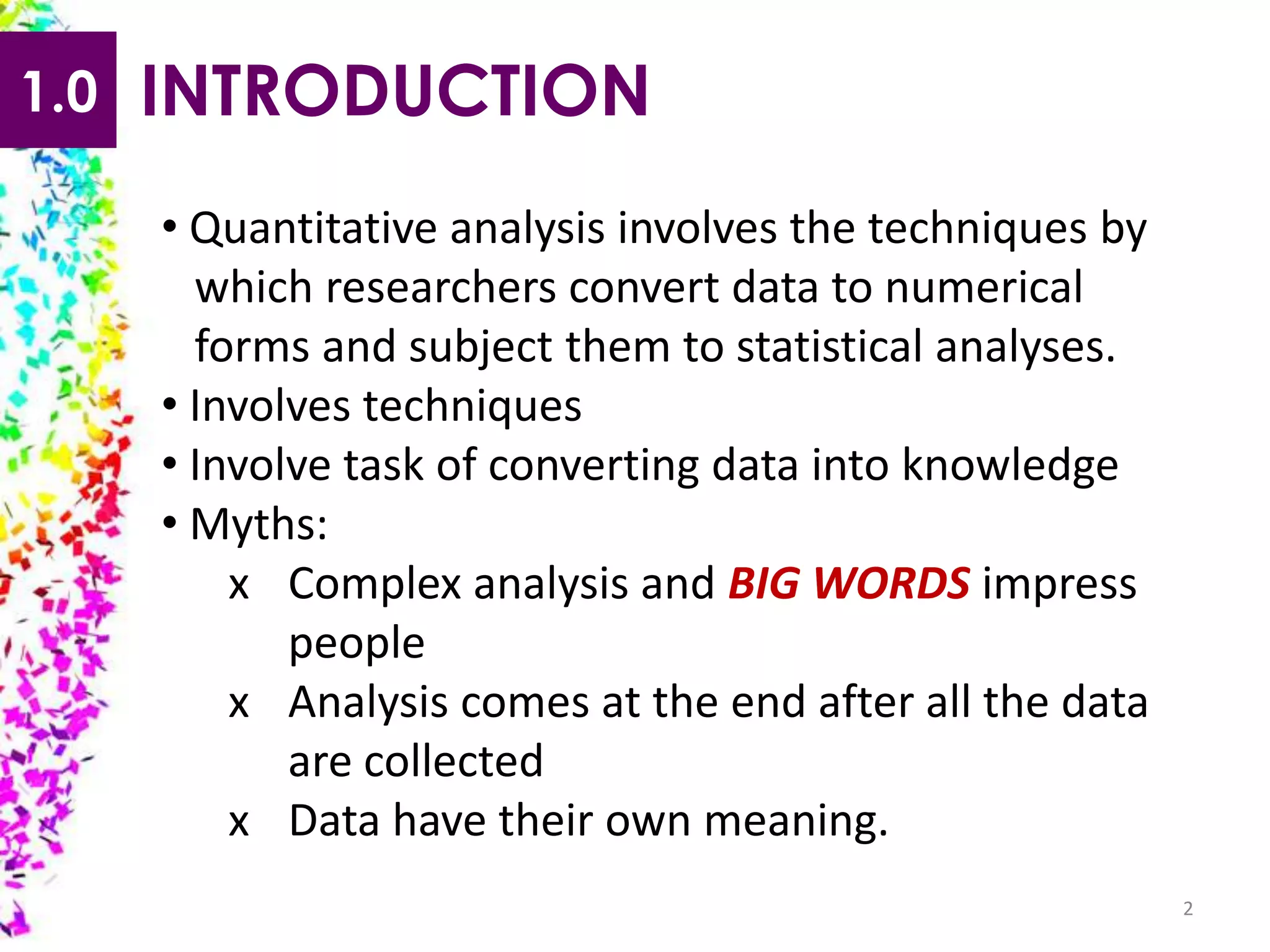
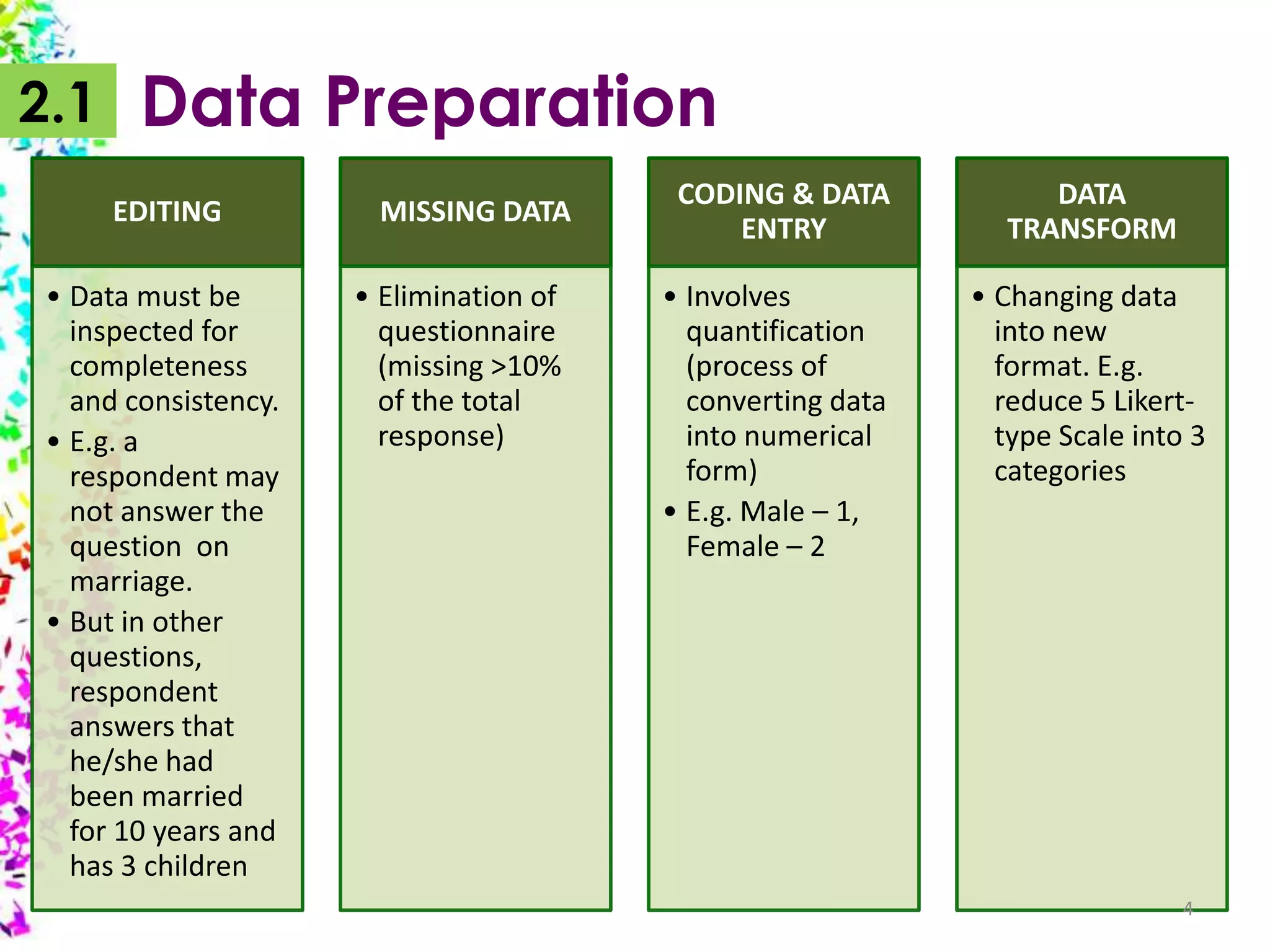
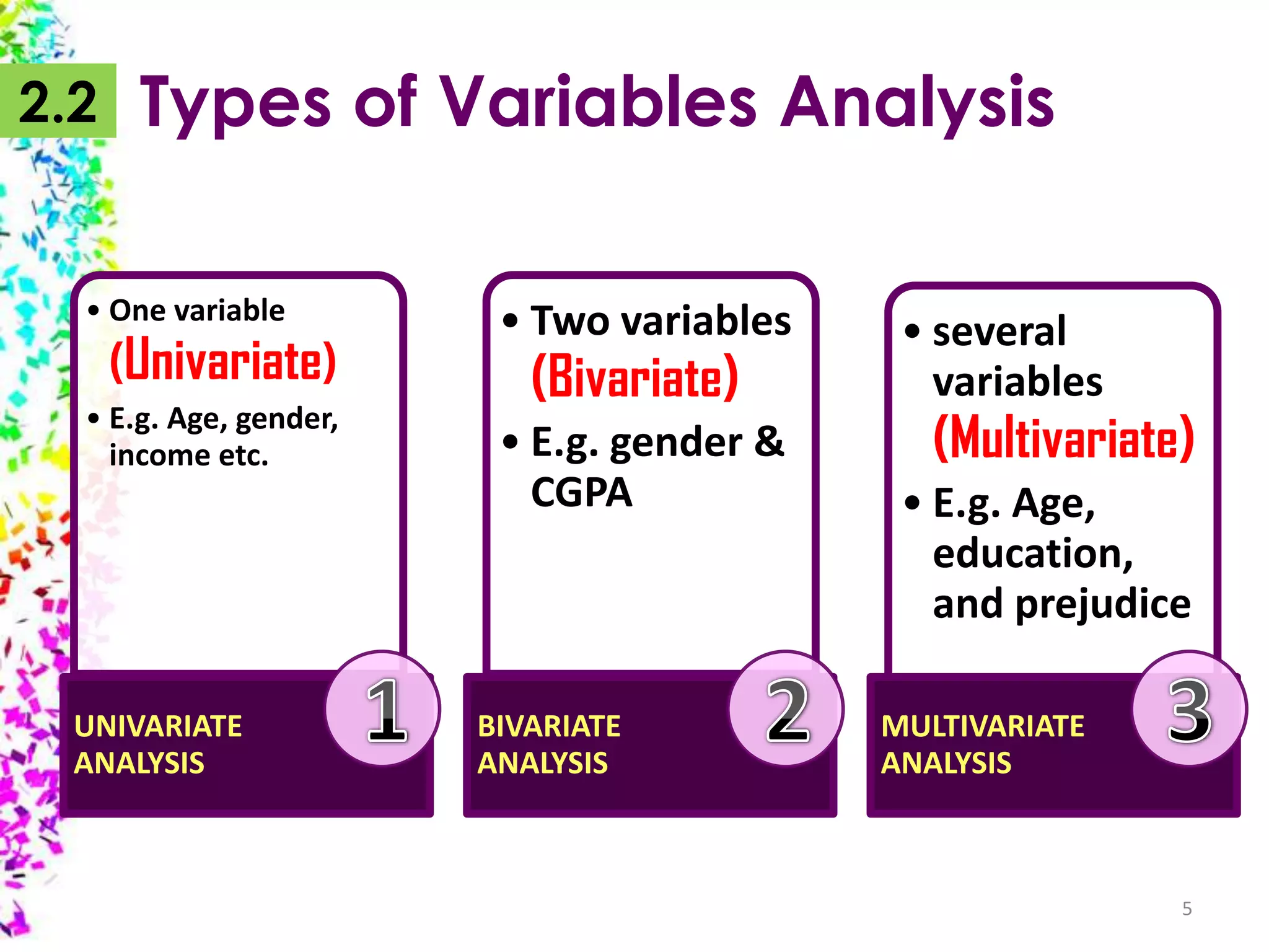
The document provides an overview of quantitative data analysis, detailing techniques for converting data into numerical forms and conducting statistical analyses. It covers the preparation, types of variables, univariate and bivariate analyses, along with subgroup comparisons and handling complex data. The conclusion emphasizes the significance of quantitative analysis in revealing genuine phenomena versus chance occurrences.

1. Quantitative
Data Analysis
Presenter:
ASMA MUHAMAD
FARHANA BINTI YAAKUB
1

2. 1.0
INTRODUCTION
• Quantitative analysis involves the techniques by
which researchers convert data to numerical
forms and subject them to statistical analyses.
• Involves techniques
• Involve task of converting data into knowledge
• Myths:
x Complex analysis and BIG WORDS impress
people
x Analysis comes at the end after all the data
are collected
x Data have their own meaning.
2

3. 2.0
QUANTIFICATION OF DATA
The numerical representation
and manipulation of
observations for the purpose
of describing and explaining
the phenomena that those
observation reflect.
(Babbie, 2010, p. 422)
3

4. 2.1
Data Preparation
EDITING
• Data must be
inspected for
completeness
and consistency.
• E.g. a
respondent may
not answer the
question on
marriage.
• But in other
questions,
respondent
answers that
he/she had
been married
for 10 years and
has 3 children
MISSING DATA
• Elimination of
questionnaire
(missing >10%
of the total
response)
CODING & DATA
ENTRY
• Involves
quantification
(process of
converting data
into numerical
form)
• E.g. Male – 1,
Female – 2
DATA
TRANSFORM
• Changing data
into new
format. E.g.
reduce 5 Likerttype Scale into 3
categories
4

5. 2.2
Types of Variables Analysis
• One variable
(Univariate)
• E.g. Age, gender,
income etc.
UNIVARIATE
ANALYSIS
• Two variables
(Bivariate)
• E.g. gender &
CGPA
BIVARIATE
ANALYSIS
• several
variables
(Multivariate)
• E.g. Age,
education,
and prejudice
MULTIVARIATE
ANALYSIS
5

6. 3.0
UNIVARIATE ANALYSIS
Univariate analysis is the
analysis of a single
variable.
Because Univariate
Analysis does not involve
relationships between
two or more variables, its
purpose is more toward
descriptive rather than
explanatory.
6

7. 3.1
Distribution
Frequency distribution is counts of the number of
response to a question or to the occurrence of a
phenomenon of interest.
(Polonsky & Waller, 2011, p. 189)
Obtained for all the personal data or classification
variables.
(Babbie, 2010, p. 428)
Gives researcher some general picture about the
dispersion, as well as maximum and minimum
response.
7

8. Distribution (cont’)
1.
What is your religious preference?
__1 Protestant __2 Catholic __3 Jewish ___4 None __5 Other
TABLE 3.1: Religious Preferences
Frequency
1 Protestant
2 Catholic
3 Jewish
4 None
5 Other
Total
Missing 9 NA
Total
Percent
886
367
26
146
52
1477
9
1486
59.6
24.7
1.7
9.8
3.5
99.4
0.6
100.0
Valid
Percent
60.0
24.8
1.8
9.9
3.5
100.0
Cumulative
Percent
60.0
84.8
86.6
96.5
100.0
Gusukuma, 2012. University of Mary Hardin-Baylor
8

9. Distribution (cont’)
FIGURE 3.2: Religious Preferences
Missing
6%
Other
3%
None
Jewish
9%
2%
Catholic
23%
Protestant
57%
9

10. 3.2
Central Tendency
Present data in form of an average:
1. Mean =
2. Mode = most frequently occurring attribute
3. Median = Middle attribute in the ranked distribution of
observed attribute
10

11. Central Tendency (cont’)
1
2
3
4
5
6
7
8
9
10
11
12
13
Age
20
19
20
20
19
18
19
17
18
18
19
21
23
251
GPA
1.9
1.5
2.1
2.4
2.75
3
2.85
2.75
3.3
3.1
3.4
4
3.9
36.95
Mean
19.308
2.8423
4.5385
Variance
Std Dev
2.3974
1.5484
0.5437
0.7374
5.6026
2.367
19
2.85
5
Dick
Edward
Emmett
Lauren
Mike
Benjie
Joe
Larry
Rose
Bob
Kate
Sally
Sylvia
Sum
Median
Gender
M
M
M
F
M
M
M
M
F
M
F
F
F
Hours
1
1
2
3
4
4
5
5
5
6
7
8
8
59
AGE OF RESPONDENTS
Mean = Sum
N
= 251
13
Mode = Most frequent
value
= age 19 (4)
Median = 19
11

12. 3.3
Dispersion
• Distribution of values around some central value, such
an average.
• Example measure of dispersion:
Range:
The distance separating the highest from the lowest value.
Variance
To describe the variability of the distribution.
Standard deviation:
An index of the amount of variability in a set of data.
Higher SD means data are more dispersed.
Lower SD means that they are more bunched together.
12

13. 3.4 Continuous & Discrete Variables
Continuous Variable
• A variable can take on any value between two specified values.
• An infinite number of values.
• Also known as quantitative variable
E.g. Income & age
Scale: Interval & Ratio
Discrete Variable
• A variable whose attribute are separate from one another.
• Also known as qualitative variable
E.g. Marital status, gender & nationality.
Scale: Nominal & Ordinal
13

14. 4.0
SUBGROUP COMPARISON
Bivariate and multivariate analyses aimed primarily at
explanation.
Before turning into explanation, we should consider the case
of subgroup description.
TABLE 4.1: Marijuana Legalization by Age of Respondents, 2004
Under 21
Should be legalized
Should not be legalized
100%=
21-35
36-54
55 & older
27%
40%
37%
24%
73
60
63
76
(34)
(238)
(338)
(265)
Source: General Social Survey, 2004, National Opinion Research Center.
Subgroup comparisons tell how different groups responded
to this question and some pattern in the results.
14

15. 4.1 “Collapsing” Response Categories
Combining the two appropriate range of variation to get
better picture or meaningful analyses.
TABLE 4.2: Attitudes toward the United
Nations. “ How is the UN doing in solving the
problems it has had to face?
TABLE 4.3: Collapsing Extreme Categories
Source. “5-Nation Survey Finds Hope for
U.N., New York Times, June 26, 1985, p.6
15

16. 4.2 Handling “Don’t Knows”
Whether to include or exclude the ‘don’t knows’ is harder to
decide.
TABLE 4.3: Collapsing Extreme Categories
TABLE 4.4: Omitting the “Don’t Knows”
EXCLUDED
 Different / Meaningful interpretation can be made.
 But sometimes the “Don’t Knows” is important.
 It’s appropriate to report your data in both forms –
so your readers can draw their own conclusion.
16

17. 4.3 Numerical Descriptions in Qualitative Research
The discussions are also relevant to qualitative studies.
The findings off in-depth, qualitative studies often can be
verified by some numerical testing.
EXAMPLE:
David Silverman wanted to compare the cancer treatments received by
patients in private clinics with those in Britain’s National Health Service.
He primarily chose in-depth analyses of the interactions between
doctor & patients.
He also constructed a coding form which enabled him to collate a
number of crude measures of doctor & patients interactions.
< Average = 10 to 20 minutes; Average = 21 to 30 minutes; > average =
more than 30 minutes
17

18. 5.0
BIVARIATE ANALYSIS
 In contrast to univariate analysis, subgroup
comparisons involve two variables.
 Subgroup comparisons constitute a kind of
bivariate analysis – the analysis of two variables
simultaneously.
 However, as with univariate analysis, the purpose
of subgroup comparisons is largely descriptive.
 Most bivariate analysis in social research adds on
another element: determining relationships
between the variables themselves.
18

19. BIVARIATE ANALYSIS
TABLE 5.1: Religious Attendance Reported by Men and Women in 2004
 Table describes the church attendance of men & women as
reported in 1990 General Social Survey.
 It shows: comparatively & descriptively – that women in
the study attended church more often as compared to men.
 However, the existence of explanatory bivariate analysis tells
a somewhat different story. It suggests: gender has an effect
on the church attendance.
19

20. BIVARIATE ANALYSIS
Theoretical interpretation of Table 1 in this
subtopic might be taken from CHARLES
GLOCK’S COMFORT HYPOTHESIS:
1. Women are still treated as secondclass citizens in U.S. society
2. People denied status gratification
in the secular society may turn to
religion as an alternative source of
status.
3. Hence, women should be more
religious than men.
20

21. 5.1 Percentaging a Table
In reading a table that someone
else constructed, one needs to
find out which direction it has
been percentaged.
Figure 5.1 reviews the logic by
which we create percentage
tables from two variables.
Variables gender and attitudes
toward equality for men and
women is used.
21

22. Percentaging a Table (cont’)
Figure 5.1: Percentaging a Table
a. Some men and women who either favor (+) gender equality
or don’t (-) favor it.
b. Separate the men from the women (the independent variable).
22

23. Percentaging a Table (cont’)
c. Within each gender group, separate those who favor equality from
those who don’t (the independent variable)
d. Count the numbers in each cell of the table.
23

24. Percentaging a Table (cont’)
e. What percentage of the women favor equality?
f. What percentage of the men favor equality?
24

25. Percentaging a Table (cont’)
g. Conclusion
TABLE 5.2: Gender and attitudes toward
equality for men and women.
RULES TO READ TABLE:
1. If the table percentaged
DOWN, read ACROSS.
2. If the table percentaged
ACROSS, read DOWN.
While majority of both men and women favored gender
equality, women are more likely than men to do so.
Thus, gender appears to be done of the causes of attitudes
toward sexual equality.
25

26. 5.2 Constructing and Reading Bivariate Tables
Steps involved in constructing of explanatory bivariate tables
1. The cases are divided into groups
according to attributes of the TABLE 5.2: Gender and attitudes toward
independent variable.
equality for men and women.
2. Each of these subgroups is then
described in terms of attributes of the
independent variable.
3. Finally, the table is read by comparing
the independent variable subgroups
with one another in terms of a given
attribute of the dependent variable.
26

27. 6.0
MULTIVARIATE ANALYSIS
The analysis of the simultaneous relationships among
several variables.
E.g. The effects of Religious Attendance, Gender, and Age
would be and example of multivariate analysis.
TABLE 6.1:
Multivariate Relationship: Religious Attendance, gender, and Age
Age
Gender
Religious
Attendance
Source: General Social Survey, 1972 – 2006, National Opinion Research Center.
27

28. 7.0
SOCIOLOGICAL DIAGNOSTICS
Sociological diagnostics is a quantitative analysis technique
for determining the nature of social problems such as
ethnic or gender discrimination.
(Babbie, 2010, p. 446)
It can be used to replace opinions with facts and to settle
debates with data analysis.
EXAMPLE:
Issues of GENDER and INCOME
Because family pattern, women as group have
participated less in in the labor force and many only begin
outside the home after completing certain child-rearing
tasks.
28

29. 8.0
CONCLUSION
In quantitative data analysis we classify features, count
them, and even construct more complex statistical models
in an attempt to explain what is observed.
Findings can be generalized to a larger population, and
direct comparisons can be made between two corpora, so
long as valid sampling and significance techniques have
been used.
Thus, quantitative analysis allows us to discover which
phenomena are likely to be genuine reflections of the
behavior of a language or variety, and which are merely
chance occurrences.
29

30. REFERENCES
Assessment Committee. (2009). Quantitative Data Analysis.
Unpublished PowerPoint Presentation. Emory University.
Babbie, E. (2010). The Practice of Social Research (Twelfth
ed.). California: Wadsworth Cengage Learning.
Gusukuma, I. V. (2012). Basic Data Analysis Guidelines for
Research Students. University of Mary Hardin-Baylor.
Hair, Jr., J. F., Money, A. H., Samouel, P., & Page, M. (2007).
Research Methods for Business. England: John Wiley &
Sons Ltd.
30