SlideShare a Scribd company logo
1 of 61
Download to read offline
Student Name and Number___________________________________________ Page 1 of 61
The University of Lahore
Department of Technology (Civil Division)
Lab Manual
of
Engineering Hydrology (CE-332)
Name: Roll No :
Section:
Student Name and Number___________________________________________ Page 2 of 61
Sr No. Design No. Page
01
To plot a graph for the given data of temperature (T) and saturated vapor
pressure (es) of air showing that the saturated vapor pressure is a function of
the temperature. Also find the following for the given conditions
04
02 Annual precipitation at rain gauge ‘X’ and the average annual precipitation at -
------ surrounding rain gauges are listed in the following table
12
03
The names, locations by latitude and longitude and mean annual precipitations
for certain weather stations
23
04
Given below are data for a station rating curve. Extend the relation and
estimate the flow at a stage of (------m) by logarithmic and Chezy’s methods
32
05
Following are the ordinates of a storm hydrograph for a river draining
catchments area of ----------- km2 due to a ---------- hours isolated storm. Drive
the ordinates of --------- hour’s unit hydrograph for the catchment.
39
06
The ordinates of a ------- hrs unit hydrograph are given below. Derive the
ordinates of:
S-curve hydrograph
45
07
The thickness of a horizontal, confined, homogeneous isotropic aquifer of
infinite areal extent is ------ m. A well fully penetrating the aquifer was
continuously pumped at a constant rate of ------ m3/sec for a period of 1 day.
The drawdown given in the table were observed in a fully penetrating well -----
- m from the pumping well. Compute the transmissivity (T) and storativity (S)
by using Thiess method.
51
Student Name and Number___________________________________________ Page 3 of 61
Preface
This design manual is intended to provide undergraduate engineering students an understanding
of the basic principles of engineering hydrology. It covers all designs related to the subject of the
level of 3rd
year B.Sc. Civil Engineering.
In this text, related theory is designed with the help of photographs of equipment to quickly
grasp the basic concepts. To further elaborate the theory blank spaces are provided to draw some
sketches related to the design. It also contains brief procedure for undertaking designs, self-
explanatory tables for calculations, blank graph sheets to plot graphs, blank spaces for writing
results and finally comments on the results. As practiced universally, SI units are used in this
manual. However, wherever felt necessary, values in alternate units re also provided to facilitate
students.
In this design manual, totally six designs are provided covering various topics of the field of
hydrology.
Design No. 1, 2 and 3 are related to precipitation.
Design No. 4 covers the topic “extension of rating curve” for a stream gauging station.
Design No. 5 and 6 help in understanding the theory of hydrographs.
Any comments / suggestions by the teachers / students will be highly appreciated.
Student Name and Number___________________________________________ Page 4 of 61
Design No. 1
To plot a graph for the given data of temperature (T) and saturated vapor pressure (es) of
air showing that the saturated vapor pressure is a function of the temperature. Also find
the following for the given conditions
Saturation Deficit (es – e)
Relative Humidity (f)
Dew point temperature (Td)
Condition No.
Air Temperature (T)
(°C)
Vapor Pressure (e)
(mm of Hg)
1
2
3
4
Related Theory
Hydrology
It is the scientific study of hydrological cycle. Schematic diagram showing the hydrological
cycle is presented in Figure 1.1.
Figure 1.1: Pictorial view showing the global hydrological cycle.
Student Name and Number___________________________________________ Page 5 of 61
Hydrology is the science of waters of the earth, their circulation and distribution over the globe,
their physical and chemical properties and their interaction with the physical and biological
environment (Aswan N. M. 1981).
Hydrology is concerned with the circulation of water and its constituents through the hydrologic
cycle. It deals with precipitation, evaporation, infiltration, groundwater flow, runoff, stream flow
and the transport of substances dissolved or suspended in flowing water. Hydrology is primarily
concerned with water on or near the land surface; ocean waters are the domain of oceanography
and the marine sciences (Maidment 1993).
Hydrology is an earth science. It encompasses the occurrence, distribution, movement, and
properties of the waters of the earth. Knowledge of hydrology is fundamental to decision making
process where water is a component of the system of concern. Water and environmental issues
are inextricably linked, and it is important to clearly understand how water is affected by and
how water affects ecosystem manipulations (Viessman Warren 1996).
Engineering Hydrology
Engineering hydrology includes those segments of the field pertinent to planning, design and
operation of engineering projects for the control and use of water (Linsley 1982).
Significance of Hydrology
Study of water is extremely necessary as:
I. It is the basic need for the sustenance of human life over the planet (drinking, agriculture
and industry).
II. To cope with the extreme hydrological events (floods and droughts).
III. To determine input data for the design of hydraulic structures (Design floods and
sediment inflows).
Meteorology
It is the science of atmosphere which is gaseous envelope surrounding the earth (Awan N. M.
1981).
Student Name and Number___________________________________________ Page 6 of 61
Climatic Factors
Meteorology of the region is affected by certain climatic factors.
I. Amount and distribution of precipitation.
II. The occurrence of snow and ice.
III. Wind velocity.
IV. Temperature.
V. Humidity.
Importance of Knowledge of Meteorology
I. Cloud formation.
II. Occurrence of precipitation.
III. Thunder storm formation.
IV. Movement of rainstorms.
V. Weather forecast.
VI. As the meteorological phenomena are the forerunners of floods, flood warnings and
forecasts may be issued in advance if one can make use of the meteorological conditions
that are likely to produce floods. Knowledge of meteorology is also essential prerequisite
in the understanding of evaporation phenomenon.
Atmosphere
Atmosphere is the gaseous envelop around the earth surface. It consists of many gases like N2,
O2, CO2 etc and water vapours. The term is derived from the Greek work atoms (vapor of
breath) and sphaira (sphere or ball) (Aswan N. M. 1981).
Troposphere / Hydrosphere
It is the layer of atmosphere adjacent to the surface of the earth, which contains about 99% of
total atmospheric water. Its average thickness is about 12 km. For civil engineers this is the most
important atmospheric layer. All processes like cloud formation, thunderstorms, and
precipitation take place in this layer.
Student Name and Number___________________________________________ Page 7 of 61
Figure 1.2: Photograph showing layers of atmosphere and their average thicknesses.
Atmospheric Water
It is the water available in the atmosphere (troposphere / hydrosphere), in the form of water
vapors’, ice crystals, clouds and precipitating particles etc. The quantity of water in atmosphere
is approximately 12.900 Km3
, which is about 0.001% of total global water and 0.5% of volume
of the atmosphere (Chow 1988).
Vaporization
It is the process of transformation of water from liquid state to vapor state. The process of
vaporization at global scale is shown in Figure 1.3.
Figure 1.3: Conceptual diagram showing the phenomenon of evaporation.
Vapor Pressure (e)
Pressure exerted by the water vapors in air is known as vapors in air is known as paver pressure.
Its commonly used units are mm of Hg.
Student Name and Number___________________________________________ Page 8 of 61
Graph showing relationship between air temperature and saturation vapor pressure.
Saturation Vapor Pressure (es)
It is the vapor pressure when air is fully saturated at a given temperature. It is the measure of
moisture holding capacity of air, which increases with increase in air temperature as shown in
Figure 1.4.
Sr. #
Air Temperature
(°C)
Saturated Vapor Pressure
(mm of Hg)
1
2
3
4
5
6
7
8
9
10
11
12
13
14
15
16
17
18
19
20
Student Name and Number___________________________________________ Page 9 of 61
Saturation Deficit
The difference between the saturation vapor pressure and vapor pressure of the air at a given
temperature is called saturation deficit.
∆ e = es - e (1.1)
Where ∆ e is saturation deficit, es is the saturation vapor pressure and e is the vapor pressure.
Humidity
It is the presence of moisture in the air. Humidity in the atmosphere can be assessed by vapor
pressure of air.
Relative Humidity
It is the ratio between the vapor pressure and the saturation vapour pressure of air at a given
temperature. It is usually expressed in percentage.
f =
𝒆
𝒆𝒔
x 100 (1.2)
Dew Point Temperature (Td)
The dew point temperature can be defined as the temperature at which the air mass just becomes
saturated if cooled at constant pressure with moisture neither added nor removed (Awan N. M.
1981).
Once air is cooled naturally to this temperature dewdrops are formed. This usually happens at
late night when temperature falls significantly.
Student Name and Number___________________________________________ Page 10 of 61
Table 1.2: Table of Calculations:-
Sr. #
Air
Temperature
(°C)
Vapor
Pressure (e)
(mm O Hg)
Saturated
Vapor
Pressure
(es)
(mm of Hg)
Saturation
Deficit
(es – e)
(mm of Hg)
Relative Humidity
e
f = --------- x 100
es
(%)
Dew Point
Temperature
(Td)
(°C)
1
2
3
4
Procedure
1. Plot a graph between saturated vapor pressure (es) and air temperature (T) choosing
suitable scale.
2. Plot condition 1 for a given e & T on es ~ T graph.
3. For point 1, draw a vertical line passing through the point up to the saturation line,
measure distance between saturation line; it is the saturation vapor pressure for point 1.
4. Measure vertical distance between point 1 and saturated line, it is saturation deficit.
5. Compute relative humidity by using equation (1.2).
6. Draw a horizontal line from point 1 to the left, it may intersect with the saturation curve.
Note down the temperature for the intersection point, it is the dew point temperature.
7. Repeat steps 2 to 6 for points 2, 3 and 4.
Results
The results of the design exercise are presented in the last three columns of Table 1.2.
Student Name and Number___________________________________________ Page 11 of 61
Comments
Student Name and Number___________________________________________ Page 12 of 61
Design No. 2
Annual precipitation at rain gauge ‘X’ and the average annual precipitation at -------
surrounding rain gauges are listed in the following table
Examine the consistency of station ‘X’ data.
When did the change in the regime occurred? Discuss possible reasons.
Adjust the data and determine what difference this makes to the -------- years annual
precipitation at station ‘X’.
Table 2.1: Observations
Year
Average Annual PPT. (cm).
Station ‘X’
Average of ------- Surrounding
Stations
Student Name and Number___________________________________________ Page 13 of 61
Related Theory
Precipitation
All types of moistures reaching to the surface of earth from atmosphere is known as
precipitation. The precipitation on land surface is about one 3rd
of the total global precipitation.
The precipitation on land surface is due to 10% evaporation from land and 90% evaporation
from oceans (Chow 1988).
Figure 2.1: Climatological station showing various equipment.
Forms of Precipitation
At a place, precipitation may fall in one or more than one following forms.
i. Drizzle or Mist
ii. Rain
iii. Snow
iv. Sleet
v. Glaze
vi. Hail
vii. Fogs
viii. Frost
ix. Trace
Student Name and Number___________________________________________ Page 14 of 61
Drizzle or Mist
It is the precipitation in the form of tiny liquid droplets having diameter from 0.1 mm to 0.5 mm.
Its intensity rarely increases 1 mm / hr (Linsley 1982).
Rain
Precipitation in the form of liquid droplets of diameters ranges from 0.5 mm to 6 mm. Its
intensity is greater than 1mm /hr. According of U.S.A metrological department rainfall is
classified as:
a. Light Rain I< 2.5 mm / hr
b. Moderate Rain 2.5 mm / hr < I < 7.6 mm / hr
c. Heavy Rain I > 7.6 mm / hr
Figure 2.2: Standard rain gauge at a Climatological station.
Snow
It is the precipitation in the form of ice crystals. Specific gravity of fresh fallen snow is
approximately 0.1.
Sleet
It is precipitation in the form of mixture of liquid drops and ice crystals.
Student Name and Number___________________________________________ Page 15 of 61
Glaze
It is the ice coating generally clear and smooth on exposed surfaces by the freezing of super
cooled water deposited by the rain.
Hails
It is the precipitation in the form of ice balls or lumps. Diameter of hail ranges from 5 mm to 125
mm (Linsley 1982).
Figure 2.3: Weather station for the measurement of precipitation, wind speed, wind direction and
minimum and maximum temperatures.
Fog
It is the precipitation in the form of weak cloud clone reaching to the surface of earth. Due to
very small size droplets it remains suspended in air for some time. Fog produces a lot a visibility
problem.
Frost
It is the precipitation in the form of frozen dewdrops on the land surface.
Trace
It is the very small amount precipitation at a remain gauging station, usually less than or equal to
0.125 mm.
Student Name and Number___________________________________________ Page 16 of 61
Mechanism To From Precipitation
There are four mechanisms necessarily required for the occurrence of precipitation over an area.
Lifting Mechanism
Water vapor is present in air even in cloudless days. There are three mechanisms available in
nature for lifting moisture-laden air to higher levels where condensation is possible due to having
very low air temperatures.
a. Convective systems
b. Orographic barriers
c. Cyclones
Formation of Cloud Droplets / Ice Crystals
Condensation of water vapor into cloud droplets takes place on hygroscopic nuclei or
condensation nuclei. These are tiny particles having affinity for water. The sources of these
condensation nuclei are the particles of sea salt and products of sulsphurus and nitrous acids
(Linsley 1982).
Condensation will occur if air in atmosphere is cooled to saturation. Condensation nuclei range
in size from 0.1 μ m to 10 μ m.
For the formation of ice crystals, freezing nuclei are required which usually consist of clay
minerals (Kaolin).
Growth of Cloud Droplets / Ice Crystals
Cloud elements are generally smaller than 50 μ m in diameter. The droplet size must be large
enough for the occurrence of precipitation to overcome the buoyant force and drag force
produced due to vertical relative motion between cloud droplet and air. Moreover, cloud
elements must also be large enough to penetrate the unsaturated air below the cloud base without
evaporating completely.
An upward current of less than 0.5 cm / s is sufficient to keep from falling to precipitating
droplets have diameters under 10 μ m. Ice crystals of the same weight (larger size) can be
Student Name and Number___________________________________________ Page 17 of 61
supported by even lesser velocities. In nature, there are two processes available for the growth of
cloud elements.
a. Coalescence of Cloud Droplets
This is the growth of cloud droplets due to collision of larger drops with smaller one. At an
average, 7 collisions take place per km fall of droplet.
b. Coexistence of Ice Crystals and Cloud Droplets
If in a layer of clouds there is moisture of water droplets and ice crystals, the saturation vapor
pressure over ice is lower than over water. As a consequence of this difference there results
evaporation of water drops and condensation of much of this water on ice crystals causing
their growth and ultimate fall through the clouds. This effect is known as Bergeron’s effect.
The ice crystals will further grow as they fall and collide with water droplets.
Sufficient Accumulation of Moisture over an Area
For the occurrence of heavy precipitation over an area requires heavy water vapor presence in
the atmosphere. It needs a large net horizontal inflow of water vapor into the atmosphere above
the basin area. This process is called convergence.
Rain Gauge
It is an instrument used to measure the amount of rainfall or intensity of rainfall at a place. A
typical Climatological station is shown in Figure 2.1, a standard rain gauge in Figure 2.2 and a
weather station in Figure 2.3 which can measure precipitation, wind speed, wind direction,
minimum and maximum temperatures.
Amount of Precipitation (mm or inches)
It is total depth of rainfall over an area usually in one day.
Student Name and Number___________________________________________ Page 18 of 61
Intensity of Precipitation
Reference: It is the amount of precipitation at a place per unit time (rain rate). It is usually
expressed in mm / hr.
Mean / Average Rainfall for N Years
It the arithmetic average of annual precipitations for N years over a rain gauging station.
Mathematically:
(2.1)
Where Pavg is the average precipitation, N is the total number of years and Pi is the annual
precipitation for ith
year.
Annual Rainfall
Total amount of rainfall accumulated in one year at a place, mathematically it is expressed as:
(2.2)
Where,
Pann is he annual precipitation at a rain gauging station and Pi is the daily precipitation.
Average Rainfall over an Area
It is amount of precipitation which can be assumed as uniform for the area. It is estimated by
using several approaches. One is the arithmetic mean as defined mathematically:
(2.3)
Student Name and Number___________________________________________ Page 19 of 61
Where,
Pavg is the areal average precipitation, N is the total number of stations and Pi is the average
annual precipitation for it h station.
Reasons of Inconsistency in Precipitation Data Record
a. Change in Location of a rain gauge.
b. Change of instrument (rain gauge).
c. Change in observational procedures.
Procedure
1. Calculate cumulative annual precipitation for station ‘X’.
2. Calculate cumulative average annual precipitation of ‘N’ surrounding stations.
3. Plot scatter diagram between cumulative annual precipitation of station ‘X’ and
cumulative average annual precipitation of ‘N’ surrounding stations.
4. Joint points carefully with straight lines and note down the intersection point.
5. Determine slopes of the two curves.
6. Compute ratio
S1
S2
7. Adjust average annual precipitation of station ‘X’ after the change has occurred.
Figure 2.4: Locations of station ‘X’ and surrounding stations in a basin.
Student Name and Number___________________________________________ Page 20 of 61
Table 2.1: Computations for Double Mass Analysis
Year
Annual Precipitation (cm)
Cumulative
Annual Precipitation (cm)
Adjusted
Annual
PPT at
Station ‘X’
(cm)
Station ‘X’
Average of
20
Surrounding
Stations
Station ‘X’
Average of
20
Surrounding
Stations
Col 1 Col 2 Col 3 Col 4 Col 5
Student Name and Number___________________________________________ Page 21 of 61
Results
Student Name and Number___________________________________________ Page 22 of 61
Comments
Student Name and Number___________________________________________ Page 23 of 61
Design No. 3
The names, locations by latitude and longitude and mean annual precipitations for certain
weather stations within and outside the catchment’s area are given below:
Name of Stations Latitude
(____º____)
Longitude (
º____)
Mean Annual PPT.
(cm)
Estimate he average rainfall over the basin area by using following three methods.
i. Arithmetic Mean Method
ii. Thiessen Polygon Method
iii. Isohyetal Method
The boundary of the watershed is rectangular and is defined by following four coordinates:
A ( )
B ( )
C ( )
D ( )
Student Name and Number___________________________________________ Page 24 of 61
Related Theory
Average Precipitation over an Area
It is the amount of precipitation which can be assumed uniform for the entire area. By simplest
method, it can be obtained by adding the precipitations of all stations and dividing by the number
of stations in the area or outside the area closer to the boundary. The rain gauges used to measure
precipitation are shown in Figure 3.1.
Significance of Average Precipitation
If average precipitation over an area is known, then it is very easy to compute the total volume of
rainfall received by the area for nature. Rainfall volume = Area x Average precipitation.
Student Name and Number___________________________________________ Page 25 of 61
Figure 3.1 Showing Rain Guages
Figure 3.3 showing Isohyetal Method
Figure 3.2 showing Thiessen Polygon Method
Student Name and Number___________________________________________ Page 26 of 61
Methods of Finding Average Precipitation over an Area
There are three common methods for averaging precipitation over an area.
i. Arithmetic Mean Method
ii. Thiessen Polygon Method
iii. Isohyetal Method
Arithmetic Mean Method
It is the simplest method of averaging precipitation over an area. This method is applicable
where precipitation gauging stations are more or less equally spaced and also precipitation
amounts do not vary significantly with each other.
The average precipitation over an area by arithmetic mean method is obtained as follows:
(3.1)
Where N is total number of stations and P1 is mean annual precipitation at ith station.
Table 3.1: Average Precipitation by Arithmetic Mean Method:-
No. of Stations Name of Stations Mean Annual PPT. (cm)
Student Name and Number___________________________________________ Page 27 of 61
Thiessen Polygon Method
The fundamental principle followed in this method consists of weighing the value of
precipitation at each station by a suitable proportion of basin area. Therefore ppt. data is plotted
over a map (graph). The Thiessen polygon map for a typical watershed is shown in Figure 3.2.
Procedure
1. Select suitable and same scale for X and Y-axis.
2. Plot catchment’s boundary and station locations.
3. Plot polygons around each strength by connection closest station by straight dashed
lines and drawing perpendicular bisectors to make the sides of polygon.
4. Determine area of each polygon by counting the number of squares.
5. Compute product (P1 A1) and sum all products.
6. Compute average precipitation using following equation.
(3.2)
Where, N is number of polygons within catchments, P1 is the mean annual precipitation for ith
polygon and A1 is the area of ith polygon.
Student Name and Number___________________________________________ Page 28 of 61
Table 3.2: Table of calculations for Thiessen Polygon Method:-
Sr. # Gauging
Stations
Observed
Annual ppt.,
Pi (cm)
Area of
Polygon, Ai
(min2)
Product (Pi
Ai)
(mm min2)
Isohyetal Method
Isohyets
It is the line representing the same amount of precipitation. In Isohyetal method, area between
two consecutive isohyets is determined. Weighted average precipitation for each segment is
computed and then average precipitation for the entire basin is determined. The Isohyetal map
for a typical watershed is shown in Figure 3.3 and Isohyetal map for annual precipitation over
Pakistan is shown in Figure 3.1.
Student Name and Number___________________________________________ Page 29 of 61
Procedure
i. Select suitable and same scale for X and Y-axis.
ii. Plot catchment’s boundary and station locations.
iii. Mention precipitation amounts on each station.
iv. Select suitable contour interval and number of isohyets.
v. Draw isohyets by linear interpolation between stations.
vi. Determine area between two consecutive isohyets.
vii. Calculate product (Pi Ai).
viii. Compute average precipitation by formula.
(3.3)
Where, N is number of strips / segments, Pi is the mean precipitation for ith strip and Ai is the
area of ith strip.
Table 3.3: Table of Calculations For Isohyetal Method:-
Sr. # Isohyetal
Precipitation
(mm)
Mean ppt. (mm) Area of Strip
(min2)
(mm. min2)
Student Name and Number___________________________________________ Page 30 of 61
Result
The average annual precipitation for the watershed is:
Pavg = mm by using mean arithmetic method.
Pavg = mm by using Thiessen polygon method.
Pavg = mm by using Isohyetal method.
Student Name and Number___________________________________________ Page 31 of 61
Comments
Student Name and Number___________________________________________ Page 32 of 61
Design No. 4
Given below are data for a station rating curve. Extend the relation and estimate the flow
at a stage of (------m) by logarithmic and Chezy’s methods:
Sr. # Stage, H (m) Mean Depth, D
(m)
X-Sec Area A
(m2)
Discharge, Q
(m3/sec).
Student Name and Number___________________________________________ Page 33 of 61
Related Theory
Stage
Stage is the height of the water surface above an arbitrary datum. In Figure 4.1 stage (H) and
depth (d) are shown on a stream section.
Stage Gauge
The instrument used for measuring stage at a gauging station is called stage gauge. The staff
stage gauges at a stream gauging station are shown in Figure 4.2.
Types of Gauges
There are two main types of stage gauges, i.e. Non-recording stage gauges and recording gauges.
Non-recording stage gauges are those, which do not record the stage values automatically. The
examples are staff stage gauge, wire weigh gauge etc.
Figure 4.1: Conceptual diagram showing the measurement of stage in a stream.
Recording stage gauges keep the record of stages automatically for a particular duration of time
say one day. The example is the float type stage gauge.
Student Name and Number___________________________________________ Page 34 of 61
Figure 4.2: Staff stage gauges at a stream gauging station.
Rating Curve
It is a graphical relationship between stage and discharge at a stream gauging station as shown in
Figure 4.3.
Flow (cumics)
Figure 4.3: A typical rating curve for a stream gauging station. Significance of Rating Curve
Student Name and Number___________________________________________ Page 35 of 61
i. To get discharge value corresponding to any stage value.
ii. To determine stage values corresponding to various flows for the construction of
hydraulics structures.
Figure 4.4: Graphical procedure for the extension of rating curve using Logarithmic Method.
How a Rating Curve is established at a Site
It is plotted by taking simultaneous measurements of stage and discharge at different water levels
(stages) in the steam at a particular section. The cross sectional area of flow is divided in a
number of segments assigning that in a particular segment the velocity remains uniform in width.
Velocity of flow is measured in each segment with the help of current meter. Then discharge is
computed in each segment and total discharge is determined by integrating it for the entire cross
section.
Figure 4.5: Graphical procedure for the extension of rating curve using Chezy’s Method.
Student Name and Number___________________________________________ Page 36 of 61
Extension of Rating Curve
Rating curves are established by collecting and plotting past data of stages and discharges for a
particular section of the stream. A flood magnitude (for higher returned periods) is expected at
any time in future greater than the highest observed in the past and the available rating curve
becomes useless for this value of flood stage. Then extension of rating curve becomes essential
to determine the flood magnitude on a value of the stage higher than the observed.
Methods of Extension of Rating Curve
Usually, there are two approaches for the extension of rating curve.
a. The logarithmic method.
b. Chezy’s method.
The Logarithmic Method
This method is used if the cross section of the steam at the gauging station is of regular shape.
Log Q = Log K + n log (H – a)
Chezy’s Method
This method is based on Chezy’s equation.
Q = AC √ RS
If the friction is uniform and bed slope S is constant
Q = AC √ S √ R
R=
A
P
=
bD
b + 2D
≈D
Q = A (C√ S) √ D
Q = (C√ S) A √ D
Q oc A √ D
Where b is the bed width, D is the mean depth of the stream, R is the hydraulic radius, S is the
slope of the energy line and Q is the flow rate in the channel. As flow is proportional to the A
Student Name and Number___________________________________________ Page 37 of 61
√ D , hence the graphical relationship between them should definitely be an straight line, which
can be easily extended up to required stage value.
The graphical procedure required for the extension of rating curve by Chezy’s method is shown
in Figure 4.5.
Table 4.1: Table of Calculations For The Extension of Rating Curve.
Sr.# Stage
H (m)
Depth
D (m)
Area
A
(m3
)
Discharge
Q
(cumics)
A√ D
(m2.5
)
LogQ Log (H-a)
a= a= a=
Student Name and Number___________________________________________ Page 38 of 61
Results
i. Flood magnitude, Q at ------m stage by logarithmic method is --------- m3/ S.
ii. Flood magnitude, Q at ------m stage by Chezy’s method is -------------- m3/ S.
Comments
Student Name and Number___________________________________________ Page 39 of 61
Design No. 5
Following are the ordinates of a storm hydrograph for a river draining catchments area of
----------- km2 due to a ---------- hours isolated storm. Drive the ordinates of --------- hour’s
unit hydrograph for the catchment.
Time From Start (Hours) Discharge (m3 / sec)
Student Name and Number___________________________________________ Page 40 of 61
Related Theory
Hydrograph
It is the graphical representation of flow against time for a particular section of the stream /
river.. Variable kept on y-axis is flow or discharge while on x-axis it is time.
Parts of Hydrograph
Hydrograph comprises of the following four parts.
i. Ground water recession curve.
ii. Rising limb.
iii. Peak
iv. Recession curve or falling limb.
Components of a Hydrograph
i. Direct runoff (DRO)
ii. Base flow
Factors Affecting the Shape of Hydrograph
The main factors affecting the shape of hydrograph are basically two, the climatic factors and
second are the physiographical factors. Climatic factors include the amount of rainfall, intensity
and duration of rainfall, while physical characteristics of the watershed include the shape of the
basin, slope of the watershed, surface conditions of the catchment and soil types in the
watershed.
Hydrograph Separation
The hydrograph separation means splitting the hydrograph ordinates in two parts i.e. the base
flow and direct runoff (DRO) ordinates.
Methods of Separation of Hydrograph
Following are the methods used for the separation of hydrographs.
Student Name and Number___________________________________________ Page 41 of 61
1. Straight line method.
a. Horizontal straight line method
b. Inclined line method
2. Fixed base length method
3. Variable slope method
In horizontal straight line method a horizontal line is drawn from the point of rise. The area
below the line is base flow. This line is based on the assumption that a constant amount of base
flow is maintained during the storm runoff. It produces an extremely long time base for the
DRO.
In inclined line method, inclined line is obtained by joining two points, i.e. Where DRO enters
and where DRO ceases. DRO ceases after N days from the pack discharge and is obtained by the
following relationship.
N = K (A) 0.2
Where N is the time in days after which DRO ceases from the peak and depends on the basin
characteristics, A is the area of the watershed and K is the coefficient, its value is 1 for area A in
Ml2 and 0.8 for A in km2, respectively.
In fixed base length method, a line AB is drawn in the extension of groundwater recession curve
ending at peak of the hydrograph (B). Another line BC is drawn from point B to C where DRO
ceases at a distance of N days from the peak of hydrograph. The area of hydrograph above curve
ABC is DRO and below is base flow (Linsley 1982).
Unit Hydrograph
It is the direct runoff hydrograph with unit effective precipitation over the entire watershed.
Applications of Unit Hydrograph
A unit hydrograph is used for the prediction of flood peak and time to peak in the stream at a
particular section due to any amount of effective precipitation over the watershed.
Assumptions For the UGH
i Precipitation amount and intensity is uniform over the entire watershed.
ii. Precipitation intensity remains uniform though out the storm.
Student Name and Number___________________________________________ Page 42 of 61
iii. Base length of hydrograph DRO for a particular catchments resulting from a storm of a
given duration is approximately constant.
iv. Entire watershed is treated as a single unit.
Procedure
i. Plot hydrograph of given data.
ii. Separate base flow and DRO.
iii. Determine volume of DRO in km3 or cft.
iv. Determine volume of DRO in cm or inches (x) by dividing the volume with
watershed area.
v. Compute ordinates of UHG ordinates = ordinates of DRO / X.
vi. Plot unit hydrograph.
vii. Check area under the curve of UHG, it should be 1 cm or 1 inch depending on the
system of units used.
Equation?
Student Name and Number___________________________________________ Page 43 of 61
Table 5.1: Derivation of the ordinates of unit hydrograph:-
Time For Start
(Hours)
Discharge (m3
/ sec)
Base Flow (m3
/ sec)
DRO (m3 /
sec)
Ordinates of
Unit
Hydrograph
(DRO / x)
Check for area under UHG =?
The area under UHG in cm is = ?
Student Name and Number___________________________________________ Page 44 of 61
Results
Comments
Student Name and Number___________________________________________ Page 45 of 61
Design No. 6
The ordinates of a ------- hrs unit hydrograph are given below. Derive the ordinates of:
S-curve hydrograph
-------- hrs unit hydrograph
Time (hrs)
Ordinates of ------
hrs Unit
Hydrograph (m3 /s)
Time (hrs)
Ordinates of ------
hrs Unit
Hydrograph (m3 /s)
Student Name and Number___________________________________________ Page 46 of 61
Related Theory
General
Any unit hydrograph for a catchment is associated with definite duration of rainfall and hence
cannot be used for all durations. It is therefore necessary to derive unit hydrograph of various
durations.
For this purpose it is not essential to use the actual rainfall data and the flood hydrograph
because a short duration unit hydrograph can be converted into a long or vice versa by S-curve
method provided other durations are integral multiple of given duration. Thus for example S-
curve method can be used to develop 12 hours unit hydrograph from a 4 hr unit hydrograph. It is
also called as conversation of UGH duration.
S-Curve
The S-curve is a hydrograph of surface runoff, which result from an addition of an infinite series
of T hr unit hydrograph each lagged by T hours (i.e. equal to the duration of the stream) with
respect to the preceding one. The S-curve becomes consultant after a period equal to the base
length of the unit hydrograph used to derive it.
Methods For S-Curve Generation
Following methods can be used for the derivation of S-curve ordinates.
1. Offset method.
2. S-curve addition method.
Student Name and Number___________________________________________ Page 47 of 61
Table 6.1: Derivation of S-Curve Ordinates by Offset Method
Time
(hrs)
Ordinates
of ----- hrs
UHG (m3
/s)
Off Set
Ordinates
of S-Curve
(m3 /s)
1 2 3 4 5
Table 6.2: Derivation of S-Curve, --------- hrs UHG and ---------- hrs UHG Ordinates
Student Name and Number___________________________________________ Page 48 of 61
Time
(hrs)
Ordinate
s of -----
hrs
UHG
(m3 /s)
S-Curve
Addition
al (m3 /s)
Ordinate
s of S-
Curve
(m3 /s)
S-
Curve
Lagge
d by --
- hrs
(m3 /s)
Diff.
of col.
(4) &
col.
(5)
(m3
/s)
Ordinates
of ----- hrs
UHG (m3
/s)
S-
Curve
Lagged
by ---
hrs
(m3 /s)
Diff. of
col. (4)
& col.
(8) (m3
/s)
Ordin
ates
of ----
- hrs
UHG
(m3
/s)
Col.(1) Col.(2) Col.(3) Col.(4) Col.(5) Col.(6) Col.(7) Col.(8) Col.(9) Col.(1
0)
Student Name and Number___________________________________________ Page 49 of 61
Procedure
Student Name and Number___________________________________________ Page 50 of 61
Results
Comments
Student Name and Number___________________________________________ Page 51 of 61
Design No. 7
The thickness of a horizontal, confined, homogeneous isotropic aquifer of infinite areal
extent is ------ m. A well fully penetrating the aquifer was continuously pumped at a
constant rate of ------ m3/sec for a period of 1 day. The drawdown given in the table were
observed in a fully penetrating well ------ m from the pumping well. Compute the
transmissivity (T) and storativity (S) by using Thiess method.
Time (min) Drawdown (m) Time (min) Drawdown (m)
Student Name and Number___________________________________________ Page 52 of 61
Related Theory
Aquifer
An aquifer is a water-bearing stratum or formation capable of transmitting water in quantities
sufficient to permit development. Aquifers may be considered as falling into two categories,
confined and unconfined, depending on whether a water table or free surface exists under
atmospheric pressure. Storage volume within an aquifer is changed whenever water is recharged
to, or discharged from, an aquifer (Viessman 1996).
Unconfined Aquifer
The top most water bearing strata having no confining impermeable overburden is known as
unconfined aquifer. This aquifer is also known as non-artesian aquifer or water table aquifer.
A special case of unconfined aquifer involves perched water bodies. This occurs whereas a
ground water body is separated from main water table by relatively impermeable stratum as
shown in Figure 7.1.
Figure 7.1: Schematic diagram showing the perched water table.
Student Name and Number___________________________________________ Page 53 of 61
Confined Aquifer
It is such an aquifer which remains over laden by an impermeable strata or aquiclude. The water
is under reassure in this aquifer, confined aquifers are also known as artesian aquifers. Figure 7.2
shows the confined and unconfined aquifers.
Figure 7.2: A typical diagram showing confined and unconfined aquifers.
Hydraulic Conductivity
It is the discharge through a porous medium for unit cross sectional area under unit hydraulic
gradient. It is also called coefficient of permeability. According to Darcy’s equation.
K =
𝑄
i A
Where, Q is the flow rate, I is the hydraulic gradient, A is the cross sectional area and K is the
hydraulic conductivity.
Transmissivity
A storage coefficient (or storativity) is defined as the volume of water that an aquifer releases
from or takes into storage per unit surface area of aquifer per unit change in head normal to that
surface. It is product of specific storage Ss and thickness of aquifer b.S = Ss
Student Name and Number___________________________________________ Page 54 of 61
Hydraulic of Well
When a well is pumped, water is removed from the aquifer surrounding the well and the water
table is lowered. This lowering takes place in a well as well as surrounding the well. This
depression is called drawdown curve. A drawdown curve shows the variation of drawdown with
distance from the well. In 3 D, the drawdown curve has a conic shape known as cone of
depression. Also the outer limit of cone of depression defines the area of influence of the well
(Linsley 1982).
In unsteady state condition, drawdown changes significantly with time, whereas in steady state
condition it changes negligibly with time.
When a well penetrating an extensive confined aquifer is pumped at a constant rate, the influence
of the discharge extends outward with time. The rate of decline of head time the storage
coefficient summed over the area of influence equals the discharge. Because the water must
come from the reduction of storage within the aquifer, the head will continue to decline as long
as the aquifer is effectively infinite, therefore, unsteady, or transient, flow exists. The rate of
decline, however, decreases continuously as the area of influence expands.
Figure 7.3: Schematic diagram showing the field arrangement for pumping well and observation
well used in Thiess method.
There are two major formulae are available for the solution of the well problem i.e. Thiem
formula and Thiess formula. Thiem / equilibrium well formula is used for the steady state flow
condition and requires two observation wells. Thiess formula / non-equilibrium well formula is
used for unsteady flow condition.
Student Name and Number___________________________________________ Page 55 of 61
Thiess Formula
Thiess formula in simplified form for the solution of confined aquifer with unsteady flow
condition based on graphical method of superposition is given below:
Where, S is the storativity, Q is the flow rate, T is the transmissivity, r is the radius or distance
between observation well and pumping well, t is the time and W (u) is the well function of u and
its numerical values are given in Table 7.1.
Assumptions of Thiess Method
1. Aquifer is homogenous, isotropic, of uniform thickness and infinite areal extent.
2. Before pumping, piezometric surface is horizontal.
3. Well is pumped at a constant discharge rate.
4. Flow everywhere is horizontal within the aquifer to the well.
5. Storage within well can be neglected (small well diameter).
Merits of Thiess Method
1. A value of S can be determined.
2. Only one observation well is required.
3. A shorter period of pumping is required.
4. No assumption of steady state flow condition is required.
Student Name and Number___________________________________________ Page 56 of 61
Table 7.1: Values of W (u) for various values of u (Viessman 1996):-
u 1.0 2.0 3.0 4.0 5.0 6.0 7.0 8.0 9.0
Student Name and Number___________________________________________ Page 57 of 61
Procedure
Student Name and Number___________________________________________ Page 58 of 61
Table 7.2: Table of Calculations
Sr. #
Drawdown,
s (m)
r2 (m2 /
min)
t
Sr. #
Drawdown,
s (m)
r2 (m2 /
min)
t
Student Name and Number___________________________________________ Page 59 of 61
Student Name and Number___________________________________________ Page 60 of 61
Student Name and Number___________________________________________ Page 61 of 61
Results
Comments

More Related Content

What's hot (20)

Hydrological modelling
Hydrological modellingHydrological modelling
Hydrological modelling
 
Hydrological cycle
Hydrological cycleHydrological cycle
Hydrological cycle
 
Hydrology
HydrologyHydrology
Hydrology
 
The Hydrologic Cycle
The Hydrologic CycleThe Hydrologic Cycle
The Hydrologic Cycle
 
Infiltration of rain water
Infiltration of rain waterInfiltration of rain water
Infiltration of rain water
 
Ground water resources and problems
Ground water resources  and  problems Ground water resources  and  problems
Ground water resources and problems
 
Runoff & Flood Frequency Analysis
Runoff & Flood Frequency AnalysisRunoff & Flood Frequency Analysis
Runoff & Flood Frequency Analysis
 
Infiltration presentation by zulfiqar UET Lhr
Infiltration presentation by zulfiqar UET LhrInfiltration presentation by zulfiqar UET Lhr
Infiltration presentation by zulfiqar UET Lhr
 
Storm Hydrographs
Storm HydrographsStorm Hydrographs
Storm Hydrographs
 
Chapter 4 groundwater hydrology
Chapter 4 groundwater hydrologyChapter 4 groundwater hydrology
Chapter 4 groundwater hydrology
 
Sea water intrusion
Sea water intrusion Sea water intrusion
Sea water intrusion
 
RESERVOIR SEDIMENTATION
RESERVOIR SEDIMENTATIONRESERVOIR SEDIMENTATION
RESERVOIR SEDIMENTATION
 
L8 unit hydrograph
L8 unit hydrographL8 unit hydrograph
L8 unit hydrograph
 
HYDROLOGICAL PROPERTIES OF WATER BEARING STRATA
HYDROLOGICAL PROPERTIES OF WATER BEARING STRATA HYDROLOGICAL PROPERTIES OF WATER BEARING STRATA
HYDROLOGICAL PROPERTIES OF WATER BEARING STRATA
 
Precipitation and rain gauges
Precipitation and rain gaugesPrecipitation and rain gauges
Precipitation and rain gauges
 
Introduction to ground water hydrology
Introduction to ground water hydrologyIntroduction to ground water hydrology
Introduction to ground water hydrology
 
Introduction to Hydrology
Introduction to HydrologyIntroduction to Hydrology
Introduction to Hydrology
 
Runoff
RunoffRunoff
Runoff
 
Introduction to irrigation and hydrology
Introduction to irrigation and hydrologyIntroduction to irrigation and hydrology
Introduction to irrigation and hydrology
 
Dams PPT
Dams PPTDams PPT
Dams PPT
 

Similar to Engineering hydrology lab manual

Lec.01.introduction to hydrology
Lec.01.introduction to hydrologyLec.01.introduction to hydrology
Lec.01.introduction to hydrologyEngr Yasir shah
 
Ieso 2012-wr-atmosphere-and-hydrosphere
Ieso 2012-wr-atmosphere-and-hydrosphereIeso 2012-wr-atmosphere-and-hydrosphere
Ieso 2012-wr-atmosphere-and-hydrosphereGeocienciasUnicamp
 
Streamflow simulation using radar-based precipitation applied to the Illinois...
Streamflow simulation using radar-based precipitation applied to the Illinois...Streamflow simulation using radar-based precipitation applied to the Illinois...
Streamflow simulation using radar-based precipitation applied to the Illinois...Alireza Safari
 
4 Review on Different Evapotranspiration Empirical Equations
4 Review on Different Evapotranspiration Empirical Equations4 Review on Different Evapotranspiration Empirical Equations
4 Review on Different Evapotranspiration Empirical EquationsINFOGAIN PUBLICATION
 
Data exploration and analysis of hydroclimatic variability in the data-rich era
Data exploration and analysis of hydroclimatic variability in the data-rich eraData exploration and analysis of hydroclimatic variability in the data-rich era
Data exploration and analysis of hydroclimatic variability in the data-rich eraYannis Markonis
 
Sinusoidal Model Development for the Study of Diurnal Variation of Surface Ai...
Sinusoidal Model Development for the Study of Diurnal Variation of Surface Ai...Sinusoidal Model Development for the Study of Diurnal Variation of Surface Ai...
Sinusoidal Model Development for the Study of Diurnal Variation of Surface Ai...inventionjournals
 
A climatology analysis of the petrie creek catchment maroochydore australia u...
A climatology analysis of the petrie creek catchment maroochydore australia u...A climatology analysis of the petrie creek catchment maroochydore australia u...
A climatology analysis of the petrie creek catchment maroochydore australia u...Alexander Decker
 
SIMULATION OF VAPOR AND HEAT FLUXES OVER WET AND DRY REGIME IN PADDY FIELD EN...
SIMULATION OF VAPOR AND HEAT FLUXES OVER WET AND DRY REGIME IN PADDY FIELD EN...SIMULATION OF VAPOR AND HEAT FLUXES OVER WET AND DRY REGIME IN PADDY FIELD EN...
SIMULATION OF VAPOR AND HEAT FLUXES OVER WET AND DRY REGIME IN PADDY FIELD EN...IAEME Publication
 
The Influence of Pore Air Pressure on Slope Stability Under Various Rainfall ...
The Influence of Pore Air Pressure on Slope Stability Under Various Rainfall ...The Influence of Pore Air Pressure on Slope Stability Under Various Rainfall ...
The Influence of Pore Air Pressure on Slope Stability Under Various Rainfall ...coreconferences
 
Flow and heat transfer of micro polar and viscous
Flow and heat transfer of micro polar and viscousFlow and heat transfer of micro polar and viscous
Flow and heat transfer of micro polar and viscouseSAT Publishing House
 
STR581 Strategic Planning & ImplementationWk 5 - Signature Ass.docx
STR581 Strategic Planning & ImplementationWk 5 - Signature Ass.docxSTR581 Strategic Planning & ImplementationWk 5 - Signature Ass.docx
STR581 Strategic Planning & ImplementationWk 5 - Signature Ass.docxrjoseph5
 
JGrass-NewAge LongWave radiation Balance
JGrass-NewAge LongWave radiation BalanceJGrass-NewAge LongWave radiation Balance
JGrass-NewAge LongWave radiation BalanceMarialaura Bancheri
 
Analysis of mhd non darcian boundary layer flow and heat transfer over an exp...
Analysis of mhd non darcian boundary layer flow and heat transfer over an exp...Analysis of mhd non darcian boundary layer flow and heat transfer over an exp...
Analysis of mhd non darcian boundary layer flow and heat transfer over an exp...eSAT Publishing House
 
Impact of Future Climate Change on water availability in Kupang City
Impact of Future Climate Change on water availability in Kupang CityImpact of Future Climate Change on water availability in Kupang City
Impact of Future Climate Change on water availability in Kupang CityWillem Sidharno
 
Heat Transfer Enhancement Using Aluminium Oxide Nanofluid: Effect of the Base...
Heat Transfer Enhancement Using Aluminium Oxide Nanofluid: Effect of the Base...Heat Transfer Enhancement Using Aluminium Oxide Nanofluid: Effect of the Base...
Heat Transfer Enhancement Using Aluminium Oxide Nanofluid: Effect of the Base...CSCJournals
 
The Relationship between Surface Soil Moisture with Real Evaporation and Pote...
The Relationship between Surface Soil Moisture with Real Evaporation and Pote...The Relationship between Surface Soil Moisture with Real Evaporation and Pote...
The Relationship between Surface Soil Moisture with Real Evaporation and Pote...IJEAB
 
Temperature patterns of nanofluids in a square enclosure with natural convection
Temperature patterns of nanofluids in a square enclosure with natural convectionTemperature patterns of nanofluids in a square enclosure with natural convection
Temperature patterns of nanofluids in a square enclosure with natural convectionIJESM JOURNAL
 
IRJET- Thermal Performance of Single Slope Solar Still with Cover Cooling
IRJET-  	  Thermal Performance of Single Slope Solar Still with Cover CoolingIRJET-  	  Thermal Performance of Single Slope Solar Still with Cover Cooling
IRJET- Thermal Performance of Single Slope Solar Still with Cover CoolingIRJET Journal
 
IRJET- Computational Fluid Dymamic Analysis Natural Convection Flow through S...
IRJET- Computational Fluid Dymamic Analysis Natural Convection Flow through S...IRJET- Computational Fluid Dymamic Analysis Natural Convection Flow through S...
IRJET- Computational Fluid Dymamic Analysis Natural Convection Flow through S...IRJET Journal
 

Similar to Engineering hydrology lab manual (20)

Lec.01.introduction to hydrology
Lec.01.introduction to hydrologyLec.01.introduction to hydrology
Lec.01.introduction to hydrology
 
Ieso 2012-wr-atmosphere-and-hydrosphere
Ieso 2012-wr-atmosphere-and-hydrosphereIeso 2012-wr-atmosphere-and-hydrosphere
Ieso 2012-wr-atmosphere-and-hydrosphere
 
Streamflow simulation using radar-based precipitation applied to the Illinois...
Streamflow simulation using radar-based precipitation applied to the Illinois...Streamflow simulation using radar-based precipitation applied to the Illinois...
Streamflow simulation using radar-based precipitation applied to the Illinois...
 
4 Review on Different Evapotranspiration Empirical Equations
4 Review on Different Evapotranspiration Empirical Equations4 Review on Different Evapotranspiration Empirical Equations
4 Review on Different Evapotranspiration Empirical Equations
 
01 0804
01 080401 0804
01 0804
 
Data exploration and analysis of hydroclimatic variability in the data-rich era
Data exploration and analysis of hydroclimatic variability in the data-rich eraData exploration and analysis of hydroclimatic variability in the data-rich era
Data exploration and analysis of hydroclimatic variability in the data-rich era
 
Sinusoidal Model Development for the Study of Diurnal Variation of Surface Ai...
Sinusoidal Model Development for the Study of Diurnal Variation of Surface Ai...Sinusoidal Model Development for the Study of Diurnal Variation of Surface Ai...
Sinusoidal Model Development for the Study of Diurnal Variation of Surface Ai...
 
A climatology analysis of the petrie creek catchment maroochydore australia u...
A climatology analysis of the petrie creek catchment maroochydore australia u...A climatology analysis of the petrie creek catchment maroochydore australia u...
A climatology analysis of the petrie creek catchment maroochydore australia u...
 
SIMULATION OF VAPOR AND HEAT FLUXES OVER WET AND DRY REGIME IN PADDY FIELD EN...
SIMULATION OF VAPOR AND HEAT FLUXES OVER WET AND DRY REGIME IN PADDY FIELD EN...SIMULATION OF VAPOR AND HEAT FLUXES OVER WET AND DRY REGIME IN PADDY FIELD EN...
SIMULATION OF VAPOR AND HEAT FLUXES OVER WET AND DRY REGIME IN PADDY FIELD EN...
 
The Influence of Pore Air Pressure on Slope Stability Under Various Rainfall ...
The Influence of Pore Air Pressure on Slope Stability Under Various Rainfall ...The Influence of Pore Air Pressure on Slope Stability Under Various Rainfall ...
The Influence of Pore Air Pressure on Slope Stability Under Various Rainfall ...
 
Flow and heat transfer of micro polar and viscous
Flow and heat transfer of micro polar and viscousFlow and heat transfer of micro polar and viscous
Flow and heat transfer of micro polar and viscous
 
STR581 Strategic Planning & ImplementationWk 5 - Signature Ass.docx
STR581 Strategic Planning & ImplementationWk 5 - Signature Ass.docxSTR581 Strategic Planning & ImplementationWk 5 - Signature Ass.docx
STR581 Strategic Planning & ImplementationWk 5 - Signature Ass.docx
 
JGrass-NewAge LongWave radiation Balance
JGrass-NewAge LongWave radiation BalanceJGrass-NewAge LongWave radiation Balance
JGrass-NewAge LongWave radiation Balance
 
Analysis of mhd non darcian boundary layer flow and heat transfer over an exp...
Analysis of mhd non darcian boundary layer flow and heat transfer over an exp...Analysis of mhd non darcian boundary layer flow and heat transfer over an exp...
Analysis of mhd non darcian boundary layer flow and heat transfer over an exp...
 
Impact of Future Climate Change on water availability in Kupang City
Impact of Future Climate Change on water availability in Kupang CityImpact of Future Climate Change on water availability in Kupang City
Impact of Future Climate Change on water availability in Kupang City
 
Heat Transfer Enhancement Using Aluminium Oxide Nanofluid: Effect of the Base...
Heat Transfer Enhancement Using Aluminium Oxide Nanofluid: Effect of the Base...Heat Transfer Enhancement Using Aluminium Oxide Nanofluid: Effect of the Base...
Heat Transfer Enhancement Using Aluminium Oxide Nanofluid: Effect of the Base...
 
The Relationship between Surface Soil Moisture with Real Evaporation and Pote...
The Relationship between Surface Soil Moisture with Real Evaporation and Pote...The Relationship between Surface Soil Moisture with Real Evaporation and Pote...
The Relationship between Surface Soil Moisture with Real Evaporation and Pote...
 
Temperature patterns of nanofluids in a square enclosure with natural convection
Temperature patterns of nanofluids in a square enclosure with natural convectionTemperature patterns of nanofluids in a square enclosure with natural convection
Temperature patterns of nanofluids in a square enclosure with natural convection
 
IRJET- Thermal Performance of Single Slope Solar Still with Cover Cooling
IRJET-  	  Thermal Performance of Single Slope Solar Still with Cover CoolingIRJET-  	  Thermal Performance of Single Slope Solar Still with Cover Cooling
IRJET- Thermal Performance of Single Slope Solar Still with Cover Cooling
 
IRJET- Computational Fluid Dymamic Analysis Natural Convection Flow through S...
IRJET- Computational Fluid Dymamic Analysis Natural Convection Flow through S...IRJET- Computational Fluid Dymamic Analysis Natural Convection Flow through S...
IRJET- Computational Fluid Dymamic Analysis Natural Convection Flow through S...
 

Recently uploaded

ChatGPT and Beyond - Elevating DevOps Productivity
ChatGPT and Beyond - Elevating DevOps ProductivityChatGPT and Beyond - Elevating DevOps Productivity
ChatGPT and Beyond - Elevating DevOps ProductivityVictorSzoltysek
 
WebRTC and SIP not just audio and video @ OpenSIPS 2024
WebRTC and SIP not just audio and video @ OpenSIPS 2024WebRTC and SIP not just audio and video @ OpenSIPS 2024
WebRTC and SIP not just audio and video @ OpenSIPS 2024Lorenzo Miniero
 
Event-Driven Architecture Masterclass: Challenges in Stream Processing
Event-Driven Architecture Masterclass: Challenges in Stream ProcessingEvent-Driven Architecture Masterclass: Challenges in Stream Processing
Event-Driven Architecture Masterclass: Challenges in Stream ProcessingScyllaDB
 
(Explainable) Data-Centric AI: what are you explaininhg, and to whom?
(Explainable) Data-Centric AI: what are you explaininhg, and to whom?(Explainable) Data-Centric AI: what are you explaininhg, and to whom?
(Explainable) Data-Centric AI: what are you explaininhg, and to whom?Paolo Missier
 
Six Myths about Ontologies: The Basics of Formal Ontology
Six Myths about Ontologies: The Basics of Formal OntologySix Myths about Ontologies: The Basics of Formal Ontology
Six Myths about Ontologies: The Basics of Formal Ontologyjohnbeverley2021
 
“Iamnobody89757” Understanding the Mysterious of Digital Identity.pdf
“Iamnobody89757” Understanding the Mysterious of Digital Identity.pdf“Iamnobody89757” Understanding the Mysterious of Digital Identity.pdf
“Iamnobody89757” Understanding the Mysterious of Digital Identity.pdfMuhammad Subhan
 
JohnPollard-hybrid-app-RailsConf2024.pptx
JohnPollard-hybrid-app-RailsConf2024.pptxJohnPollard-hybrid-app-RailsConf2024.pptx
JohnPollard-hybrid-app-RailsConf2024.pptxJohnPollard37
 
Portal Kombat : extension du réseau de propagande russe
Portal Kombat : extension du réseau de propagande russePortal Kombat : extension du réseau de propagande russe
Portal Kombat : extension du réseau de propagande russe中 央社
 
TrustArc Webinar - Unified Trust Center for Privacy, Security, Compliance, an...
TrustArc Webinar - Unified Trust Center for Privacy, Security, Compliance, an...TrustArc Webinar - Unified Trust Center for Privacy, Security, Compliance, an...
TrustArc Webinar - Unified Trust Center for Privacy, Security, Compliance, an...TrustArc
 
Design and Development of a Provenance Capture Platform for Data Science
Design and Development of a Provenance Capture Platform for Data ScienceDesign and Development of a Provenance Capture Platform for Data Science
Design and Development of a Provenance Capture Platform for Data SciencePaolo Missier
 
Microsoft BitLocker Bypass Attack Method.pdf
Microsoft BitLocker Bypass Attack Method.pdfMicrosoft BitLocker Bypass Attack Method.pdf
Microsoft BitLocker Bypass Attack Method.pdfOverkill Security
 
Vector Search @ sw2con for slideshare.pptx
Vector Search @ sw2con for slideshare.pptxVector Search @ sw2con for slideshare.pptx
Vector Search @ sw2con for slideshare.pptxjbellis
 
Design Guidelines for Passkeys 2024.pptx
Design Guidelines for Passkeys 2024.pptxDesign Guidelines for Passkeys 2024.pptx
Design Guidelines for Passkeys 2024.pptxFIDO Alliance
 
Harnessing Passkeys in the Battle Against AI-Powered Cyber Threats.pptx
Harnessing Passkeys in the Battle Against AI-Powered Cyber Threats.pptxHarnessing Passkeys in the Battle Against AI-Powered Cyber Threats.pptx
Harnessing Passkeys in the Battle Against AI-Powered Cyber Threats.pptxFIDO Alliance
 
Frisco Automating Purchase Orders with MuleSoft IDP- May 10th, 2024.pptx.pdf
Frisco Automating Purchase Orders with MuleSoft IDP- May 10th, 2024.pptx.pdfFrisco Automating Purchase Orders with MuleSoft IDP- May 10th, 2024.pptx.pdf
Frisco Automating Purchase Orders with MuleSoft IDP- May 10th, 2024.pptx.pdfAnubhavMangla3
 
Microsoft CSP Briefing Pre-Engagement - Questionnaire
Microsoft CSP Briefing Pre-Engagement - QuestionnaireMicrosoft CSP Briefing Pre-Engagement - Questionnaire
Microsoft CSP Briefing Pre-Engagement - QuestionnaireExakis Nelite
 
Working together SRE & Platform Engineering
Working together SRE & Platform EngineeringWorking together SRE & Platform Engineering
Working together SRE & Platform EngineeringMarcus Vechiato
 
Navigating the Large Language Model choices_Ravi Daparthi
Navigating the Large Language Model choices_Ravi DaparthiNavigating the Large Language Model choices_Ravi Daparthi
Navigating the Large Language Model choices_Ravi DaparthiRaviKumarDaparthi
 
UiPath manufacturing technology benefits and AI overview
UiPath manufacturing technology benefits and AI overviewUiPath manufacturing technology benefits and AI overview
UiPath manufacturing technology benefits and AI overviewDianaGray10
 

Recently uploaded (20)

Overview of Hyperledger Foundation
Overview of Hyperledger FoundationOverview of Hyperledger Foundation
Overview of Hyperledger Foundation
 
ChatGPT and Beyond - Elevating DevOps Productivity
ChatGPT and Beyond - Elevating DevOps ProductivityChatGPT and Beyond - Elevating DevOps Productivity
ChatGPT and Beyond - Elevating DevOps Productivity
 
WebRTC and SIP not just audio and video @ OpenSIPS 2024
WebRTC and SIP not just audio and video @ OpenSIPS 2024WebRTC and SIP not just audio and video @ OpenSIPS 2024
WebRTC and SIP not just audio and video @ OpenSIPS 2024
 
Event-Driven Architecture Masterclass: Challenges in Stream Processing
Event-Driven Architecture Masterclass: Challenges in Stream ProcessingEvent-Driven Architecture Masterclass: Challenges in Stream Processing
Event-Driven Architecture Masterclass: Challenges in Stream Processing
 
(Explainable) Data-Centric AI: what are you explaininhg, and to whom?
(Explainable) Data-Centric AI: what are you explaininhg, and to whom?(Explainable) Data-Centric AI: what are you explaininhg, and to whom?
(Explainable) Data-Centric AI: what are you explaininhg, and to whom?
 
Six Myths about Ontologies: The Basics of Formal Ontology
Six Myths about Ontologies: The Basics of Formal OntologySix Myths about Ontologies: The Basics of Formal Ontology
Six Myths about Ontologies: The Basics of Formal Ontology
 
“Iamnobody89757” Understanding the Mysterious of Digital Identity.pdf
“Iamnobody89757” Understanding the Mysterious of Digital Identity.pdf“Iamnobody89757” Understanding the Mysterious of Digital Identity.pdf
“Iamnobody89757” Understanding the Mysterious of Digital Identity.pdf
 
JohnPollard-hybrid-app-RailsConf2024.pptx
JohnPollard-hybrid-app-RailsConf2024.pptxJohnPollard-hybrid-app-RailsConf2024.pptx
JohnPollard-hybrid-app-RailsConf2024.pptx
 
Portal Kombat : extension du réseau de propagande russe
Portal Kombat : extension du réseau de propagande russePortal Kombat : extension du réseau de propagande russe
Portal Kombat : extension du réseau de propagande russe
 
TrustArc Webinar - Unified Trust Center for Privacy, Security, Compliance, an...
TrustArc Webinar - Unified Trust Center for Privacy, Security, Compliance, an...TrustArc Webinar - Unified Trust Center for Privacy, Security, Compliance, an...
TrustArc Webinar - Unified Trust Center for Privacy, Security, Compliance, an...
 
Design and Development of a Provenance Capture Platform for Data Science
Design and Development of a Provenance Capture Platform for Data ScienceDesign and Development of a Provenance Capture Platform for Data Science
Design and Development of a Provenance Capture Platform for Data Science
 
Microsoft BitLocker Bypass Attack Method.pdf
Microsoft BitLocker Bypass Attack Method.pdfMicrosoft BitLocker Bypass Attack Method.pdf
Microsoft BitLocker Bypass Attack Method.pdf
 
Vector Search @ sw2con for slideshare.pptx
Vector Search @ sw2con for slideshare.pptxVector Search @ sw2con for slideshare.pptx
Vector Search @ sw2con for slideshare.pptx
 
Design Guidelines for Passkeys 2024.pptx
Design Guidelines for Passkeys 2024.pptxDesign Guidelines for Passkeys 2024.pptx
Design Guidelines for Passkeys 2024.pptx
 
Harnessing Passkeys in the Battle Against AI-Powered Cyber Threats.pptx
Harnessing Passkeys in the Battle Against AI-Powered Cyber Threats.pptxHarnessing Passkeys in the Battle Against AI-Powered Cyber Threats.pptx
Harnessing Passkeys in the Battle Against AI-Powered Cyber Threats.pptx
 
Frisco Automating Purchase Orders with MuleSoft IDP- May 10th, 2024.pptx.pdf
Frisco Automating Purchase Orders with MuleSoft IDP- May 10th, 2024.pptx.pdfFrisco Automating Purchase Orders with MuleSoft IDP- May 10th, 2024.pptx.pdf
Frisco Automating Purchase Orders with MuleSoft IDP- May 10th, 2024.pptx.pdf
 
Microsoft CSP Briefing Pre-Engagement - Questionnaire
Microsoft CSP Briefing Pre-Engagement - QuestionnaireMicrosoft CSP Briefing Pre-Engagement - Questionnaire
Microsoft CSP Briefing Pre-Engagement - Questionnaire
 
Working together SRE & Platform Engineering
Working together SRE & Platform EngineeringWorking together SRE & Platform Engineering
Working together SRE & Platform Engineering
 
Navigating the Large Language Model choices_Ravi Daparthi
Navigating the Large Language Model choices_Ravi DaparthiNavigating the Large Language Model choices_Ravi Daparthi
Navigating the Large Language Model choices_Ravi Daparthi
 
UiPath manufacturing technology benefits and AI overview
UiPath manufacturing technology benefits and AI overviewUiPath manufacturing technology benefits and AI overview
UiPath manufacturing technology benefits and AI overview
 

Engineering hydrology lab manual

  • 1. Student Name and Number___________________________________________ Page 1 of 61 The University of Lahore Department of Technology (Civil Division) Lab Manual of Engineering Hydrology (CE-332) Name: Roll No : Section:
  • 2. Student Name and Number___________________________________________ Page 2 of 61 Sr No. Design No. Page 01 To plot a graph for the given data of temperature (T) and saturated vapor pressure (es) of air showing that the saturated vapor pressure is a function of the temperature. Also find the following for the given conditions 04 02 Annual precipitation at rain gauge ‘X’ and the average annual precipitation at - ------ surrounding rain gauges are listed in the following table 12 03 The names, locations by latitude and longitude and mean annual precipitations for certain weather stations 23 04 Given below are data for a station rating curve. Extend the relation and estimate the flow at a stage of (------m) by logarithmic and Chezy’s methods 32 05 Following are the ordinates of a storm hydrograph for a river draining catchments area of ----------- km2 due to a ---------- hours isolated storm. Drive the ordinates of --------- hour’s unit hydrograph for the catchment. 39 06 The ordinates of a ------- hrs unit hydrograph are given below. Derive the ordinates of: S-curve hydrograph 45 07 The thickness of a horizontal, confined, homogeneous isotropic aquifer of infinite areal extent is ------ m. A well fully penetrating the aquifer was continuously pumped at a constant rate of ------ m3/sec for a period of 1 day. The drawdown given in the table were observed in a fully penetrating well ----- - m from the pumping well. Compute the transmissivity (T) and storativity (S) by using Thiess method. 51
  • 3. Student Name and Number___________________________________________ Page 3 of 61 Preface This design manual is intended to provide undergraduate engineering students an understanding of the basic principles of engineering hydrology. It covers all designs related to the subject of the level of 3rd year B.Sc. Civil Engineering. In this text, related theory is designed with the help of photographs of equipment to quickly grasp the basic concepts. To further elaborate the theory blank spaces are provided to draw some sketches related to the design. It also contains brief procedure for undertaking designs, self- explanatory tables for calculations, blank graph sheets to plot graphs, blank spaces for writing results and finally comments on the results. As practiced universally, SI units are used in this manual. However, wherever felt necessary, values in alternate units re also provided to facilitate students. In this design manual, totally six designs are provided covering various topics of the field of hydrology. Design No. 1, 2 and 3 are related to precipitation. Design No. 4 covers the topic “extension of rating curve” for a stream gauging station. Design No. 5 and 6 help in understanding the theory of hydrographs. Any comments / suggestions by the teachers / students will be highly appreciated.
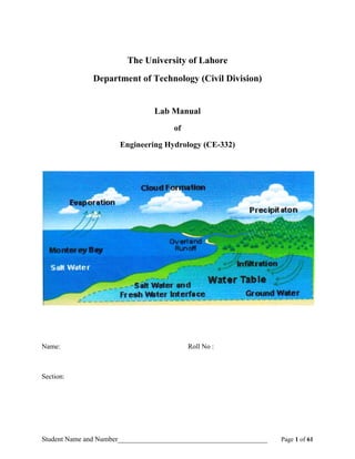
  • 4. Student Name and Number___________________________________________ Page 4 of 61 Design No. 1 To plot a graph for the given data of temperature (T) and saturated vapor pressure (es) of air showing that the saturated vapor pressure is a function of the temperature. Also find the following for the given conditions Saturation Deficit (es – e) Relative Humidity (f) Dew point temperature (Td) Condition No. Air Temperature (T) (°C) Vapor Pressure (e) (mm of Hg) 1 2 3 4 Related Theory Hydrology It is the scientific study of hydrological cycle. Schematic diagram showing the hydrological cycle is presented in Figure 1.1. Figure 1.1: Pictorial view showing the global hydrological cycle.
  • 5. Student Name and Number___________________________________________ Page 5 of 61 Hydrology is the science of waters of the earth, their circulation and distribution over the globe, their physical and chemical properties and their interaction with the physical and biological environment (Aswan N. M. 1981). Hydrology is concerned with the circulation of water and its constituents through the hydrologic cycle. It deals with precipitation, evaporation, infiltration, groundwater flow, runoff, stream flow and the transport of substances dissolved or suspended in flowing water. Hydrology is primarily concerned with water on or near the land surface; ocean waters are the domain of oceanography and the marine sciences (Maidment 1993). Hydrology is an earth science. It encompasses the occurrence, distribution, movement, and properties of the waters of the earth. Knowledge of hydrology is fundamental to decision making process where water is a component of the system of concern. Water and environmental issues are inextricably linked, and it is important to clearly understand how water is affected by and how water affects ecosystem manipulations (Viessman Warren 1996). Engineering Hydrology Engineering hydrology includes those segments of the field pertinent to planning, design and operation of engineering projects for the control and use of water (Linsley 1982). Significance of Hydrology Study of water is extremely necessary as: I. It is the basic need for the sustenance of human life over the planet (drinking, agriculture and industry). II. To cope with the extreme hydrological events (floods and droughts). III. To determine input data for the design of hydraulic structures (Design floods and sediment inflows). Meteorology It is the science of atmosphere which is gaseous envelope surrounding the earth (Awan N. M. 1981).
  • 6. Student Name and Number___________________________________________ Page 6 of 61 Climatic Factors Meteorology of the region is affected by certain climatic factors. I. Amount and distribution of precipitation. II. The occurrence of snow and ice. III. Wind velocity. IV. Temperature. V. Humidity. Importance of Knowledge of Meteorology I. Cloud formation. II. Occurrence of precipitation. III. Thunder storm formation. IV. Movement of rainstorms. V. Weather forecast. VI. As the meteorological phenomena are the forerunners of floods, flood warnings and forecasts may be issued in advance if one can make use of the meteorological conditions that are likely to produce floods. Knowledge of meteorology is also essential prerequisite in the understanding of evaporation phenomenon. Atmosphere Atmosphere is the gaseous envelop around the earth surface. It consists of many gases like N2, O2, CO2 etc and water vapours. The term is derived from the Greek work atoms (vapor of breath) and sphaira (sphere or ball) (Aswan N. M. 1981). Troposphere / Hydrosphere It is the layer of atmosphere adjacent to the surface of the earth, which contains about 99% of total atmospheric water. Its average thickness is about 12 km. For civil engineers this is the most important atmospheric layer. All processes like cloud formation, thunderstorms, and precipitation take place in this layer.
  • 7. Student Name and Number___________________________________________ Page 7 of 61 Figure 1.2: Photograph showing layers of atmosphere and their average thicknesses. Atmospheric Water It is the water available in the atmosphere (troposphere / hydrosphere), in the form of water vapors’, ice crystals, clouds and precipitating particles etc. The quantity of water in atmosphere is approximately 12.900 Km3 , which is about 0.001% of total global water and 0.5% of volume of the atmosphere (Chow 1988). Vaporization It is the process of transformation of water from liquid state to vapor state. The process of vaporization at global scale is shown in Figure 1.3. Figure 1.3: Conceptual diagram showing the phenomenon of evaporation. Vapor Pressure (e) Pressure exerted by the water vapors in air is known as vapors in air is known as paver pressure. Its commonly used units are mm of Hg.
  • 8. Student Name and Number___________________________________________ Page 8 of 61 Graph showing relationship between air temperature and saturation vapor pressure. Saturation Vapor Pressure (es) It is the vapor pressure when air is fully saturated at a given temperature. It is the measure of moisture holding capacity of air, which increases with increase in air temperature as shown in Figure 1.4. Sr. # Air Temperature (°C) Saturated Vapor Pressure (mm of Hg) 1 2 3 4 5 6 7 8 9 10 11 12 13 14 15 16 17 18 19 20
  • 9. Student Name and Number___________________________________________ Page 9 of 61 Saturation Deficit The difference between the saturation vapor pressure and vapor pressure of the air at a given temperature is called saturation deficit. ∆ e = es - e (1.1) Where ∆ e is saturation deficit, es is the saturation vapor pressure and e is the vapor pressure. Humidity It is the presence of moisture in the air. Humidity in the atmosphere can be assessed by vapor pressure of air. Relative Humidity It is the ratio between the vapor pressure and the saturation vapour pressure of air at a given temperature. It is usually expressed in percentage. f = 𝒆 𝒆𝒔 x 100 (1.2) Dew Point Temperature (Td) The dew point temperature can be defined as the temperature at which the air mass just becomes saturated if cooled at constant pressure with moisture neither added nor removed (Awan N. M. 1981). Once air is cooled naturally to this temperature dewdrops are formed. This usually happens at late night when temperature falls significantly.
  • 10. Student Name and Number___________________________________________ Page 10 of 61 Table 1.2: Table of Calculations:- Sr. # Air Temperature (°C) Vapor Pressure (e) (mm O Hg) Saturated Vapor Pressure (es) (mm of Hg) Saturation Deficit (es – e) (mm of Hg) Relative Humidity e f = --------- x 100 es (%) Dew Point Temperature (Td) (°C) 1 2 3 4 Procedure 1. Plot a graph between saturated vapor pressure (es) and air temperature (T) choosing suitable scale. 2. Plot condition 1 for a given e & T on es ~ T graph. 3. For point 1, draw a vertical line passing through the point up to the saturation line, measure distance between saturation line; it is the saturation vapor pressure for point 1. 4. Measure vertical distance between point 1 and saturated line, it is saturation deficit. 5. Compute relative humidity by using equation (1.2). 6. Draw a horizontal line from point 1 to the left, it may intersect with the saturation curve. Note down the temperature for the intersection point, it is the dew point temperature. 7. Repeat steps 2 to 6 for points 2, 3 and 4. Results The results of the design exercise are presented in the last three columns of Table 1.2.
  • 11. Student Name and Number___________________________________________ Page 11 of 61 Comments
  • 12. Student Name and Number___________________________________________ Page 12 of 61 Design No. 2 Annual precipitation at rain gauge ‘X’ and the average annual precipitation at ------- surrounding rain gauges are listed in the following table Examine the consistency of station ‘X’ data. When did the change in the regime occurred? Discuss possible reasons. Adjust the data and determine what difference this makes to the -------- years annual precipitation at station ‘X’. Table 2.1: Observations Year Average Annual PPT. (cm). Station ‘X’ Average of ------- Surrounding Stations
  • 13. Student Name and Number___________________________________________ Page 13 of 61 Related Theory Precipitation All types of moistures reaching to the surface of earth from atmosphere is known as precipitation. The precipitation on land surface is about one 3rd of the total global precipitation. The precipitation on land surface is due to 10% evaporation from land and 90% evaporation from oceans (Chow 1988). Figure 2.1: Climatological station showing various equipment. Forms of Precipitation At a place, precipitation may fall in one or more than one following forms. i. Drizzle or Mist ii. Rain iii. Snow iv. Sleet v. Glaze vi. Hail vii. Fogs viii. Frost ix. Trace
  • 14. Student Name and Number___________________________________________ Page 14 of 61 Drizzle or Mist It is the precipitation in the form of tiny liquid droplets having diameter from 0.1 mm to 0.5 mm. Its intensity rarely increases 1 mm / hr (Linsley 1982). Rain Precipitation in the form of liquid droplets of diameters ranges from 0.5 mm to 6 mm. Its intensity is greater than 1mm /hr. According of U.S.A metrological department rainfall is classified as: a. Light Rain I< 2.5 mm / hr b. Moderate Rain 2.5 mm / hr < I < 7.6 mm / hr c. Heavy Rain I > 7.6 mm / hr Figure 2.2: Standard rain gauge at a Climatological station. Snow It is the precipitation in the form of ice crystals. Specific gravity of fresh fallen snow is approximately 0.1. Sleet It is precipitation in the form of mixture of liquid drops and ice crystals.
  • 15. Student Name and Number___________________________________________ Page 15 of 61 Glaze It is the ice coating generally clear and smooth on exposed surfaces by the freezing of super cooled water deposited by the rain. Hails It is the precipitation in the form of ice balls or lumps. Diameter of hail ranges from 5 mm to 125 mm (Linsley 1982). Figure 2.3: Weather station for the measurement of precipitation, wind speed, wind direction and minimum and maximum temperatures. Fog It is the precipitation in the form of weak cloud clone reaching to the surface of earth. Due to very small size droplets it remains suspended in air for some time. Fog produces a lot a visibility problem. Frost It is the precipitation in the form of frozen dewdrops on the land surface. Trace It is the very small amount precipitation at a remain gauging station, usually less than or equal to 0.125 mm.
  • 16. Student Name and Number___________________________________________ Page 16 of 61 Mechanism To From Precipitation There are four mechanisms necessarily required for the occurrence of precipitation over an area. Lifting Mechanism Water vapor is present in air even in cloudless days. There are three mechanisms available in nature for lifting moisture-laden air to higher levels where condensation is possible due to having very low air temperatures. a. Convective systems b. Orographic barriers c. Cyclones Formation of Cloud Droplets / Ice Crystals Condensation of water vapor into cloud droplets takes place on hygroscopic nuclei or condensation nuclei. These are tiny particles having affinity for water. The sources of these condensation nuclei are the particles of sea salt and products of sulsphurus and nitrous acids (Linsley 1982). Condensation will occur if air in atmosphere is cooled to saturation. Condensation nuclei range in size from 0.1 μ m to 10 μ m. For the formation of ice crystals, freezing nuclei are required which usually consist of clay minerals (Kaolin). Growth of Cloud Droplets / Ice Crystals Cloud elements are generally smaller than 50 μ m in diameter. The droplet size must be large enough for the occurrence of precipitation to overcome the buoyant force and drag force produced due to vertical relative motion between cloud droplet and air. Moreover, cloud elements must also be large enough to penetrate the unsaturated air below the cloud base without evaporating completely. An upward current of less than 0.5 cm / s is sufficient to keep from falling to precipitating droplets have diameters under 10 μ m. Ice crystals of the same weight (larger size) can be
  • 17. Student Name and Number___________________________________________ Page 17 of 61 supported by even lesser velocities. In nature, there are two processes available for the growth of cloud elements. a. Coalescence of Cloud Droplets This is the growth of cloud droplets due to collision of larger drops with smaller one. At an average, 7 collisions take place per km fall of droplet. b. Coexistence of Ice Crystals and Cloud Droplets If in a layer of clouds there is moisture of water droplets and ice crystals, the saturation vapor pressure over ice is lower than over water. As a consequence of this difference there results evaporation of water drops and condensation of much of this water on ice crystals causing their growth and ultimate fall through the clouds. This effect is known as Bergeron’s effect. The ice crystals will further grow as they fall and collide with water droplets. Sufficient Accumulation of Moisture over an Area For the occurrence of heavy precipitation over an area requires heavy water vapor presence in the atmosphere. It needs a large net horizontal inflow of water vapor into the atmosphere above the basin area. This process is called convergence. Rain Gauge It is an instrument used to measure the amount of rainfall or intensity of rainfall at a place. A typical Climatological station is shown in Figure 2.1, a standard rain gauge in Figure 2.2 and a weather station in Figure 2.3 which can measure precipitation, wind speed, wind direction, minimum and maximum temperatures. Amount of Precipitation (mm or inches) It is total depth of rainfall over an area usually in one day.
  • 18. Student Name and Number___________________________________________ Page 18 of 61 Intensity of Precipitation Reference: It is the amount of precipitation at a place per unit time (rain rate). It is usually expressed in mm / hr. Mean / Average Rainfall for N Years It the arithmetic average of annual precipitations for N years over a rain gauging station. Mathematically: (2.1) Where Pavg is the average precipitation, N is the total number of years and Pi is the annual precipitation for ith year. Annual Rainfall Total amount of rainfall accumulated in one year at a place, mathematically it is expressed as: (2.2) Where, Pann is he annual precipitation at a rain gauging station and Pi is the daily precipitation. Average Rainfall over an Area It is amount of precipitation which can be assumed as uniform for the area. It is estimated by using several approaches. One is the arithmetic mean as defined mathematically: (2.3)
  • 19. Student Name and Number___________________________________________ Page 19 of 61 Where, Pavg is the areal average precipitation, N is the total number of stations and Pi is the average annual precipitation for it h station. Reasons of Inconsistency in Precipitation Data Record a. Change in Location of a rain gauge. b. Change of instrument (rain gauge). c. Change in observational procedures. Procedure 1. Calculate cumulative annual precipitation for station ‘X’. 2. Calculate cumulative average annual precipitation of ‘N’ surrounding stations. 3. Plot scatter diagram between cumulative annual precipitation of station ‘X’ and cumulative average annual precipitation of ‘N’ surrounding stations. 4. Joint points carefully with straight lines and note down the intersection point. 5. Determine slopes of the two curves. 6. Compute ratio S1 S2 7. Adjust average annual precipitation of station ‘X’ after the change has occurred. Figure 2.4: Locations of station ‘X’ and surrounding stations in a basin.
  • 20. Student Name and Number___________________________________________ Page 20 of 61 Table 2.1: Computations for Double Mass Analysis Year Annual Precipitation (cm) Cumulative Annual Precipitation (cm) Adjusted Annual PPT at Station ‘X’ (cm) Station ‘X’ Average of 20 Surrounding Stations Station ‘X’ Average of 20 Surrounding Stations Col 1 Col 2 Col 3 Col 4 Col 5
  • 21. Student Name and Number___________________________________________ Page 21 of 61 Results
  • 22. Student Name and Number___________________________________________ Page 22 of 61 Comments
  • 23. Student Name and Number___________________________________________ Page 23 of 61 Design No. 3 The names, locations by latitude and longitude and mean annual precipitations for certain weather stations within and outside the catchment’s area are given below: Name of Stations Latitude (____º____) Longitude ( º____) Mean Annual PPT. (cm) Estimate he average rainfall over the basin area by using following three methods. i. Arithmetic Mean Method ii. Thiessen Polygon Method iii. Isohyetal Method The boundary of the watershed is rectangular and is defined by following four coordinates: A ( ) B ( ) C ( ) D ( )
  • 24. Student Name and Number___________________________________________ Page 24 of 61 Related Theory Average Precipitation over an Area It is the amount of precipitation which can be assumed uniform for the entire area. By simplest method, it can be obtained by adding the precipitations of all stations and dividing by the number of stations in the area or outside the area closer to the boundary. The rain gauges used to measure precipitation are shown in Figure 3.1. Significance of Average Precipitation If average precipitation over an area is known, then it is very easy to compute the total volume of rainfall received by the area for nature. Rainfall volume = Area x Average precipitation.
  • 25. Student Name and Number___________________________________________ Page 25 of 61 Figure 3.1 Showing Rain Guages Figure 3.3 showing Isohyetal Method Figure 3.2 showing Thiessen Polygon Method
  • 26. Student Name and Number___________________________________________ Page 26 of 61 Methods of Finding Average Precipitation over an Area There are three common methods for averaging precipitation over an area. i. Arithmetic Mean Method ii. Thiessen Polygon Method iii. Isohyetal Method Arithmetic Mean Method It is the simplest method of averaging precipitation over an area. This method is applicable where precipitation gauging stations are more or less equally spaced and also precipitation amounts do not vary significantly with each other. The average precipitation over an area by arithmetic mean method is obtained as follows: (3.1) Where N is total number of stations and P1 is mean annual precipitation at ith station. Table 3.1: Average Precipitation by Arithmetic Mean Method:- No. of Stations Name of Stations Mean Annual PPT. (cm)
  • 27. Student Name and Number___________________________________________ Page 27 of 61 Thiessen Polygon Method The fundamental principle followed in this method consists of weighing the value of precipitation at each station by a suitable proportion of basin area. Therefore ppt. data is plotted over a map (graph). The Thiessen polygon map for a typical watershed is shown in Figure 3.2. Procedure 1. Select suitable and same scale for X and Y-axis. 2. Plot catchment’s boundary and station locations. 3. Plot polygons around each strength by connection closest station by straight dashed lines and drawing perpendicular bisectors to make the sides of polygon. 4. Determine area of each polygon by counting the number of squares. 5. Compute product (P1 A1) and sum all products. 6. Compute average precipitation using following equation. (3.2) Where, N is number of polygons within catchments, P1 is the mean annual precipitation for ith polygon and A1 is the area of ith polygon.
  • 28. Student Name and Number___________________________________________ Page 28 of 61 Table 3.2: Table of calculations for Thiessen Polygon Method:- Sr. # Gauging Stations Observed Annual ppt., Pi (cm) Area of Polygon, Ai (min2) Product (Pi Ai) (mm min2) Isohyetal Method Isohyets It is the line representing the same amount of precipitation. In Isohyetal method, area between two consecutive isohyets is determined. Weighted average precipitation for each segment is computed and then average precipitation for the entire basin is determined. The Isohyetal map for a typical watershed is shown in Figure 3.3 and Isohyetal map for annual precipitation over Pakistan is shown in Figure 3.1.
  • 29. Student Name and Number___________________________________________ Page 29 of 61 Procedure i. Select suitable and same scale for X and Y-axis. ii. Plot catchment’s boundary and station locations. iii. Mention precipitation amounts on each station. iv. Select suitable contour interval and number of isohyets. v. Draw isohyets by linear interpolation between stations. vi. Determine area between two consecutive isohyets. vii. Calculate product (Pi Ai). viii. Compute average precipitation by formula. (3.3) Where, N is number of strips / segments, Pi is the mean precipitation for ith strip and Ai is the area of ith strip. Table 3.3: Table of Calculations For Isohyetal Method:- Sr. # Isohyetal Precipitation (mm) Mean ppt. (mm) Area of Strip (min2) (mm. min2)
  • 30. Student Name and Number___________________________________________ Page 30 of 61 Result The average annual precipitation for the watershed is: Pavg = mm by using mean arithmetic method. Pavg = mm by using Thiessen polygon method. Pavg = mm by using Isohyetal method.
  • 31. Student Name and Number___________________________________________ Page 31 of 61 Comments
  • 32. Student Name and Number___________________________________________ Page 32 of 61 Design No. 4 Given below are data for a station rating curve. Extend the relation and estimate the flow at a stage of (------m) by logarithmic and Chezy’s methods: Sr. # Stage, H (m) Mean Depth, D (m) X-Sec Area A (m2) Discharge, Q (m3/sec).
  • 33. Student Name and Number___________________________________________ Page 33 of 61 Related Theory Stage Stage is the height of the water surface above an arbitrary datum. In Figure 4.1 stage (H) and depth (d) are shown on a stream section. Stage Gauge The instrument used for measuring stage at a gauging station is called stage gauge. The staff stage gauges at a stream gauging station are shown in Figure 4.2. Types of Gauges There are two main types of stage gauges, i.e. Non-recording stage gauges and recording gauges. Non-recording stage gauges are those, which do not record the stage values automatically. The examples are staff stage gauge, wire weigh gauge etc. Figure 4.1: Conceptual diagram showing the measurement of stage in a stream. Recording stage gauges keep the record of stages automatically for a particular duration of time say one day. The example is the float type stage gauge.
  • 34. Student Name and Number___________________________________________ Page 34 of 61 Figure 4.2: Staff stage gauges at a stream gauging station. Rating Curve It is a graphical relationship between stage and discharge at a stream gauging station as shown in Figure 4.3. Flow (cumics) Figure 4.3: A typical rating curve for a stream gauging station. Significance of Rating Curve
  • 35. Student Name and Number___________________________________________ Page 35 of 61 i. To get discharge value corresponding to any stage value. ii. To determine stage values corresponding to various flows for the construction of hydraulics structures. Figure 4.4: Graphical procedure for the extension of rating curve using Logarithmic Method. How a Rating Curve is established at a Site It is plotted by taking simultaneous measurements of stage and discharge at different water levels (stages) in the steam at a particular section. The cross sectional area of flow is divided in a number of segments assigning that in a particular segment the velocity remains uniform in width. Velocity of flow is measured in each segment with the help of current meter. Then discharge is computed in each segment and total discharge is determined by integrating it for the entire cross section. Figure 4.5: Graphical procedure for the extension of rating curve using Chezy’s Method.
  • 36. Student Name and Number___________________________________________ Page 36 of 61 Extension of Rating Curve Rating curves are established by collecting and plotting past data of stages and discharges for a particular section of the stream. A flood magnitude (for higher returned periods) is expected at any time in future greater than the highest observed in the past and the available rating curve becomes useless for this value of flood stage. Then extension of rating curve becomes essential to determine the flood magnitude on a value of the stage higher than the observed. Methods of Extension of Rating Curve Usually, there are two approaches for the extension of rating curve. a. The logarithmic method. b. Chezy’s method. The Logarithmic Method This method is used if the cross section of the steam at the gauging station is of regular shape. Log Q = Log K + n log (H – a) Chezy’s Method This method is based on Chezy’s equation. Q = AC √ RS If the friction is uniform and bed slope S is constant Q = AC √ S √ R R= A P = bD b + 2D ≈D Q = A (C√ S) √ D Q = (C√ S) A √ D Q oc A √ D Where b is the bed width, D is the mean depth of the stream, R is the hydraulic radius, S is the slope of the energy line and Q is the flow rate in the channel. As flow is proportional to the A
  • 37. Student Name and Number___________________________________________ Page 37 of 61 √ D , hence the graphical relationship between them should definitely be an straight line, which can be easily extended up to required stage value. The graphical procedure required for the extension of rating curve by Chezy’s method is shown in Figure 4.5. Table 4.1: Table of Calculations For The Extension of Rating Curve. Sr.# Stage H (m) Depth D (m) Area A (m3 ) Discharge Q (cumics) A√ D (m2.5 ) LogQ Log (H-a) a= a= a=
  • 38. Student Name and Number___________________________________________ Page 38 of 61 Results i. Flood magnitude, Q at ------m stage by logarithmic method is --------- m3/ S. ii. Flood magnitude, Q at ------m stage by Chezy’s method is -------------- m3/ S. Comments
  • 39. Student Name and Number___________________________________________ Page 39 of 61 Design No. 5 Following are the ordinates of a storm hydrograph for a river draining catchments area of ----------- km2 due to a ---------- hours isolated storm. Drive the ordinates of --------- hour’s unit hydrograph for the catchment. Time From Start (Hours) Discharge (m3 / sec)
  • 40. Student Name and Number___________________________________________ Page 40 of 61 Related Theory Hydrograph It is the graphical representation of flow against time for a particular section of the stream / river.. Variable kept on y-axis is flow or discharge while on x-axis it is time. Parts of Hydrograph Hydrograph comprises of the following four parts. i. Ground water recession curve. ii. Rising limb. iii. Peak iv. Recession curve or falling limb. Components of a Hydrograph i. Direct runoff (DRO) ii. Base flow Factors Affecting the Shape of Hydrograph The main factors affecting the shape of hydrograph are basically two, the climatic factors and second are the physiographical factors. Climatic factors include the amount of rainfall, intensity and duration of rainfall, while physical characteristics of the watershed include the shape of the basin, slope of the watershed, surface conditions of the catchment and soil types in the watershed. Hydrograph Separation The hydrograph separation means splitting the hydrograph ordinates in two parts i.e. the base flow and direct runoff (DRO) ordinates. Methods of Separation of Hydrograph Following are the methods used for the separation of hydrographs.
  • 41. Student Name and Number___________________________________________ Page 41 of 61 1. Straight line method. a. Horizontal straight line method b. Inclined line method 2. Fixed base length method 3. Variable slope method In horizontal straight line method a horizontal line is drawn from the point of rise. The area below the line is base flow. This line is based on the assumption that a constant amount of base flow is maintained during the storm runoff. It produces an extremely long time base for the DRO. In inclined line method, inclined line is obtained by joining two points, i.e. Where DRO enters and where DRO ceases. DRO ceases after N days from the pack discharge and is obtained by the following relationship. N = K (A) 0.2 Where N is the time in days after which DRO ceases from the peak and depends on the basin characteristics, A is the area of the watershed and K is the coefficient, its value is 1 for area A in Ml2 and 0.8 for A in km2, respectively. In fixed base length method, a line AB is drawn in the extension of groundwater recession curve ending at peak of the hydrograph (B). Another line BC is drawn from point B to C where DRO ceases at a distance of N days from the peak of hydrograph. The area of hydrograph above curve ABC is DRO and below is base flow (Linsley 1982). Unit Hydrograph It is the direct runoff hydrograph with unit effective precipitation over the entire watershed. Applications of Unit Hydrograph A unit hydrograph is used for the prediction of flood peak and time to peak in the stream at a particular section due to any amount of effective precipitation over the watershed. Assumptions For the UGH i Precipitation amount and intensity is uniform over the entire watershed. ii. Precipitation intensity remains uniform though out the storm.
  • 42. Student Name and Number___________________________________________ Page 42 of 61 iii. Base length of hydrograph DRO for a particular catchments resulting from a storm of a given duration is approximately constant. iv. Entire watershed is treated as a single unit. Procedure i. Plot hydrograph of given data. ii. Separate base flow and DRO. iii. Determine volume of DRO in km3 or cft. iv. Determine volume of DRO in cm or inches (x) by dividing the volume with watershed area. v. Compute ordinates of UHG ordinates = ordinates of DRO / X. vi. Plot unit hydrograph. vii. Check area under the curve of UHG, it should be 1 cm or 1 inch depending on the system of units used. Equation?
  • 43. Student Name and Number___________________________________________ Page 43 of 61 Table 5.1: Derivation of the ordinates of unit hydrograph:- Time For Start (Hours) Discharge (m3 / sec) Base Flow (m3 / sec) DRO (m3 / sec) Ordinates of Unit Hydrograph (DRO / x) Check for area under UHG =? The area under UHG in cm is = ?
  • 44. Student Name and Number___________________________________________ Page 44 of 61 Results Comments
  • 45. Student Name and Number___________________________________________ Page 45 of 61 Design No. 6 The ordinates of a ------- hrs unit hydrograph are given below. Derive the ordinates of: S-curve hydrograph -------- hrs unit hydrograph -------- hrs unit hydrograph Time (hrs) Ordinates of ------ hrs Unit Hydrograph (m3 /s) Time (hrs) Ordinates of ------ hrs Unit Hydrograph (m3 /s)
  • 46. Student Name and Number___________________________________________ Page 46 of 61 Related Theory General Any unit hydrograph for a catchment is associated with definite duration of rainfall and hence cannot be used for all durations. It is therefore necessary to derive unit hydrograph of various durations. For this purpose it is not essential to use the actual rainfall data and the flood hydrograph because a short duration unit hydrograph can be converted into a long or vice versa by S-curve method provided other durations are integral multiple of given duration. Thus for example S- curve method can be used to develop 12 hours unit hydrograph from a 4 hr unit hydrograph. It is also called as conversation of UGH duration. S-Curve The S-curve is a hydrograph of surface runoff, which result from an addition of an infinite series of T hr unit hydrograph each lagged by T hours (i.e. equal to the duration of the stream) with respect to the preceding one. The S-curve becomes consultant after a period equal to the base length of the unit hydrograph used to derive it. Methods For S-Curve Generation Following methods can be used for the derivation of S-curve ordinates. 1. Offset method. 2. S-curve addition method.
  • 47. Student Name and Number___________________________________________ Page 47 of 61 Table 6.1: Derivation of S-Curve Ordinates by Offset Method Time (hrs) Ordinates of ----- hrs UHG (m3 /s) Off Set Ordinates of S-Curve (m3 /s) 1 2 3 4 5 Table 6.2: Derivation of S-Curve, --------- hrs UHG and ---------- hrs UHG Ordinates
  • 48. Student Name and Number___________________________________________ Page 48 of 61 Time (hrs) Ordinate s of ----- hrs UHG (m3 /s) S-Curve Addition al (m3 /s) Ordinate s of S- Curve (m3 /s) S- Curve Lagge d by -- - hrs (m3 /s) Diff. of col. (4) & col. (5) (m3 /s) Ordinates of ----- hrs UHG (m3 /s) S- Curve Lagged by --- hrs (m3 /s) Diff. of col. (4) & col. (8) (m3 /s) Ordin ates of ---- - hrs UHG (m3 /s) Col.(1) Col.(2) Col.(3) Col.(4) Col.(5) Col.(6) Col.(7) Col.(8) Col.(9) Col.(1 0)
  • 49. Student Name and Number___________________________________________ Page 49 of 61 Procedure
  • 50. Student Name and Number___________________________________________ Page 50 of 61 Results Comments
  • 51. Student Name and Number___________________________________________ Page 51 of 61 Design No. 7 The thickness of a horizontal, confined, homogeneous isotropic aquifer of infinite areal extent is ------ m. A well fully penetrating the aquifer was continuously pumped at a constant rate of ------ m3/sec for a period of 1 day. The drawdown given in the table were observed in a fully penetrating well ------ m from the pumping well. Compute the transmissivity (T) and storativity (S) by using Thiess method. Time (min) Drawdown (m) Time (min) Drawdown (m)
  • 52. Student Name and Number___________________________________________ Page 52 of 61 Related Theory Aquifer An aquifer is a water-bearing stratum or formation capable of transmitting water in quantities sufficient to permit development. Aquifers may be considered as falling into two categories, confined and unconfined, depending on whether a water table or free surface exists under atmospheric pressure. Storage volume within an aquifer is changed whenever water is recharged to, or discharged from, an aquifer (Viessman 1996). Unconfined Aquifer The top most water bearing strata having no confining impermeable overburden is known as unconfined aquifer. This aquifer is also known as non-artesian aquifer or water table aquifer. A special case of unconfined aquifer involves perched water bodies. This occurs whereas a ground water body is separated from main water table by relatively impermeable stratum as shown in Figure 7.1. Figure 7.1: Schematic diagram showing the perched water table.
  • 53. Student Name and Number___________________________________________ Page 53 of 61 Confined Aquifer It is such an aquifer which remains over laden by an impermeable strata or aquiclude. The water is under reassure in this aquifer, confined aquifers are also known as artesian aquifers. Figure 7.2 shows the confined and unconfined aquifers. Figure 7.2: A typical diagram showing confined and unconfined aquifers. Hydraulic Conductivity It is the discharge through a porous medium for unit cross sectional area under unit hydraulic gradient. It is also called coefficient of permeability. According to Darcy’s equation. K = 𝑄 i A Where, Q is the flow rate, I is the hydraulic gradient, A is the cross sectional area and K is the hydraulic conductivity. Transmissivity A storage coefficient (or storativity) is defined as the volume of water that an aquifer releases from or takes into storage per unit surface area of aquifer per unit change in head normal to that surface. It is product of specific storage Ss and thickness of aquifer b.S = Ss
  • 54. Student Name and Number___________________________________________ Page 54 of 61 Hydraulic of Well When a well is pumped, water is removed from the aquifer surrounding the well and the water table is lowered. This lowering takes place in a well as well as surrounding the well. This depression is called drawdown curve. A drawdown curve shows the variation of drawdown with distance from the well. In 3 D, the drawdown curve has a conic shape known as cone of depression. Also the outer limit of cone of depression defines the area of influence of the well (Linsley 1982). In unsteady state condition, drawdown changes significantly with time, whereas in steady state condition it changes negligibly with time. When a well penetrating an extensive confined aquifer is pumped at a constant rate, the influence of the discharge extends outward with time. The rate of decline of head time the storage coefficient summed over the area of influence equals the discharge. Because the water must come from the reduction of storage within the aquifer, the head will continue to decline as long as the aquifer is effectively infinite, therefore, unsteady, or transient, flow exists. The rate of decline, however, decreases continuously as the area of influence expands. Figure 7.3: Schematic diagram showing the field arrangement for pumping well and observation well used in Thiess method. There are two major formulae are available for the solution of the well problem i.e. Thiem formula and Thiess formula. Thiem / equilibrium well formula is used for the steady state flow condition and requires two observation wells. Thiess formula / non-equilibrium well formula is used for unsteady flow condition.
  • 55. Student Name and Number___________________________________________ Page 55 of 61 Thiess Formula Thiess formula in simplified form for the solution of confined aquifer with unsteady flow condition based on graphical method of superposition is given below: Where, S is the storativity, Q is the flow rate, T is the transmissivity, r is the radius or distance between observation well and pumping well, t is the time and W (u) is the well function of u and its numerical values are given in Table 7.1. Assumptions of Thiess Method 1. Aquifer is homogenous, isotropic, of uniform thickness and infinite areal extent. 2. Before pumping, piezometric surface is horizontal. 3. Well is pumped at a constant discharge rate. 4. Flow everywhere is horizontal within the aquifer to the well. 5. Storage within well can be neglected (small well diameter). Merits of Thiess Method 1. A value of S can be determined. 2. Only one observation well is required. 3. A shorter period of pumping is required. 4. No assumption of steady state flow condition is required.
  • 56. Student Name and Number___________________________________________ Page 56 of 61 Table 7.1: Values of W (u) for various values of u (Viessman 1996):- u 1.0 2.0 3.0 4.0 5.0 6.0 7.0 8.0 9.0
  • 57. Student Name and Number___________________________________________ Page 57 of 61 Procedure
  • 58. Student Name and Number___________________________________________ Page 58 of 61 Table 7.2: Table of Calculations Sr. # Drawdown, s (m) r2 (m2 / min) t Sr. # Drawdown, s (m) r2 (m2 / min) t
  • 59. Student Name and Number___________________________________________ Page 59 of 61
  • 60. Student Name and Number___________________________________________ Page 60 of 61
  • 61. Student Name and Number___________________________________________ Page 61 of 61 Results Comments