Downloaded 754 times
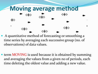

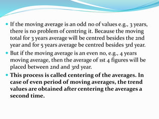
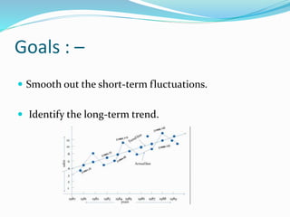
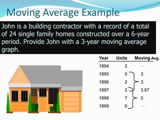
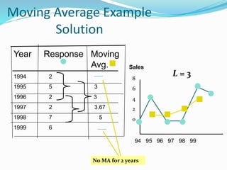
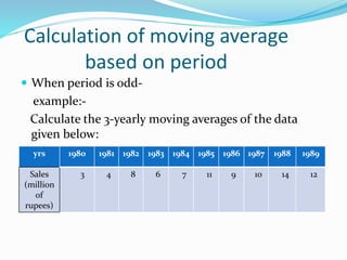
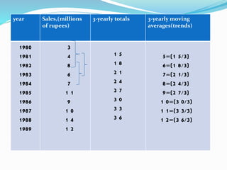
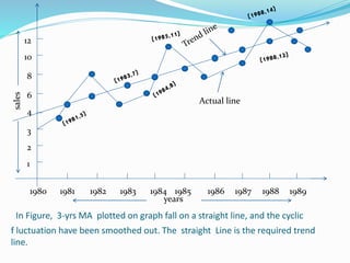
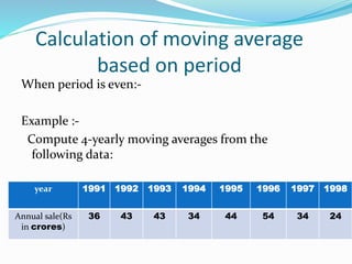
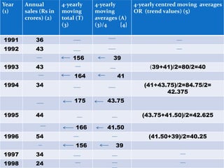

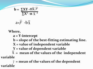
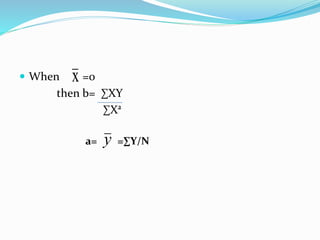
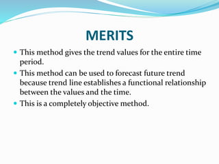
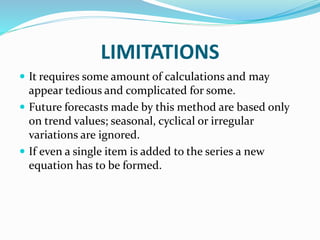
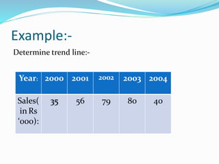
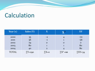
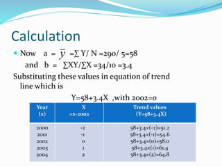
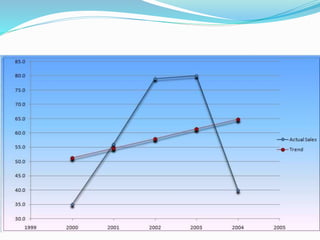
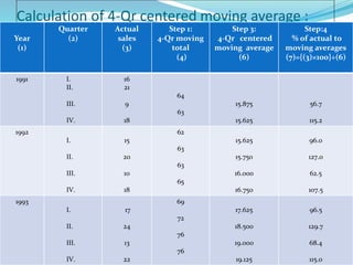
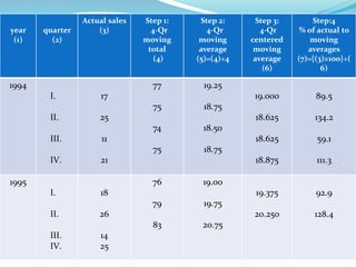
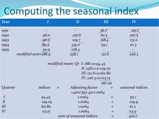
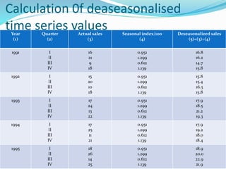
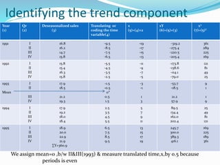
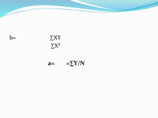
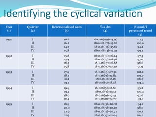
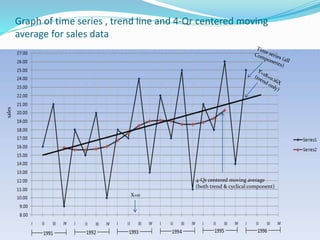


The document discusses the moving average method for forecasting or smoothing time series data. It explains that a moving average is calculated by averaging successive data points over a set time period, with old data dropped as new data is added. The document outlines how to calculate moving averages for both odd and even time periods. It also discusses the merits and limitations of the moving average method, and provides an example calculation.


