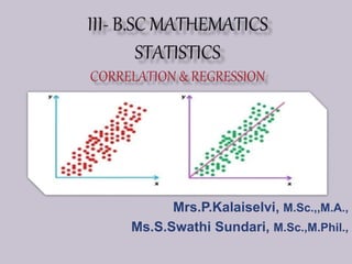
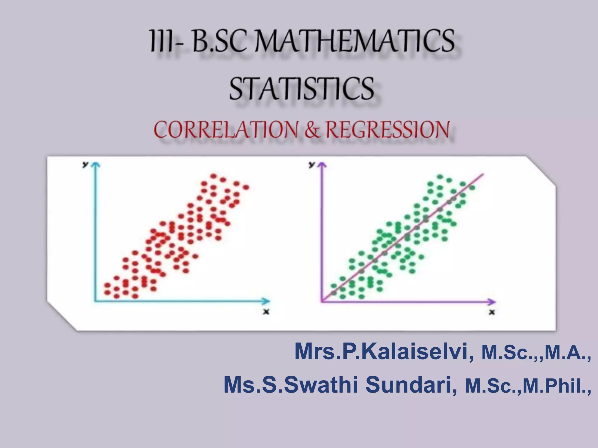
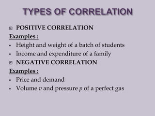
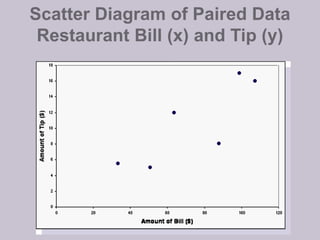
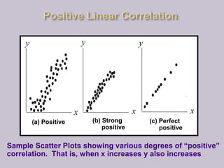
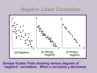
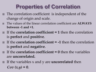
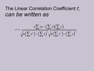
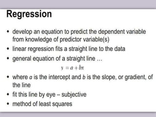
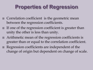
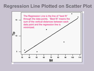
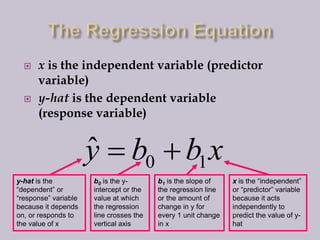
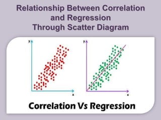
This document discusses linear correlation and regression analysis. It defines correlation as the degree of linear association between two quantitative variables. Positive correlation means both variables increase together, while negative correlation means one variable increases as the other decreases. The correlation coefficient r quantifies the strength of linear correlation between -1 and 1, where -1 is perfect negative correlation, 1 is perfect positive correlation, and 0 is no correlation. The regression line represents the linear relationship that best predicts the response variable y from the predictor variable x.

1. Mrs.P.Kalaiselvi, M.Sc.,,M.A.,
Ms.S.Swathi Sundari, M.Sc.,M.Phil.,

2. Assumptions :
1. The sample of paired data (x,y) is a
random sample.
2. The pairs of (x,y) data are normally
distributed.

3.  Measures the degree of linear association
between two scaled variables analysis of the
relationship between two quantitative outcomes,.

4.  Scatterplot (or scatter diagram)
is a graph in which the paired
(x,y) sample data are plotted with
a horizontal x axis and a vertical
y axis. Each individual (x,y) pair
is plotted as a single point.

5.  POSITIVE CORRELATION
Examples :
 Height and weight of a batch of students
 Income and expenditure of a family
 NEGATIVE CORRELATION
Examples :
 Price and demand
 Volume v and pressure p of a perfect gas

7. Scatter Diagram of Paired Data
Restaurant Bill (x) and Tip (y)

8. x x
yy y
x
Sample Scatter Plots showing various degrees of “positive”
correlation. That is, when x increases y also increases
(a) Positive (b) Strong
positive
(c) Perfect
positive

9. x x
yy y
x
(d) Negative (e) Strong
negative
(f) Perfect
negative
Sample Scatter Plots showing various degrees of
“negative” correlation. When x increases y decreases

10. x x
yy
(g) No Correlation (h) Nonlinear Correlation
Sample Scatter Plots showing NO linear correlation. The first plot (g)
has no correlation of any kind. The other plot (h) shows a clear
correlation between x and y, but the correlation is NOT LINEAR.
Nonlinear correlation can be studied, but it is beyond this class. We
will only study LINEAR CORRELATION.

11.  The correlation coefficient is independent of the
change of origin and scale.
 The values of the linear correlation coefficient are ALWAYS
between -1 and +1.
 If the correlation coefficient = 1 then the correlation
is perfect and positive.
 If the correlation coefficient = -1 then the correlation
is perfect and negative.
 If the correlation coefficient = 0 then the variables
are uncorrelated.
 If the variables x and y are uncorrelated then
Cov (x,y) = 0.

12. The Linear Correlation Coefficient r,
can be written as
  
       
2 22 2
n xy x y
r
n x x n y y


 
  
   

14.  Correlation coefficient is the geometric mean
between the regression coefficients.
 If one of the regression coefficient is greater than
unity the other is less than unity.
 Arithmetic mean of the regression coefficients is
greater than or equal to the correlation coefficient.
 Regression coefficients are independent of the
change of origin but dependent on change of scale.

15. Regression Line Plotted on Scatter Plot
The Regression Line is the line of “best fit”
through the data points. “Best fit” means the
sum of the vertical distances between each
data point and the regression line is
minimized.

16.  x is the independent variable (predictor
variable)
 y-hat is the dependent variable
(response variable)
0 1
ˆy b b x 
b0 is the y-
intercept or the
value at which
the regression
line crosses the
vertical axis
b1 is the slope of
the regression line
or the amount of
change in y for
every 1 unit change
in x
y-hat is the
“dependent” or
“response” variable
because it depends
on, or responds to
the value of x
x is the “independent”
or “predictor” variable
because it acts
independently to
predict the value of y-
hat