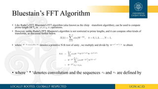
FAST FOURIER TRANSFORM
ANALYSIS
SUB-JUDUL PRESENTASI (SEGOE UI LIGHT)
Thevin Yoga Raditya 15/379077/TK/43019
Satrio Eko W 15/379073/TK/43015
Nico pradipta gunawan 15/379066/TK/43008
Suryanto 15/379074/TK/43016
What is FFT Analysis?
Before we get into FFT Analysis, we should know first: what is Fourier Transform?
Fourier Transform is a tool to transforming a wave function or signal from a time
domain(how a signal changes over time) into frequency domain (how much of the
signal lies within each given frequency band over a range of frequencies)
What is.. continued
To really able to convert the discrete time domain signal to frequency
domain signal, we need Discrete Fourier Transform or DFT. Because the
signal produced by many phenomena is needed to be converted into
frequency domain for easier analysis, but from the measurement we got
the time domain data.
Without DFT we couldn’t separated a compound signal or wave function
of vibration found in a complex mechanism in a system. But DFT is such
a manual way of converting signal from time domain to frequency
domain.
What is.. continued
If the system is so complex, that each part has it’s own natural
frequency, we need and algorithm of DFT to make vibration analysis
much simpler and understandable.
For fulfilling that purpose, the FFT is discovered. Fast Fourier Transform
(FFT) isn’t a new or different way of DFT but it’s an very efficient
algorithm to make computer doing the DFT in a much shorter time. FFT
is able to divide a compound complex signal to a simpler frequency
domain signal, as shows below
What is.. continued
With the FFT, the original complex signal time
domain obtained from measurement (red) could be
simplified by converting it into frequency domain
(blue). Each frequency will contain the number of
signal lies within its frequency band.
With this frequency domain we could see the
amplitudes of each frequencies existed.
In vibration engineering, each part of a system
have is own frequency, and the amplitude of each part
can be monitored by the graphic, if some part goes
wrong, the could analize it from the deviation from
normal amplitude of its frequency.
Type of Fast Fourier
Transform
Cooley–Tukey Fast Fourier Transform
• Simple Cooley-Tukey algorithm is a variant of Fast Fourier
Transform intended for complex vectors of power-of-two size and
avoiding special techniques used for sizes equal to power of 4, power
of 8, etc. The algorithm repeatedly applies the Fast Fourier Transform
and reduces the entire process to a sequence of Fourier transforms of
size 2 and multiplications by the so-called twiddle factors. It is slower
than Cooley-Tukey algorithms that express a power-of-two size as a
power of 4, power of 8, etc. and then use special features of these
cases. Nevertheless, this algorithm is widespread for the reason that
its program implementation is the simplest of all FFT
implementations.
Prime Factor Algorithm
• By the prime factorization theorem, every integer can be uniquely factored
into a product of prime number raised to an integer power :
• As discussed above, a mixed-radix Cooley Tukey FFT can be used to
implement a length N DFTusing DFTs of length . However, for factors
of N that are mutually prime (such as and for ), a more
efficient prime factor algorithm (PFA), also called the Good-
Thomas FFT algorithm,
Bruun’s FFT Algorithm
• Bruun's algorithm is a Fast Fourier Transform (FFT) algorithm based on an
unusual recursive polynomial-factorization approach, proposed for powers of two
by G. Bruun in 1978 and generalized to arbitrary even composite sizes by H.
Murakami in 1996. Because its operations involve only real coefficients until the
last computation stage, it was initially proposed as a way to efficiently compute
the discrete Fourier transform (DFT) of real data. Nevertheless, Bruun's algorithm
illustrates an alternative algorithmic framework that can express both itself and the
Cooley–Tukey algorithm, and thus provides an interesting perspective on FFTs that
permits mixtures of the two algorithms and other generalizations.
• where mod denotes the polynomial remainder operation. The key to fast algorithms like
Bruun's or Cooley–Tukey comes from the fact that one can perform this set
of N remainder operations in recursive stages.
Rader’s Algorithm
The basic idea of Rader’s algorithm is to make use of the special
permutation structure of the powers of ωp in Fp to write the DFT
summation
The first thing we do is to split out the special zero-index parts of the
Fourier matrix calculation, becomes
Bluestain’s FFT Algorithm
• Like Rader’s FFT, Bluestain’s FFT algorithm (also known as the chirp -transform algorithm), can be used to compute
prime-length DFTS in operations.
• However, unlike Rader's FFT, Bluestein's algorithm is not restricted to prime lengths, and it can compute other kinds of
transforms, as discussed further below.
• where denotes a primitive N th root of unity , we multiply and divide by to obtain
• where ‘ * ‘denotes convolution and the sequences and are defined by
Characteristic
FFT computes the DFT and produces exactly the same result as evaluating the DFT definition directly;
the most important difference is that an FFT is much faster.
With the function of : Xc = 𝑛=0
𝑁−1
(𝑥 𝑛 𝑒−
𝑖2𝜋𝑘𝑛
𝑁 ) k=0,.....,N-1
Evaluating this definition directly requires O(N2) operations: there are N outputs Xk, and each output
requires a sum of N terms. An FFT is any method to compute the same results in O(N log N) operations.
All known FFT algorithms require Θ(N log N) operations, although there is no known proof that a lower
complexity score is impossible.
There are several characteristic of FFT regarding :
• Approximation
• Accuracy
• Bounds on complexity and operation counts
Characteristic
Approximation of FFT is exactly as the DFT, such as neglecting the floating
point error. But the error can be made small with increase computation.
Accuracy even the "exact" FFT algorithms have errors when finite-precision
floating-point arithmetic is used, but these errors are typically quite small; most
FFT algorithms, e.g. Cooley–Tukey, have excellent numerical properties as a
consequence of the pairwise summation structure of the algorithms. The upper
bound on the relative error for the Cooley–Tukey algorithm is O(ε log N),
compared to O(εN3/2) for the naïve DFT formula. (Gentleman Dande 1966)
Characteristic
Bounds on complexity and operation counts: A fundamental
question of longstanding theoretical interest is to prove lower
bounds on the complexity and exact operation counts of fast
Fourier transforms, and many open problems remain. It is not even
rigorously proved whether DFTs truly require Ω(N log N) (i.e., order
N log N or greater) operations, even for the simple case of power of
two sizes, although no algorithms with lower complexity are known.
Characteristic of application
• Fast large integer and polynomial multiplication.
• Efficient matrix-vector multiplication for Toeplitz, circulant and other structured
matrices.
• Filtering algorithms.
• Fast algorithms for discrete cosine or sine transforms (example, Fast DCT used for
JPEG, MP3/MPEG encoding)
• Fast Chebyshev approximation.
Spectrum
The FFT spectrum analyzer samples the input signal, computes the magnitude
of its sine and cosine components, and displays the spectrum of these measured
frequency components.
The spectrum is the basic measurement of an FFT analyzer. It is simply the
complex FFT. Normally, the magnitude of the spectrum is displayed. The magnitude is
the square root of the FFT times its complex conjugate. (Square root of the sum of the
real (sine) part squared and the imaginary (cosine) part squared.) The magnitude is a
real quantity and represents the total signal amplitude in each frequency bin,
independent of phase.
Spectrum
If there is phase information in the spectrum, i.e. the time record is triggered in
phase with some component of the signal, then the real (cosine) or imaginary (sine)
part or the phase may be displayed. The phase is simply the arctangent of the ratio of
the imaginary and real parts of each frequency component. The phase is always
relative to the start of the triggered time record.
To illustrate how an FFT can be used, let’s build a simple waveform with and
use an FFT for vibration analysis. This constructed waveform will consist of three
different frequency components: 22 Hz, 60 Hz, and 100 Hz. These frequencies will
have an amplitude of 1g, 2g, and 1.5g respectively. The following figure shows how
this waveform looks a little confusing in the time domain and also illustrates how the
signal length affects the frequency resolution of the FFT.
Spectrum

Fft analysis

  • 1.
    FAST FOURIER TRANSFORM ANALYSIS SUB-JUDULPRESENTASI (SEGOE UI LIGHT)
  • 2.
    Thevin Yoga Raditya15/379077/TK/43019 Satrio Eko W 15/379073/TK/43015 Nico pradipta gunawan 15/379066/TK/43008 Suryanto 15/379074/TK/43016
  • 3.
    What is FFTAnalysis? Before we get into FFT Analysis, we should know first: what is Fourier Transform? Fourier Transform is a tool to transforming a wave function or signal from a time domain(how a signal changes over time) into frequency domain (how much of the signal lies within each given frequency band over a range of frequencies)
  • 4.
    What is.. continued Toreally able to convert the discrete time domain signal to frequency domain signal, we need Discrete Fourier Transform or DFT. Because the signal produced by many phenomena is needed to be converted into frequency domain for easier analysis, but from the measurement we got the time domain data. Without DFT we couldn’t separated a compound signal or wave function of vibration found in a complex mechanism in a system. But DFT is such a manual way of converting signal from time domain to frequency domain.
  • 5.
    What is.. continued Ifthe system is so complex, that each part has it’s own natural frequency, we need and algorithm of DFT to make vibration analysis much simpler and understandable. For fulfilling that purpose, the FFT is discovered. Fast Fourier Transform (FFT) isn’t a new or different way of DFT but it’s an very efficient algorithm to make computer doing the DFT in a much shorter time. FFT is able to divide a compound complex signal to a simpler frequency domain signal, as shows below
  • 6.
    What is.. continued Withthe FFT, the original complex signal time domain obtained from measurement (red) could be simplified by converting it into frequency domain (blue). Each frequency will contain the number of signal lies within its frequency band. With this frequency domain we could see the amplitudes of each frequencies existed. In vibration engineering, each part of a system have is own frequency, and the amplitude of each part can be monitored by the graphic, if some part goes wrong, the could analize it from the deviation from normal amplitude of its frequency.
  • 7.
    What is.. continued Withthe FFT, the original complex signal time domain obtained from measurement (red) could be simplified by converting it into frequency domain (blue). Each frequency will contain the number of signal lies within its frequency band. With this frequency domain we could see the amplitudes of each frequencies existed. In vibration engineering, each part of a system have is own frequency, and the amplitude of each part can be monitored by the graphic, if some part goes wrong, the could analize it from the deviation from normal amplitude of its frequency.
  • 8.
    Type of FastFourier Transform
  • 9.
    Cooley–Tukey Fast FourierTransform • Simple Cooley-Tukey algorithm is a variant of Fast Fourier Transform intended for complex vectors of power-of-two size and avoiding special techniques used for sizes equal to power of 4, power of 8, etc. The algorithm repeatedly applies the Fast Fourier Transform and reduces the entire process to a sequence of Fourier transforms of size 2 and multiplications by the so-called twiddle factors. It is slower than Cooley-Tukey algorithms that express a power-of-two size as a power of 4, power of 8, etc. and then use special features of these cases. Nevertheless, this algorithm is widespread for the reason that its program implementation is the simplest of all FFT implementations.
  • 10.
    Prime Factor Algorithm •By the prime factorization theorem, every integer can be uniquely factored into a product of prime number raised to an integer power : • As discussed above, a mixed-radix Cooley Tukey FFT can be used to implement a length N DFTusing DFTs of length . However, for factors of N that are mutually prime (such as and for ), a more efficient prime factor algorithm (PFA), also called the Good- Thomas FFT algorithm,
  • 11.
    Bruun’s FFT Algorithm •Bruun's algorithm is a Fast Fourier Transform (FFT) algorithm based on an unusual recursive polynomial-factorization approach, proposed for powers of two by G. Bruun in 1978 and generalized to arbitrary even composite sizes by H. Murakami in 1996. Because its operations involve only real coefficients until the last computation stage, it was initially proposed as a way to efficiently compute the discrete Fourier transform (DFT) of real data. Nevertheless, Bruun's algorithm illustrates an alternative algorithmic framework that can express both itself and the Cooley–Tukey algorithm, and thus provides an interesting perspective on FFTs that permits mixtures of the two algorithms and other generalizations. • where mod denotes the polynomial remainder operation. The key to fast algorithms like Bruun's or Cooley–Tukey comes from the fact that one can perform this set of N remainder operations in recursive stages.
  • 12.
    Rader’s Algorithm The basicidea of Rader’s algorithm is to make use of the special permutation structure of the powers of ωp in Fp to write the DFT summation The first thing we do is to split out the special zero-index parts of the Fourier matrix calculation, becomes
  • 13.
    Bluestain’s FFT Algorithm •Like Rader’s FFT, Bluestain’s FFT algorithm (also known as the chirp -transform algorithm), can be used to compute prime-length DFTS in operations. • However, unlike Rader's FFT, Bluestein's algorithm is not restricted to prime lengths, and it can compute other kinds of transforms, as discussed further below. • where denotes a primitive N th root of unity , we multiply and divide by to obtain • where ‘ * ‘denotes convolution and the sequences and are defined by
  • 15.
    Characteristic FFT computes theDFT and produces exactly the same result as evaluating the DFT definition directly; the most important difference is that an FFT is much faster. With the function of : Xc = 𝑛=0 𝑁−1 (𝑥 𝑛 𝑒− 𝑖2𝜋𝑘𝑛 𝑁 ) k=0,.....,N-1 Evaluating this definition directly requires O(N2) operations: there are N outputs Xk, and each output requires a sum of N terms. An FFT is any method to compute the same results in O(N log N) operations. All known FFT algorithms require Θ(N log N) operations, although there is no known proof that a lower complexity score is impossible. There are several characteristic of FFT regarding : • Approximation • Accuracy • Bounds on complexity and operation counts
  • 16.
    Characteristic Approximation of FFTis exactly as the DFT, such as neglecting the floating point error. But the error can be made small with increase computation. Accuracy even the "exact" FFT algorithms have errors when finite-precision floating-point arithmetic is used, but these errors are typically quite small; most FFT algorithms, e.g. Cooley–Tukey, have excellent numerical properties as a consequence of the pairwise summation structure of the algorithms. The upper bound on the relative error for the Cooley–Tukey algorithm is O(ε log N), compared to O(εN3/2) for the naïve DFT formula. (Gentleman Dande 1966)
  • 17.
    Characteristic Bounds on complexityand operation counts: A fundamental question of longstanding theoretical interest is to prove lower bounds on the complexity and exact operation counts of fast Fourier transforms, and many open problems remain. It is not even rigorously proved whether DFTs truly require Ω(N log N) (i.e., order N log N or greater) operations, even for the simple case of power of two sizes, although no algorithms with lower complexity are known.
  • 18.
    Characteristic of application •Fast large integer and polynomial multiplication. • Efficient matrix-vector multiplication for Toeplitz, circulant and other structured matrices. • Filtering algorithms. • Fast algorithms for discrete cosine or sine transforms (example, Fast DCT used for JPEG, MP3/MPEG encoding) • Fast Chebyshev approximation.
  • 19.
    Characteristic of application •Fast large integer and polynomial multiplication. • Efficient matrix-vector multiplication for Toeplitz, circulant and other structured matrices. • Filtering algorithms. • Fast algorithms for discrete cosine or sine transforms (example, Fast DCT used for JPEG, MP3/MPEG encoding) • Fast Chebyshev approximation.
  • 20.
    Spectrum The FFT spectrumanalyzer samples the input signal, computes the magnitude of its sine and cosine components, and displays the spectrum of these measured frequency components. The spectrum is the basic measurement of an FFT analyzer. It is simply the complex FFT. Normally, the magnitude of the spectrum is displayed. The magnitude is the square root of the FFT times its complex conjugate. (Square root of the sum of the real (sine) part squared and the imaginary (cosine) part squared.) The magnitude is a real quantity and represents the total signal amplitude in each frequency bin, independent of phase.
  • 21.
    Spectrum If there isphase information in the spectrum, i.e. the time record is triggered in phase with some component of the signal, then the real (cosine) or imaginary (sine) part or the phase may be displayed. The phase is simply the arctangent of the ratio of the imaginary and real parts of each frequency component. The phase is always relative to the start of the triggered time record. To illustrate how an FFT can be used, let’s build a simple waveform with and use an FFT for vibration analysis. This constructed waveform will consist of three different frequency components: 22 Hz, 60 Hz, and 100 Hz. These frequencies will have an amplitude of 1g, 2g, and 1.5g respectively. The following figure shows how this waveform looks a little confusing in the time domain and also illustrates how the signal length affects the frequency resolution of the FFT.
  • 22.