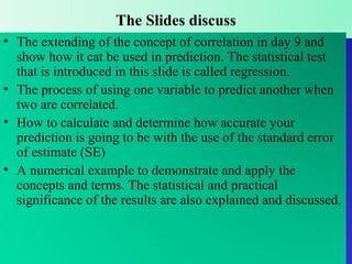
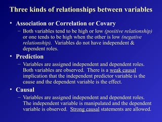
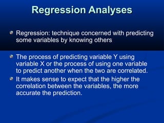
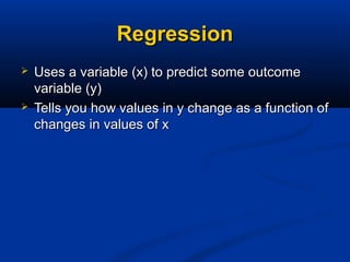
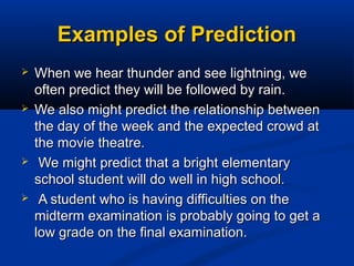
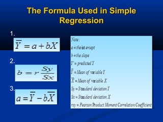
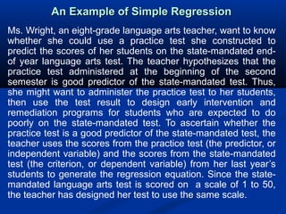
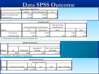
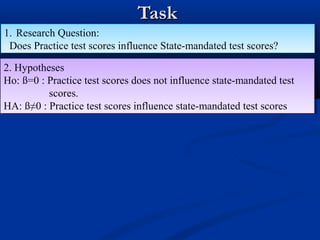
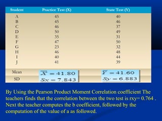
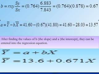
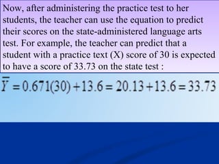
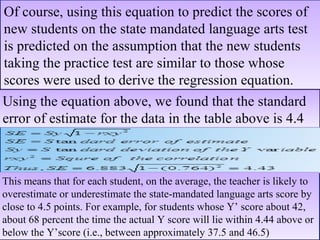
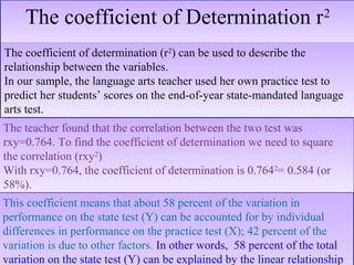
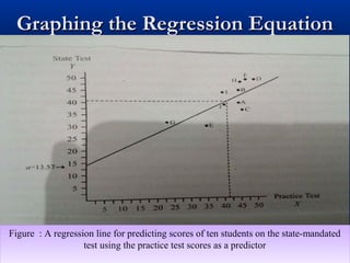
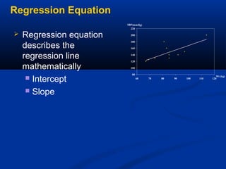
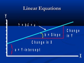
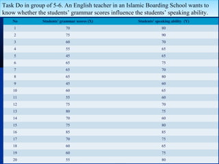
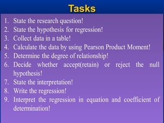
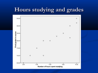
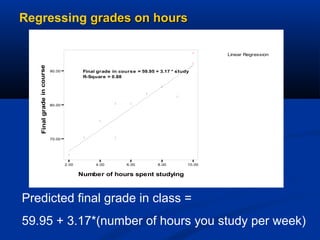
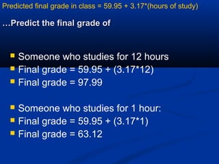
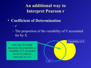
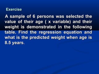
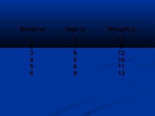
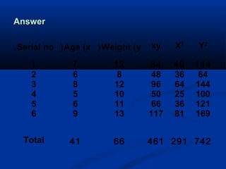
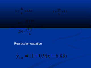
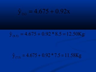
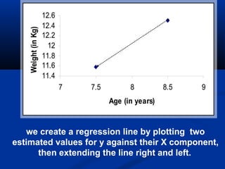
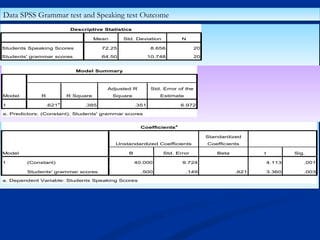
The document discusses the concept of regression and its application in predicting one variable from another when they are correlated. It provides examples, explains how to calculate correlation coefficients and standard errors, and demonstrates the significance of predicting outcomes using regression equations. Additionally, it includes statistical results such as the coefficient of determination and outlines research questions and hypotheses related to educational assessments.

1. Thursday, December 18, 20141

2. The Slides discuss
• The extending of the concept of correlation in day 9 and
show how it cat be used in prediction. The statistical test
that is introduced in this slide is called regression.
• The process of using one variable to predict another when
two are correlated.
• How to calculate and determine how accurate your
prediction is going to be with the use of the standard error
of estimate (SE)
• A numerical example to demonstrate and apply the
concepts and terms. The statistical and practical
significance of the results are also explained and discussed.

3. Three kinds of relationships between variables
• Association or Correlation or Covary
– Both variables tend to be high or low (positive relationship)
or one tends to be high when the other is low (negative
relationship). Variables do not have independent &
dependent roles.
• Prediction
– Variables are assigned independent and dependent roles.
Both variables are observed. There is a weak causal
implication that the independent predictor variable is the
cause and the dependent variable is the effect.
• Causal
– Variables are assigned independent and dependent roles.
The independent variable is manipulated and the dependent
variable is observed. Strong causal statements are allowed.

4. Regression AnalysesRegression Analyses
Regression: technique concerned with predicting
some variables by knowing others
The process of predicting variable Y using
variable X or the process of using one variable
to predict another when the two are correlated.
It makes sense to expect that the higher the
correlation between the variables, the more
accurate the prediction.

5. RegressionRegression
 Uses a variable (x) to predict some outcomeUses a variable (x) to predict some outcome
variable (y)variable (y)
 Tells you how values in y change as a function ofTells you how values in y change as a function of
changes in values of xchanges in values of x

6. Examples of PredictionExamples of Prediction
 When we hear thunder and see lightning, weWhen we hear thunder and see lightning, we
often predict they will be followed by rain.often predict they will be followed by rain.
 We also might predict the relationship betweenWe also might predict the relationship between
the day of the week and the expected crowd atthe day of the week and the expected crowd at
the movie theatre.the movie theatre.
 We might predict that a bright elementaryWe might predict that a bright elementary
school student will do well in high school.school student will do well in high school.
 A student who is having difficulties on theA student who is having difficulties on the
midterm examination is probably going to get amidterm examination is probably going to get a
low grade on the final examination.low grade on the final examination.

7. Correlation and RegressionCorrelation and Regression
 Correlation describes the strength of aCorrelation describes the strength of a linear
relationship between two variables
 Linear means “straight line”
 Regression tells us how to draw the straight line
described by the correlation

8. Simple RegressionSimple Regression
 Prediction is based on the assumption that whenPrediction is based on the assumption that when
two variables are correlated, we can use one oftwo variables are correlated, we can use one of
them to predict the other.them to predict the other.
 The variable used as a predictor is the independent
variable (X). The predicted variable (Y) is called the
criterion variable or dependent variable.
 The technique used for prediction is called
regression.
 When only one variable is used to predict another,
the procedure is called simple regression, and when
two or more variables are used as predictors, the
procedure is called multiple regression.

9. The Formula Used in SimpleThe Formula Used in Simple
RegressionRegression
1.
2.
3.

10. An Example of Simple RegressionAn Example of Simple Regression
Ms. Wright, an eight-grade language arts teacher, want to know
whether she could use a practice test she constructed to
predict the scores of her students on the state-mandated end-
of year language arts test. The teacher hypothesizes that the
practice test administered at the beginning of the second
semester is good predictor of the state-mandated test. Thus,
she might want to administer the practice test to her students,
then use the test result to design early intervention and
remediation programs for students who are expected to do
poorly on the state-mandated test. To ascertain whether the
practice test is a good predictor of the state-mandated test, the
teacher uses the scores from the practice test (the predictor, or
independent variable) and the scores from the state-mandated
test (the criterion, or dependent variable) from her last year’s
students to generate the regression equation. Since the state-
mandated language arts test is scored on a scale of 1 to 50,
the teacher has designed her test to use the same scale.

11. TasksTasks

12. Data SPSS OutcomeData SPSS Outcome
Descriptive Statistics
Mean Std. Deviation N
State-mandated test 41.60 6.883 10
Practice test 41.80 7.843 10
Descriptive Statistics
Mean Std. Deviation N
State-mandated test 41.60 6.883 10
Practice test 41.80 7.843 10
Coefficients
a
Model
Unstandardized Coefficients
Standardized
Coefficients
B Std. Error Beta t Sig.
1 (Constant) 13.572 8.500 1.597 .149
Practice test .671 .200 .764 3.349 .010
a. Dependent Variable: State-mandated test
Coefficients
a
Model
Unstandardized Coefficients
Standardized
Coefficients
B Std. Error Beta t Sig.
1 (Constant) 13.572 8.500 1.597 .149
Practice test .671 .200 .764 3.349 .010
a. Dependent Variable: State-mandated test
Model Summary
Model
Change Statistics
R Square Change
F
Change df1 df2 Sig. F Change
1 .584 11.218 1 8 .010
Model Summary
Model
Change Statistics
R Square Change
F
Change df1 df2 Sig. F Change
1 .584 11.218 1 8 .010

13. TaskTask
1. Research Question:
Does Practice test scores influence State-mandated test scores?
1. Research Question:
Does Practice test scores influence State-mandated test scores?
2. Hypotheses
Ho: ß=0 : Practice test scores does not influence state-mandated test
scores.
HA: ß≠0 : Practice test scores influence state-mandated test scores
2. Hypotheses
Ho: ß=0 : Practice test scores does not influence state-mandated test
scores.
HA: ß≠0 : Practice test scores influence state-mandated test scores

14. Student Practice Test (X) State Test (Y)
A
B
C
D
E
F
G
H
I
J
45
45
46
50
35
47
23
46
40
41
40
46
37
49
31
50
32
48
44
39
Mean
SD
By Using the Pearson Product Moment Correlation coefficient The
teachers finds that the correlation between the two test is rxy= 0.764 .
Next the teacher computes the b coefficient, followed by the
computation of the value of a as followed.

15. After finding the values of b (the slope) and a (the intercept), they can be
entered into the regression equation.
After finding the values of b (the slope) and a (the intercept), they can be
entered into the regression equation.

16. Now, after administering the practice test to her
students, the teacher can use the equation to predict
their scores on the state-administered language arts
test. For example, the teacher can predict that a
student with a practice text (X) score of 30 is expected
to have a score of 33.73 on the state test :
Now, after administering the practice test to her
students, the teacher can use the equation to predict
their scores on the state-administered language arts
test. For example, the teacher can predict that a
student with a practice text (X) score of 30 is expected
to have a score of 33.73 on the state test :

17. Of course, using this equation to predict the scores of
new students on the state mandated language arts test
is predicted on the assumption that the new students
taking the practice test are similar to those whose
scores were used to derive the regression equation.
Of course, using this equation to predict the scores of
new students on the state mandated language arts test
is predicted on the assumption that the new students
taking the practice test are similar to those whose
scores were used to derive the regression equation.
Using the equation above, we found that the standard
error of estimate for the data in the table above is 4.4
Using the equation above, we found that the standard
error of estimate for the data in the table above is 4.4
This means that for each student, on the average, the teacher is likely to
overestimate or underestimate the state-mandated language arts score by
close to 4.5 points. For example, for students whose Y’ score about 42,
about 68 percent the time the actual Y score will lie within 4.44 above or
below the Y’score (i.e., between approximately 37.5 and 46.5)
This means that for each student, on the average, the teacher is likely to
overestimate or underestimate the state-mandated language arts score by
close to 4.5 points. For example, for students whose Y’ score about 42,
about 68 percent the time the actual Y score will lie within 4.44 above or
below the Y’score (i.e., between approximately 37.5 and 46.5)

18. The coefficient of Determination r2The coefficient of Determination r2
The teacher found that the correlation between the two test was
rxy=0.764. To find the coefficient of determination we need to square
the correlation (rxy2
)
With rxy=0.764, the coefficient of determination is 0.7642
= 0.584 (or
58%).
The teacher found that the correlation between the two test was
rxy=0.764. To find the coefficient of determination we need to square
the correlation (rxy2
)
With rxy=0.764, the coefficient of determination is 0.7642
= 0.584 (or
58%).
This coefficient means that about 58 percent of the variation in
performance on the state test (Y) can be accounted for by individual
differences in performance on the practice test (X); 42 percent of the
variation is due to other factors. In other words, 58 percent of the total
variation on the state test (Y) can be explained by the linear relationship
This coefficient means that about 58 percent of the variation in
performance on the state test (Y) can be accounted for by individual
differences in performance on the practice test (X); 42 percent of the
variation is due to other factors. In other words, 58 percent of the total
variation on the state test (Y) can be explained by the linear relationship
The coefficient of determination (r2
) can be used to describe the
relationship between the variables.
In our sample, the language arts teacher used her own practice test to
predict her students’ scores on the end-of-year state-mandated language
arts test.
The coefficient of determination (r2
) can be used to describe the
relationship between the variables.
In our sample, the language arts teacher used her own practice test to
predict her students’ scores on the end-of-year state-mandated language
arts test.

19. Graphing the Regression EquationGraphing the Regression Equation
Figure : A regression line for predicting scores of ten students on the state-mandated
test using the practice test scores as a predictor
Figure : A regression line for predicting scores of ten students on the state-mandated
test using the practice test scores as a predictor

20. Regression Equation
 Regression equation
describes the
regression line
mathematically
 Intercept
 Slope
80
100
120
140
160
180
200
220
60 70 80 90 100 110 120
Wt (kg)
SBP(mmHg)

21. Linear EquationsLinear Equations
Y
Y = b X + a
a = Y - in t e r c e p t
X
C h a n g e
in Y
C h a n g e in X
b = S lo p e
bXayˆ +=

22. Task Do in group of 5-6. An English teacher in an Islamic Boarding School wants to
know whether the students’ grammar scores influence the students’ speaking ability.
Task Do in group of 5-6. An English teacher in an Islamic Boarding School wants to
know whether the students’ grammar scores influence the students’ speaking ability.
No Students’ grammar scores (X) Students’ speaking ability (Y)
1 70 80
2 75 90
3 60 70
4 55 65
5 45 65
6 65 75
7 65 70
8 65 80
9 45 60
10 60 65
11 55 60
12 75 70
13 80 75
14 70 60
15 75 80
16 85 85
17 70 75
18 60 65
19 60 75
20 55 80

23. TasksTasks

24. Hours studying and gradesHours studying and grades

25. Regressing grades on hoursgrades on hours
Linear Regression
2.00 4.00 6.00 8.00 10.00
Number of hours spent studying
70.00
80.00
90.00
Finalgradeincourse












Final grade in course = 59.95 + 3.17 * study
R-Square = 0.88
Predicted final grade in class =
59.95 + 3.17*(number of hours you study per week)

26. Predict the final grade ofPredict the final grade of……
 Someone who studies for 12 hours
 Final grade = 59.95 + (3.17*12)
 Final grade = 97.99
 Someone who studies for 1 hour:
 Final grade = 59.95 + (3.17*1)
 Final grade = 63.12
Predicted final grade in class = 59.95 + 3.17*(hours of study)

27. An additional way to
Interpret Pearson r
• Coefficient of Determination
– r2
– The proportion of the variability of Y accounted
for by X
Variability of Y
This area of overlap
represents the proportion of
variability of Y accounted
for by X (value is
expressed as a %)
X

28. ExerciseExercise
A sample of 6 persons was selected theA sample of 6 persons was selected the
value of their age ( x variable) and theirvalue of their age ( x variable) and their
weight is demonstrated in the followingweight is demonstrated in the following
table. Find the regression equation andtable. Find the regression equation and
what is the predicted weight when age iswhat is the predicted weight when age is
8.5 years8.5 years..

29. Serial no. Age (x( Weight (y(
1
2
3
4
5
6
7
6
8
5
6
9
12
8
12
10
11
13

30. AnswerAnswer
Serial no. Age (x( Weight (y( xy X2
Y2
1
2
3
4
5
6
7
6
8
5
6
9
12
8
12
10
11
13
84
48
96
50
66
117
49
36
64
25
36
81
144
64
144
100
121
169
Total 41 66 461 291 742

31. 6.83
6
41
x == 11
6
66
==y
92.0
6
)41(
291
6
6641
461
2
=
−
×
−
=b
Regression equation
6.83)0.9(x11yˆ (x) −+=

32. 0.92x4.675yˆ (x) +=
12.50Kg8.5*0.924.675yˆ (8.5) =+=
Kg58.117.5*0.924.675yˆ (7.5) =+=

33. 11.4
11.6
11.8
12
12.2
12.4
12.6
7 7.5 8 8.5 9
Age (in years)
Weight(inKg)
we create a regression line by plotting two
estimated values for y against their X component,
then extending the line right and left.

34. Data SPSS Grammar test and Speaking test OutcomeData SPSS Grammar test and Speaking test Outcome
Descriptive Statistics
Mean Std. Deviation N
Students Speaking Scores 72.25 8.656 20
Students' grammar scores 64.50 10.748 20
Descriptive Statistics
Mean Std. Deviation N
Students Speaking Scores 72.25 8.656 20
Students' grammar scores 64.50 10.748 20
Model Summary
Model R R Square
Adjusted R
Square
Std. Error of the
Estimate
1 .621
a
.385 .351 6.972
a. Predictors: (Constant), Students' grammar scores
Model Summary
Model R R Square
Adjusted R
Square
Std. Error of the
Estimate
1 .621
a
.385 .351 6.972
a. Predictors: (Constant), Students' grammar scores
Coefficients
a
Model
Unstandardized Coefficients
Standardized
Coefficients
B Std. Error Beta t Sig.
1 (Constant) 40.000 9.724 4.113 .001
Students' grammar scores .500 .149 .621 3.360 .003
a. Dependent Variable: Students Speaking Scores
Coefficients
a
Model
Unstandardized Coefficients
Standardized
Coefficients
B Std. Error Beta t Sig.
1 (Constant) 40.000 9.724 4.113 .001
Students' grammar scores .500 .149 .621 3.360 .003
a. Dependent Variable: Students Speaking Scores

35. ReferencesReferencesMain Sources
Coolidge, F. L.2000. Statistics: A gentle introduction. London: Sage.
Kranzler, G & Moursund, J .1999. Statistics for the terrified. (2nd ed.). Upper Saddle
River, NJ: Prentice Hall.
Butler Christopher.1985. Statistics in Linguistics. Oxford: Basil Blackwell.
Hatch Evelyn & Hossein Farhady.1982. Research design and Statistics for Applied Linguistics.
Massachusetts: Newbury House Publishers, Inc.
Ravid Ruth.2011. Practical Statistics for Educators, fourth Ed. New York: Rowman &
Littlefield Publisher, Inc.
Quirk Thomas. 2012. Excel 2010 for Educational and Psychological Statistics: A Guide
to Solving Practical Problem. New York: Springer.
Other relevant sources
Agresi A, & B. Finlay.1986. Statistical methods for the social sciences. San Francisco,
CA: Dellen Publishing Company.
Bachman, L.F. 2004. Statistical Analysis for Language Assessment. New York: Cambridge University
Press.
Field, A. (2005). Discovering statistics using SPSS (2nd ed.). London: Sage.
Moore, D. S. (2000). The basic practice of statistics (2nd ed.). New York: W. H.
Freeman and Company.