Slideset Simple Linear Regression models.ppt

Linear correlation and linear
regression

Continuous outcome (means)
Outcome
Variable
Are the observations independent or correlated?
Alternatives if the normality
assumption is violated (and
small sample size):
independent correlated
Continuous
(e.g. pain
scale,
cognitive
function)
Ttest: compares means
between two independent
groups
ANOVA: compares means
between more than two
independent groups
Pearson’s correlation
coefficient (linear
correlation): shows linear
correlation between two
continuous variables
Linear regression:
multivariate regression technique
used when the outcome is
continuous; gives slopes
Paired ttest: compares means
between two related groups (e.g.,
the same subjects before and
after)
Repeated-measures
ANOVA: compares changes
over time in the means of two or
more groups (repeated
measurements)
Mixed models/GEE
modeling: multivariate
regression techniques to compare
changes over time between two
or more groups; gives rate of
change over time
Non-parametric statistics
Wilcoxon sign-rank test:
non-parametric alternative to the
paired ttest
Wilcoxon sum-rank test
(=Mann-Whitney U test): non-
parametric alternative to the ttest
Kruskal-Wallis test: non-
parametric alternative to ANOVA
Spearman rank correlation
coefficient: non-parametric
alternative to Pearson’s correlation
coefficient

Recall: Covariance
1
)
)(
(
)
,
(
cov 1






n
Y
y
X
x
y
x
n
i
i
i

cov(X,Y) > 0 X and Y are positively correlated
cov(X,Y) < 0 X and Y are inversely correlated
cov(X,Y) = 0 X and Y are independent
Interpreting Covariance

Correlation coefficient
 Pearson’s Correlation Coefficient is
standardized covariance (unitless):
y
x
y
x
ariance
r
var
var
)
,
(
cov


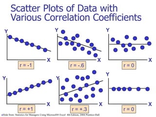
Correlation
 Measures the relative strength of the linear
relationship between two variables
 Unit-less
 Ranges between –1 and 1
 The closer to –1, the stronger the negative linear
relationship
 The closer to 1, the stronger the positive linear
relationship
 The closer to 0, the weaker any positive linear
relationship

Scatter Plots of Data with
Various Correlation Coefficients
Y
X
Y
X
Y
X
Y
X
Y
X
r = -1 r = -.6 r = 0
r = +.3
r = +1
Y
X
r = 0
Slide from: Statistics for Managers Using Microsoft® Excel 4th Edition, 2004 Prentice-Hall

Y
X
Y
X
Y
Y
X
X
Linear relationships Curvilinear relationships
Linear Correlation

Y
X
Y
X
Y
Y
X
X
Strong relationships Weak relationships
Linear Correlation

Linear Correlation
Y
X
Y
X
No relationship

Calculating by hand…
1
)
(
1
)
(
1
)
)(
(
var
var
)
,
(
cov
ˆ
1
2
1
2
1















n
y
y
n
x
x
n
y
y
x
x
y
x
y
x
ariance
r
n
i
i
n
i
i
n
i
i
i

Simpler calculation formula…
y
x
xy
n
i
i
n
i
i
n
i
i
i
n
i
i
n
i
i
n
i
i
i
SS
SS
SS
y
y
x
x
y
y
x
x
n
y
y
n
x
x
n
y
y
x
x
r


























1
2
1
2
1
1
2
1
2
1
)
(
)
(
)
)(
(
1
)
(
1
)
(
1
)
)(
(
ˆ
y
x
xy
SS
SS
SS
r 
ˆ
Numerator of
covariance
Numerators of
variance

Distribution of the
correlation coefficient:
*note, like a proportion, the variance of the correlation coefficient depends
on the correlation coefficient itselfsubstitute in estimated r
2
1
)
ˆ
(
2



n
r
r
SE
The sample correlation coefficient follows a T-distribution with
n-2 degrees of freedom (since you have to estimate the
standard error).

Linear regression
In correlation, the two variables are treated as equals. In regression, one
variable is considered independent (=predictor) variable (X) and the other the
dependent (=outcome) variable Y.

What is “Linear”?
 Remember this:
 Y=mX+B?
B
m

What’s Slope?
A slope of 2 means that every 1-unit change in X
yields a 2-unit change in Y.

Prediction
If you know something about X, this knowledge helps you
predict something about Y. (Sound familiar?…sound
like conditional probabilities?)

Regression equation…
i
i
i x
x
y
E 
 

)
/
(
Expected value of y at a given level of x=

Predicted value for an
individual…
yi=  + *xi + random errori
Follows a normal
distribution
Fixed –
exactly
on the
line

Assumptions (or the fine print)
 Linear regression assumes that…
 1. The relationship between X and Y is linear
 2. Y is distributed normally at each value of X
 3. The variance of Y at every value of X is the
same (homogeneity of variances)
 4. The observations are independent

The standard error of Y given X is the average variability around the
regression line at any given value of X. It is assumed to be equal at
all values of X.
Sy/x
Sy/x
Sy/x
Sy/x
Sy/x
Sy/x

C A
B
A
yi
x
y
yi
C
B
*Least squares estimation
gave us the line (β) that
minimized C2

 
 i
i x
ŷ
y
A2 B2 C2
SStotal
Total squared distance of
observations from naïve mean
of y
Total variation
SSreg
Distance from regression line to naïve mean of y
Variability due to x (regression)
SSresidual
Variance around the regression line
Additional variability not explained
by x—what least squares method aims
to minimize

  
 





n
i
i
i
n
i
n
i
i
i y
y
y
y
y
y
1
2
1 1
2
2
)
ˆ
(
)
ˆ
(
)
(
Regression Picture
R2=SSreg/SStotal

Recall example: cognitive
function and vitamin D
 Hypothetical data loosely based on [1];
cross-sectional study of 100 middle-
aged and older European men.
 Cognitive function is measured by the Digit
Symbol Substitution Test (DSST).
1. Lee DM, Tajar A, Ulubaev A, et al. Association between 25-hydroxyvitamin D levels and cognitive performance in middle-aged
and older European men. J Neurol Neurosurg Psychiatry. 2009 Jul;80(7):722-9.

Distribution of vitamin D
Mean= 63 nmol/L
Standard deviation = 33 nmol/L

Distribution of DSST
Normally distributed
Mean = 28 points
Standard deviation = 10 points

Four hypothetical datasets
 I generated four hypothetical datasets,
with increasing TRUE slopes (between
vit D and DSST):
 0
 0.5 points per 10 nmol/L

Dataset 3: weak to moderate
relationship

Dataset 4: moderate
relationship

The “Best fit” line
Regression
equation:
E(Yi) = 28 + 0*vit
Di (in 10 nmol/L)

Note how the line is
a little deceptive; it
draws your eye,
making the
relationship appear
stronger than it
really is!
Regression
equation:
E(Yi) = 26 + 0.5*vit
Di (in 10 nmol/L)

Regression equation:
E(Yi) = 22 + 1.0*vit
Di (in 10 nmol/L)

Regression equation:
E(Yi) = 20 + 1.5*vit Di
(in 10 nmol/L)
Note: all the lines go
through the point
(63, 28)!

Estimating the intercept and
slope: least squares estimation
** Least Squares Estimation
A little calculus….
What are we trying to estimate? β, the slope, from
What’s the constraint? We are trying to minimize the squared distance (hence the “least squares”) between the
observations themselves and the predicted values , or (also called the “residuals”, or left-over unexplained variability)
Differencei = yi – (βx + α) Differencei
2 = (yi – (βx + α)) 2
Find the β that gives the minimum sum of the squared differences. How do you maximize a function? Take the
derivative; set it equal to zero; and solve. Typical max/min problem from calculus….
From here takes a little math trickery to solve for β…
...
0
))
(
(
2
))
)(
(
(
2
))
(
(
1
2
1
1
2
















n
i
i
i
i
i
n
i
i
i
i
n
i
i
i
x
x
x
y
x
x
y
x
y
d
d








Resulting formulas…
Slope (beta coefficient) =
)
(
)
,
(
ˆ
x
Var
y
x
Cov


)
,
( y
x
x
ˆ
-
y
ˆ
:
Calculate 
 
Intercept=
Regression line always goes through the point:

Relationship with correlation
y
x
SD
SD
r ̂
ˆ 
In correlation, the two variables are treated as equals. In regression, one variable is considered
independent (=predictor) variable (X) and the other the dependent (=outcome) variable Y.

Example: dataset 4
y
x
SS
SS
̂
SDx = 33 nmol/L
SDy= 10 points
Cov(X,Y) = 163
points*nmol/L
Beta = 163/332 = 0.15
points per nmol/L
= 1.5 points per 10
nmol/L
r = 163/(10*33) = 0.49
Or
r = 0.15 * (33/10) = 0.49

Significance testing…
Slope
Distribution of slope ~ Tn-2(β,s.e.( ))

ˆ
H0: β1 = 0 (no linear relationship)
H1: β1  0 (linear relationship does exist)
)
ˆ
.(
.
0
ˆ


e
s

Tn-2=

Formula for the standard error of
beta (you will not have to calculate
by hand!):
i
i
n
i
i
x
y
x
x

 ˆ
ˆ
ˆ
and
)
(
SS
where
1
2
x



 

x
x
y
x
n
i
i
i
SS
s
SS
n
y
y
s
2
/
1
2
ˆ
2
)
ˆ
(








Example: dataset 4
 Standard error (beta) = 0.03
 T98 = 0.15/0.03 = 5, p<.0001
 95% Confidence interval = 0.09 to 0.21

Residual Analysis: check
assumptions
 The residual for observation i, ei, is the difference
between its observed and predicted value
 Check the assumptions of regression by examining the
residuals
 Examine for linearity assumption
 Examine for constant variance for all levels of X
(homoscedasticity)
 Evaluate normal distribution assumption
 Evaluate independence assumption
 Graphical Analysis of Residuals
 Can plot residuals vs. X
i
i
i Y
Y
e ˆ



Predicted values…
i
i x
y 5
.
1
20
ˆ 

For Vitamin D = 95 nmol/L (or 9.5 in 10 nmol/L):
34
)
5
.
9
(
5
.
1
20
ˆ 


i
y

Residual =
observed - predicted
14
ˆ
34
ˆ
48




i
i
i
i
y
y
y
y
X=95
nmol/L
34

Residual Analysis for
Linearity
Not Linear Linear

x
residuals
x
Y
x
Y
x
residuals

Homoscedasticity
Non-constant variance  Constant variance
x x
Y
x x
Y
residuals
residuals

Independence
Not Independent
Independent
X
X
residuals
residuals
X
residuals


Multiple linear regression…
 What if age is a confounder here?
 Older men have lower vitamin D
 Older men have poorer cognition
 “Adjust” for age by putting age in the
model:
 DSST score = intercept + slope1xvitamin D
+ slope2 xage

2 predictors: age and vit D…

Fit a plane rather than a line…
On the plane, the
slope for vitamin
D is the same at
every age; thus,
the slope for
vitamin D
represents the
effect of vitamin
D when age is
held constant.

Equation of the “Best fit”
plane…
 DSST score = 53 + 0.0039xvitamin D
(in 10 nmol/L) - 0.46 xage (in years)
 P-value for vitamin D >>.05
 P-value for age <.0001
 Thus, relationship with vitamin D was
due to confounding by age!

Multiple Linear Regression
 More than one predictor…
E(y)=  + 1*X + 2 *W + 3 *Z…
Each regression coefficient is the amount of
change in the outcome variable that would be
expected per one-unit change of the
predictor, if all other variables in the model
were held constant.

Functions of multivariate
analysis:
 Control for confounders
 Test for interactions between predictors
(effect modification)
 Improve predictions

A ttest is linear regression!
 Divide vitamin D into two groups:
 Insufficient vitamin D (<50 nmol/L)
 Sufficient vitamin D (>=50 nmol/L), reference
group
 We can evaluate these data with a ttest or a
linear regression…
0008
.
;
46
.
3
46
8
.
10
54
8
.
10
5
.
7
5
.
32
40
2
2
98 




 p
T

As a linear regression…
Parameter ````````````````Standard
Variable Estimate Error t Value Pr > |t|
Intercept 40.07407 1.47511 27.17 <.0001
insuff -7.53060 2.17493 -3.46 0.0008
Intercept
represents the
mean value in
the sufficient
group.
Slope represents
the difference in
means between the
groups. Difference
is significant.

ANOVA is linear regression!
 Divide vitamin D into three groups:
 Deficient (<25 nmol/L)
 Insufficient (>=25 and <50 nmol/L)
 Sufficient (>=50 nmol/L), reference group
DSST=  (=value for sufficient) + insufficient*(1
if insufficient) + 2 *(1 if deficient)
This is called “dummy coding”—where multiple
binary variables are created to represent
being in each category (or not) of a
categorical variable

The picture…
Sufficient vs.
Insufficient
Sufficient vs.
Deficient

Results…
Parameter Estimates
Parameter Standard
Variable DF Estimate Error t Value Pr > |t|
Intercept 1 40.07407 1.47817 27.11 <.0001
deficient 1 -9.87407 3.73950 -2.64 0.0096
insufficient 1 -6.87963 2.33719 -2.94 0.0041
 Interpretation:
 The deficient group has a mean DSST 9.87 points
lower than the reference (sufficient) group.
 The insufficient group has a mean DSST 6.87
points lower than the reference (sufficient) group.

Other types of multivariate
regression
 Multiple linear regression is for normally
distributed outcomes
 Logistic regression is for binary outcomes
 Cox proportional hazards regression is used when
time-to-event is the outcome

Common multivariate regression models.
Outcome
(dependent
variable)
Example
outcome
variable
Appropriate
multivariate
regression
model
Example equation What do the coefficients give
you?
Continuous Blood
pressure
Linear
regression
blood pressure (mmHg) =
 + salt*salt consumption (tsp/day) +
age*age (years) + smoker*ever
smoker (yes=1/no=0)
slopes—tells you how much
the outcome variable
increases for every 1-unit
increase in each predictor.
Binary High blood
pressure
(yes/no)
Logistic
regression
ln (odds of high blood pressure) =
smoker (yes=1/no=0)
odds ratios—tells you how
much the odds of the
outcome increase for every
1-unit increase in each
predictor.
Time-to-event Time-to-
death
Cox regression ln (rate of death) =
smoker (yes=1/no=0)
hazard ratios—tells you how
much the rate of the outcome
increases for every 1-unit
increase in each predictor.

Multivariate regression pitfalls
 Multi-collinearity
 Residual confounding
 Overfitting

Multicollinearity
 Multicollinearity arises when two variables that
measure the same thing or similar things (e.g.,
weight and BMI) are both included in a multiple
regression model; they will, in effect, cancel each
other out and generally destroy your model.
 Model building and diagnostics are tricky
business!

Residual confounding
 You cannot completely wipe out
confounding simply by adjusting for
variables in multiple regression unless
variables are measured with zero error
(which is usually impossible).
 Example: meat eating and mortality

Men who eat a lot of meat are
unhealthier for many reasons!
Sinha R, Cross AJ, Graubard BI, Leitzmann MF, Schatzkin A. Meat intake and mortality: a prospective study of over half a million people. Arch
Intern Med 2009;169:562-71

Mortality risks…
Sinha R, Cross AJ, Graubard BI, Leitzmann MF, Schatzkin A. Meat intake and mortality: a prospective study of over half a million people. Arch
Intern Med 2009;169:562-71

Overfitting
 In multivariate modeling, you can get
highly significant but meaningless
results if you put too many predictors in
the model.
 The model is fit perfectly to the quirks
of your particular sample, but has no
predictive ability in a new sample.

Overfitting: class data
example
 I asked SAS to automatically find
predictors of optimism in our class
dataset. Here’s the resulting linear
regression model:
Parameter Standard
Variable Estimate Error Type II SS F Value Pr > F
Intercept 11.80175 2.98341 11.96067 15.65 0.0019
exercise -0.29106 0.09798 6.74569 8.83 0.0117
sleep -1.91592 0.39494 17.98818 23.53 0.0004
obama 1.73993 0.24352 39.01944 51.05 <.0001
Clinton -0.83128 0.17066 18.13489 23.73 0.0004
mathLove 0.45653 0.10668 13.99925 18.32 0.0011
Exercise, sleep, and high ratings for Clinton are negatively related to optimism (highly
significant!) and high ratings for Obama and high love of math are positively related to
optimism (highly significant!).

If something seems to good to
be true…
Clinton, univariate:
Parameter Standard
Variable Label DF Estimate Error t Value Pr > |t|
Intercept Intercept 1 5.43688 2.13476 2.55 0.0188
Clinton Clinton 1 0.24973 0.27111 0.92 0.3675
Sleep, Univariate:
Parameter Standard
sleep sleep 1 -0.14484 0.65451 -0.22 0.8270
Exercise, Univariate:
Parameter Standard
Intercept Intercept 1 6.65189 0.89153 7.46 <.0001
exercise exercise 1 0.19161 0.20709 0.93 0.3658

More univariate models…
Obama, Univariate:
Parameter Standard
obama obama 1 0.87276 0.31973 2.73 0.0126
Love of Math, univariate:
Parameter Standard
mathLove mathLove 1 0.59459 0.19225 3.09 0.0055
Compare
with
multivariate
result;
p<.0001
Compare
with
multivariate
result;
p=.0011

Overfitting
Pure noise variables still produce good R2 values if the model is
overfitted. The distribution of R2 values from a series of
simulated regression models containing only noise variables.
(Figure 1 from: Babyak, MA. What You See May Not Be What You Get: A Brief, Nontechnical Introduction
to Overfitting in Regression-Type Models. Psychosomatic Medicine 66:411-421 (2004).)
Rule of thumb: You need at
least 10 subjects for each
additional predictor
variable in the multivariate
regression model.

Review of statistical tests
The following table gives the appropriate
choice of a statistical test or measure of
association for various types of data (outcome
variables and predictor variables) by study
design.
Continuous outcome
Binary predictor
Continuous predictors
e.g., blood pressure= pounds + age + treatment (1/0)

Types of variables to be analyzed
Statistical procedure
or measure of association
Predictor variable/s Outcome variable
Cross-sectional/case-control studies
Categorical (>2 groups) Continuous ANOVA
Continuous Continuous Simple linear regression
Multivariate
(categorical and
continuous)
Continuous Multiple linear regression
Categorical Categorical
Chi-square test (or Fisher’s
exact)
Binary Binary Odds ratio, risk ratio
Multivariate Binary Logistic regression
Cohort Studies/Clinical Trials
Binary Binary Risk ratio
Categorical Time-to-event Kaplan-Meier/ log-rank test
Multivariate Time-to-event
Cox-proportional hazards
regression, hazard ratio
Binary (two groups) Continuous T-test
Binary Ranks/ordinal Wilcoxon rank-sum test
Categorical Continuous Repeated measures ANOVA
Multivariate Continuous Mixed models; GEE modeling

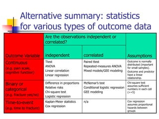
Alternative summary: statistics
for various types of outcome data
Outcome Variable
Are the observations independent or
correlated?
Assumptions
Continuous
(e.g. pain scale,
cognitive function)
Ttest
ANOVA
Linear correlation
Linear regression
Paired ttest
Repeated-measures ANOVA
Mixed models/GEE modeling
Outcome is normally
distributed (important
for small samples).
Outcome and predictor
have a linear
relationship.
Binary or
categorical
(e.g. fracture yes/no)
Difference in proportions
Relative risks
Chi-square test
Logistic regression
McNemar’s test
Conditional logistic regression
GEE modeling
Chi-square test
assumes sufficient
numbers in each cell
(>=5)
Time-to-event
(e.g. time to fracture)
Kaplan-Meier statistics
Cox regression
n/a Cox regression
assumes proportional
hazards between
groups

Continuous outcome (means);
HRP 259/HRP 262
Outcome
Variable
Are the observations independent or correlated?
Alternatives if the normality
assumption is violated (and
small sample size):
Continuous
(e.g. pain
scale,
cognitive
function)
Ttest: compares means
between two independent
groups
ANOVA: compares means
between more than two
independent groups
Pearson’s correlation
coefficient (linear
correlation): shows linear
correlation between two
continuous variables
Linear regression:
multivariate regression technique
used when the outcome is
continuous; gives slopes
Paired ttest: compares means
between two related groups (e.g.,
the same subjects before and
after)
Repeated-measures
ANOVA: compares changes
over time in the means of two or
more groups (repeated
measurements)
Mixed models/GEE
modeling: multivariate
regression techniques to compare
changes over time between two
or more groups; gives rate of
change over time
Non-parametric statistics
Wilcoxon sign-rank test:
non-parametric alternative to the
paired ttest
Wilcoxon sum-rank test
(=Mann-Whitney U test): non-
parametric alternative to the ttest
Kruskal-Wallis test: non-
parametric alternative to ANOVA
Spearman rank correlation
coefficient: non-parametric
alternative to Pearson’s correlation
coefficient

Binary or categorical outcomes
(proportions); HRP 259/HRP 261
Outcome
Variable
Are the observations correlated? Alternative to the chi-
square test if sparse
cells:
Binary or
categorical
(e.g.
fracture,
yes/no)
Chi-square test:
compares proportions between
two or more groups
Relative risks: odds ratios
or risk ratios
Logistic regression:
multivariate technique used
when outcome is binary; gives
multivariate-adjusted odds
ratios
McNemar’s chi-square test:
compares binary outcome between
correlated groups (e.g., before and
after)
Conditional logistic
regression: multivariate
regression technique for a binary
outcome when groups are
correlated (e.g., matched data)
GEE modeling: multivariate
regression technique for a binary
outcome when groups are
correlated (e.g., repeated measures)
Fisher’s exact test: compares
proportions between independent
groups when there are sparse data
(some cells <5).
McNemar’s exact test:
compares proportions between
correlated groups when there are
sparse data (some cells <5).

Time-to-event outcome
(survival data); HRP 262
Outcome
Variable
Are the observation groups independent or correlated? Modifications to
Cox regression
if proportional-
hazards is
violated:
Time-to-
event (e.g.,
time to
fracture)
Kaplan-Meier statistics: estimates survival functions for
each group (usually displayed graphically); compares survival
functions with log-rank test
Cox regression: Multivariate technique for time-to-event data;
gives multivariate-adjusted hazard ratios
n/a (already over
time)
Time-dependent
predictors or time-
dependent hazard
ratios (tricky!)

Slideset Simple Linear Regression models.ppt

Recommended

Recommended

More Related Content

Similar to Slideset Simple Linear Regression models.ppt

Similar to Slideset Simple Linear Regression models.ppt (20)

Recently uploaded

Recently uploaded (20)

Slideset Simple Linear Regression models.ppt