The document outlines various forecasting techniques critical for achieving business objectives, emphasizing both quantitative and qualitative methods. It details specific models like time series and causal models, along with their applications in economic and demand forecasting, as well as methods for measuring forecast accuracy. Additionally, it discusses innovative collaborative approaches like CPFR (Collaborative Planning, Forecasting, and Replenishment) to enhance supply chain efficiencies.

1. Forecasting Techniques Interventions required to meet business objectives Anand Subramaniam

2. “ An ardent supporter of the hometown team should go to a game prepared to take offense, no matter what happens.” - Robert Benchley

3. Highlights Forecasting Methods Quantitative Methods – Examples Forecast Accuracy / Error Reduction Integrate – Sales Forecast / Production CPFR - Collaborative Planning, Forecasting and Replenishment

4. Forecasting Methods

5. Planning Levels

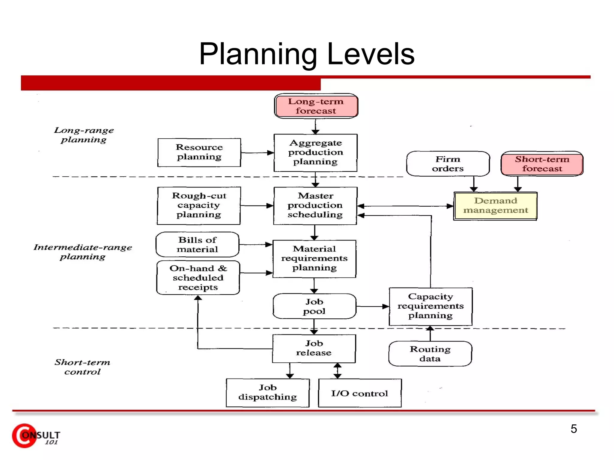
6. Forecast Horizon Trend Exploration Graphical Methods Exponential Smoothing Purchasing Detailed Job Scheduling 1 day ~ I year Short Time Series Regression Staffing Plans Aggregate Production Plan 1 season ~ 2 years Intermediate Economic Demographic Market Information Technology Facility Planning Capacity Planning Product Planning > 5 years Long Methods Applications Horizon Range

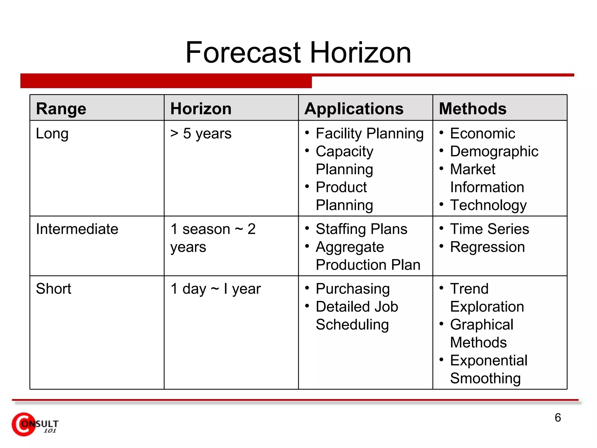
7. Major Areas of Forecasting Economic Forecasting Predicts what the general business conditions will be in the future (Eg. Inflation rates, Gross National Product, Tax, Level of employment) Technology Forecasting Predicts the probability and / or possible future developments in technology (Eg. Competitive advantage or firm’s competitors incorporate into their products and processes) Demand Forecasting Predicts the quantity and timing of demand for a firm’s products

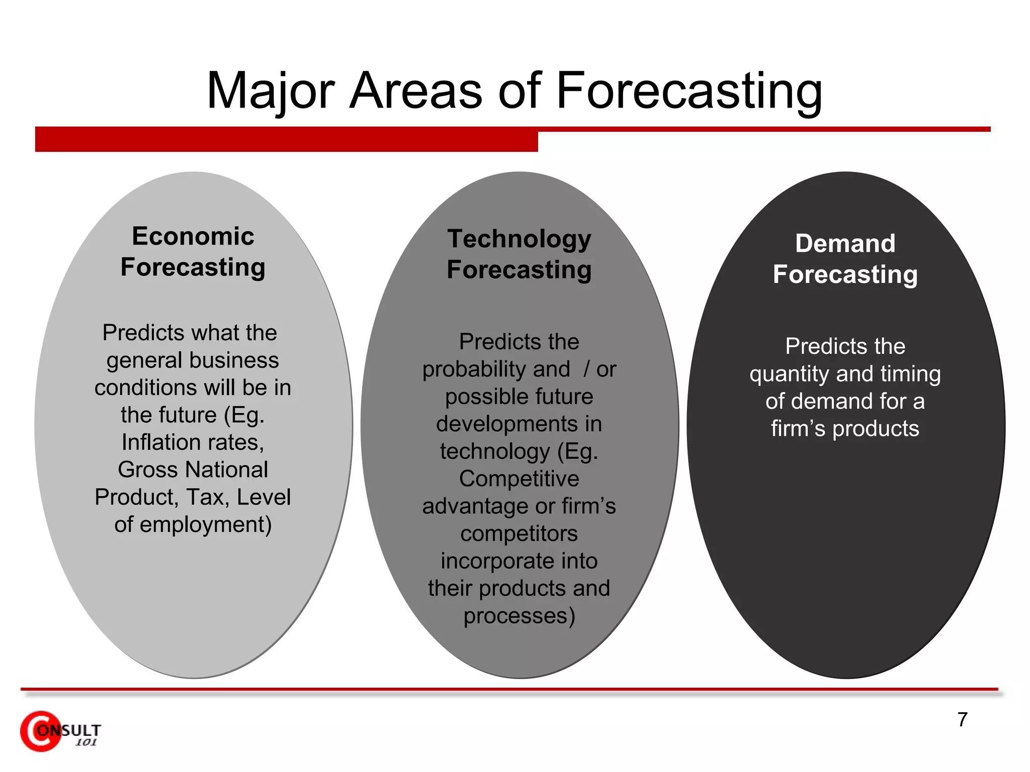
8. Forecasting Methods Subjective Approach (Qualitative in nature and usually based on the opinions of people) Objective Approach (Quantitative / Mathematical formulations - statistical forecasting)

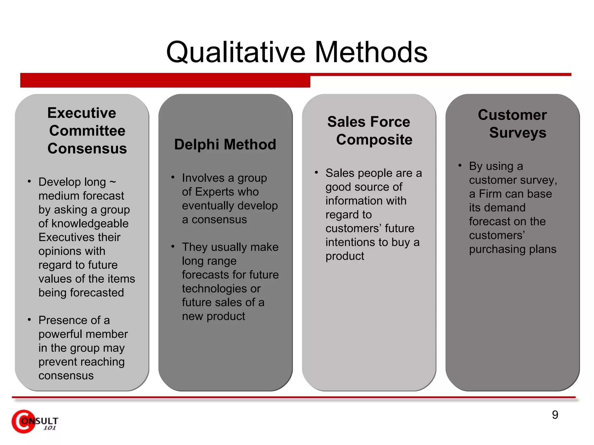
9. Qualitative Methods Executive Committee Consensus Develop long ~ medium forecast by asking a group of knowledgeable Executives their opinions with regard to future values of the items being forecasted Presence of a powerful member in the group may prevent reaching consensus Delphi Method Involves a group of Experts who eventually develop a consensus They usually make long range forecasts for future technologies or future sales of a new product Sales Force Composite Sales people are a good source of information with regard to customers’ future intentions to buy a product Customer Surveys By using a customer survey, a Firm can base its demand forecast on the customers’ purchasing plans

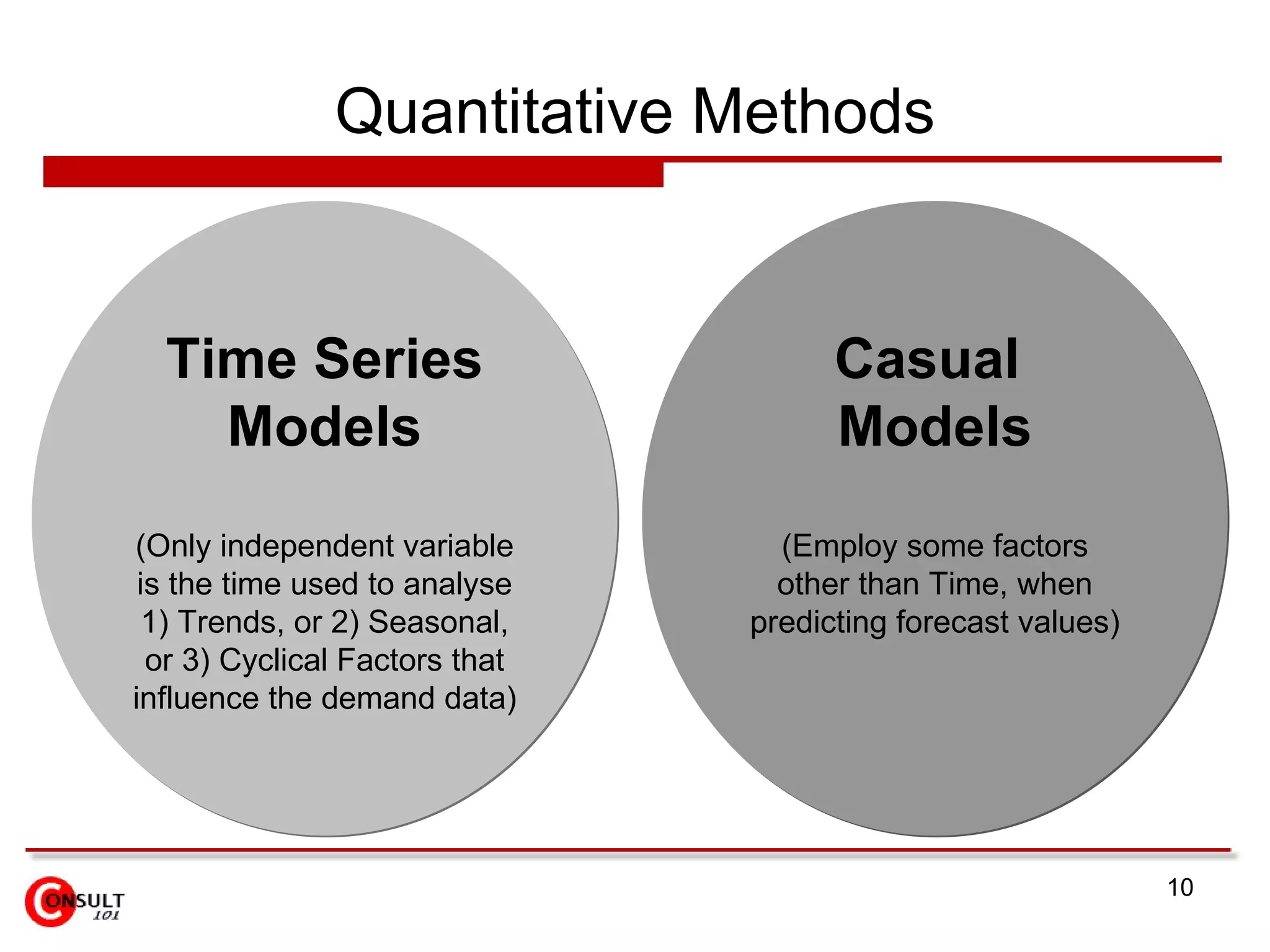
10. Quantitative Methods Time Series Models (Only independent variable is the time used to analyse 1) Trends, or 2) Seasonal, or 3) Cyclical Factors that influence the demand data) Casual Models (Employ some factors other than Time, when predicting forecast values)

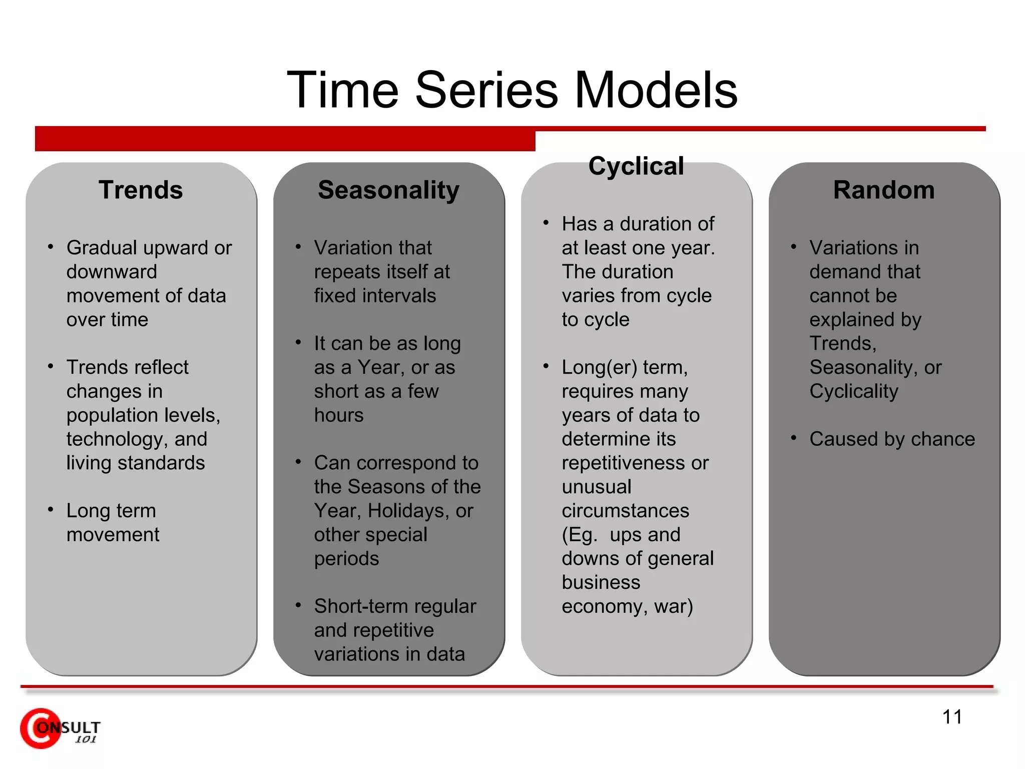
11. Time Series Models Trends Gradual upward or downward movement of data over time Trends reflect changes in population levels, technology, and living standards Long term movement Seasonality Variation that repeats itself at fixed intervals It can be as long as a Year, or as short as a few hours Can correspond to the Seasons of the Year, Holidays, or other special periods Short-term regular and repetitive variations in data Cyclical Has a duration of at least one year. The duration varies from cycle to cycle Long(er) term, requires many years of data to determine its repetitiveness or unusual circumstances (Eg. ups and downs of general business economy, war) Random Variations in demand that cannot be explained by Trends, Seasonality, or Cyclicality Caused by chance

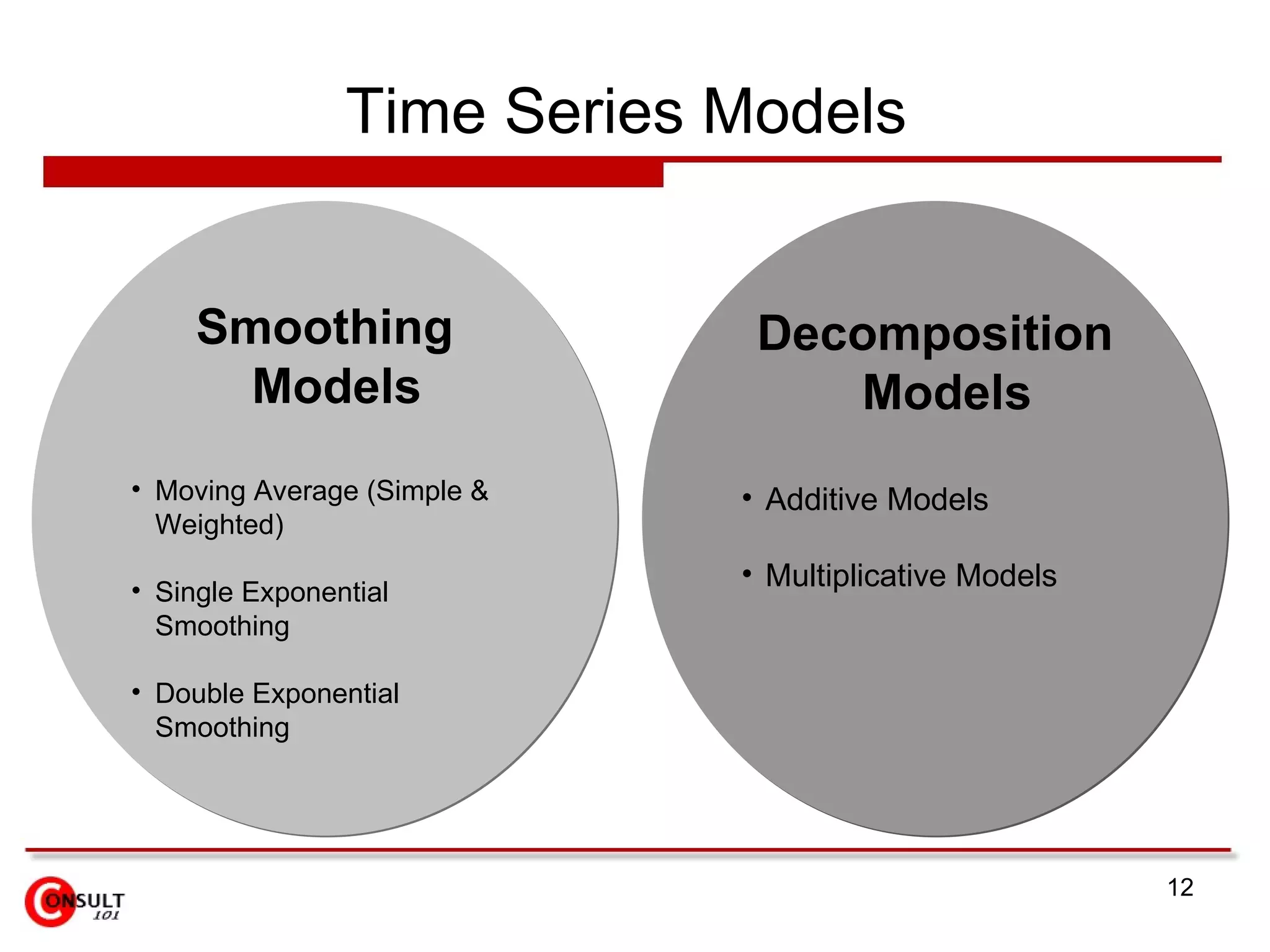
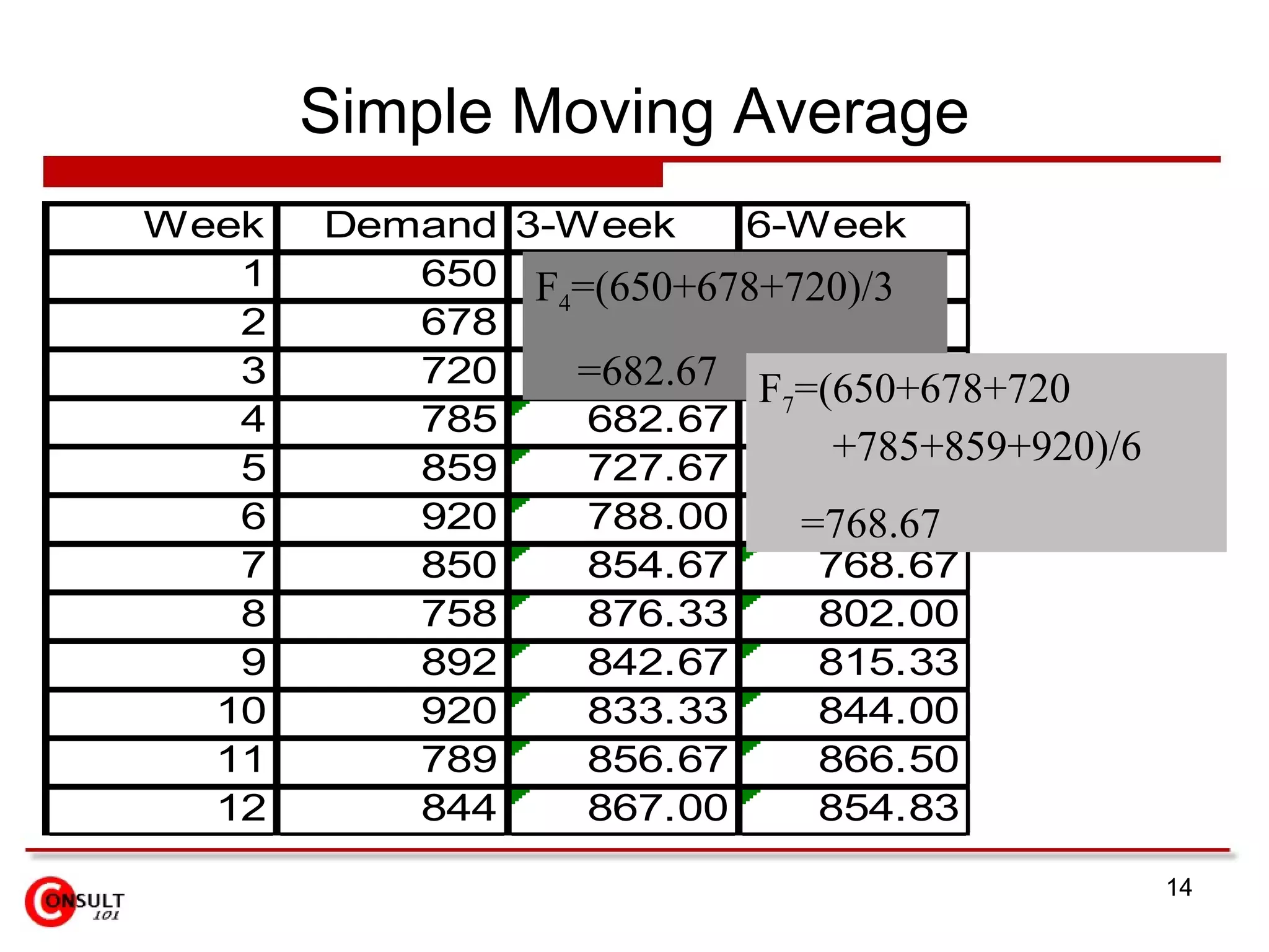
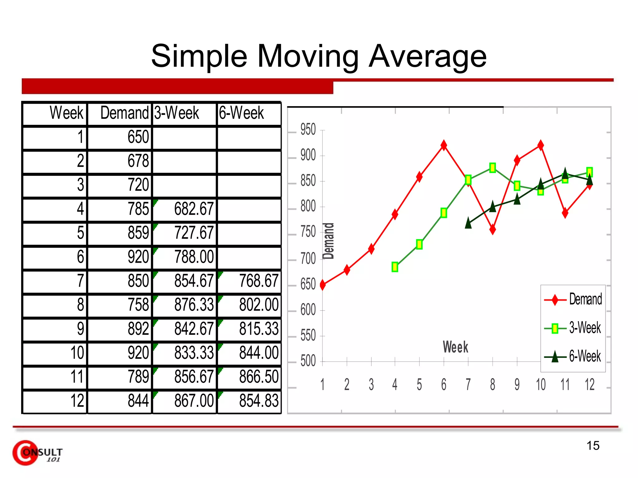
12. Time Series Models Smoothing Models Moving Average (Simple & Weighted) Single Exponential Smoothing Double Exponential Smoothing Decomposition Models Additive Models Multiplicative Models

13. Quantitative Methods - Examples

14. Simple Moving Average F 4 =(650+678+720)/3 =682.67 F 7 =(650+678+720 +785+859+920)/6 =768.67

15. Simple Moving Average

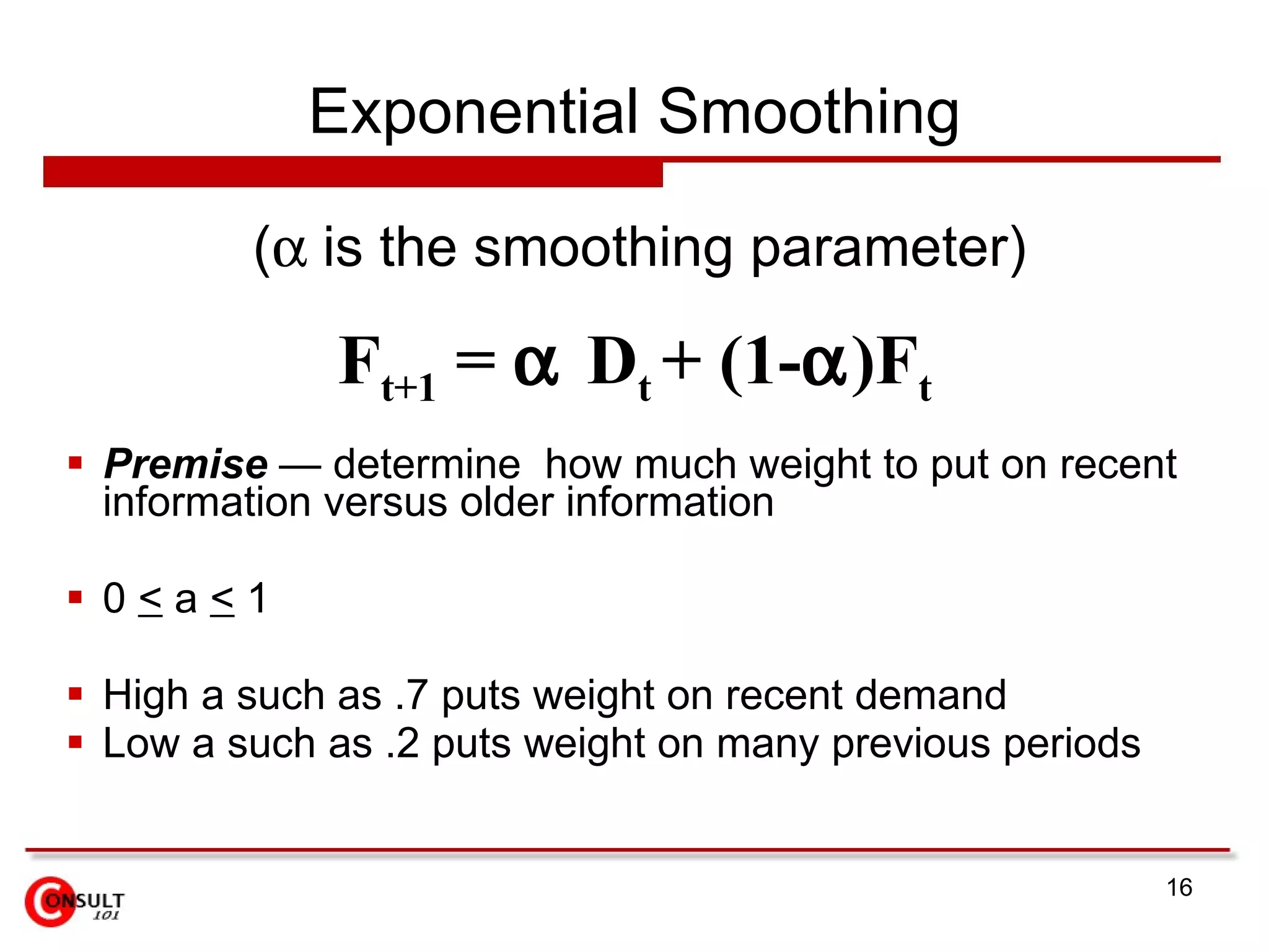
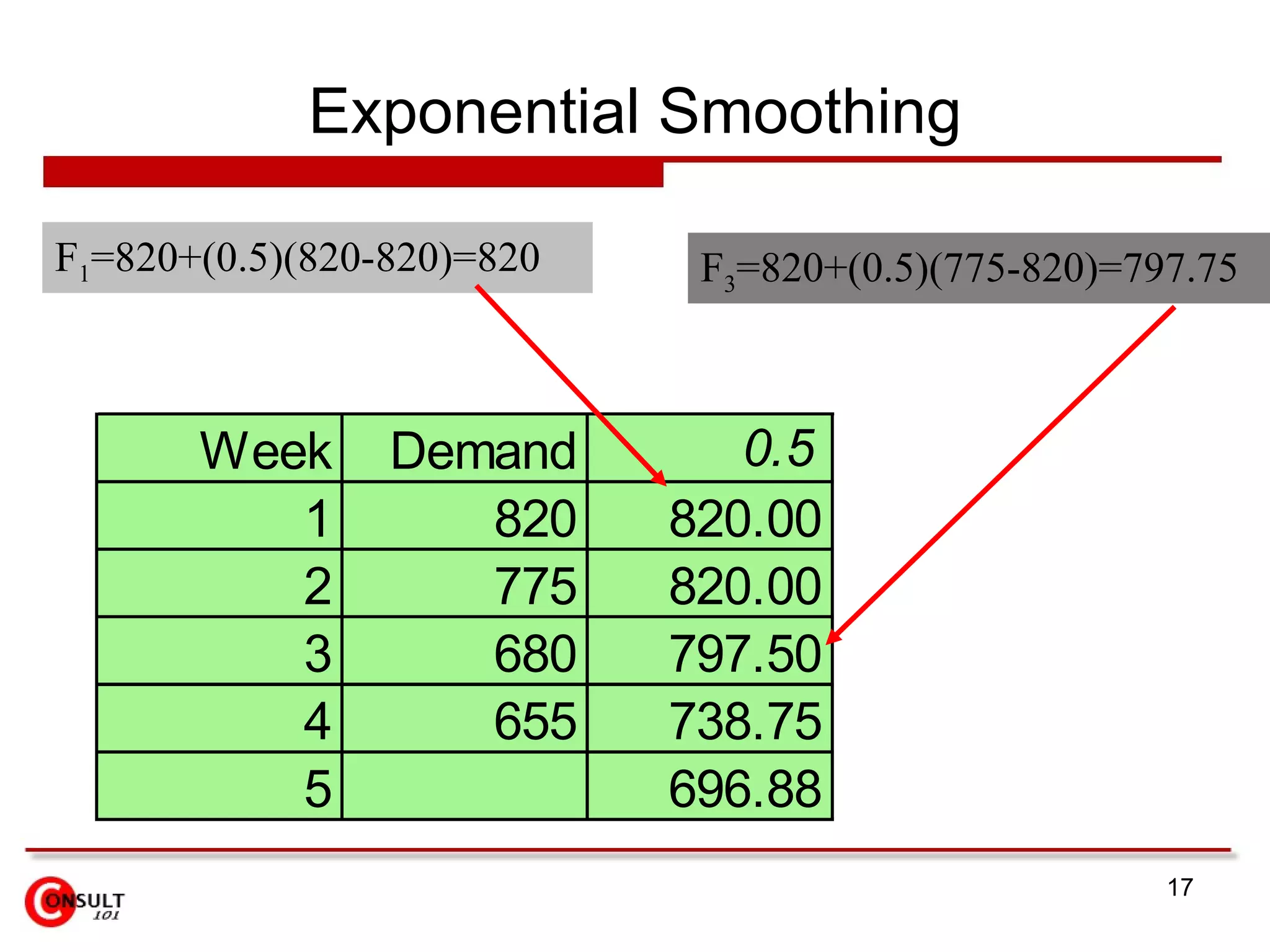
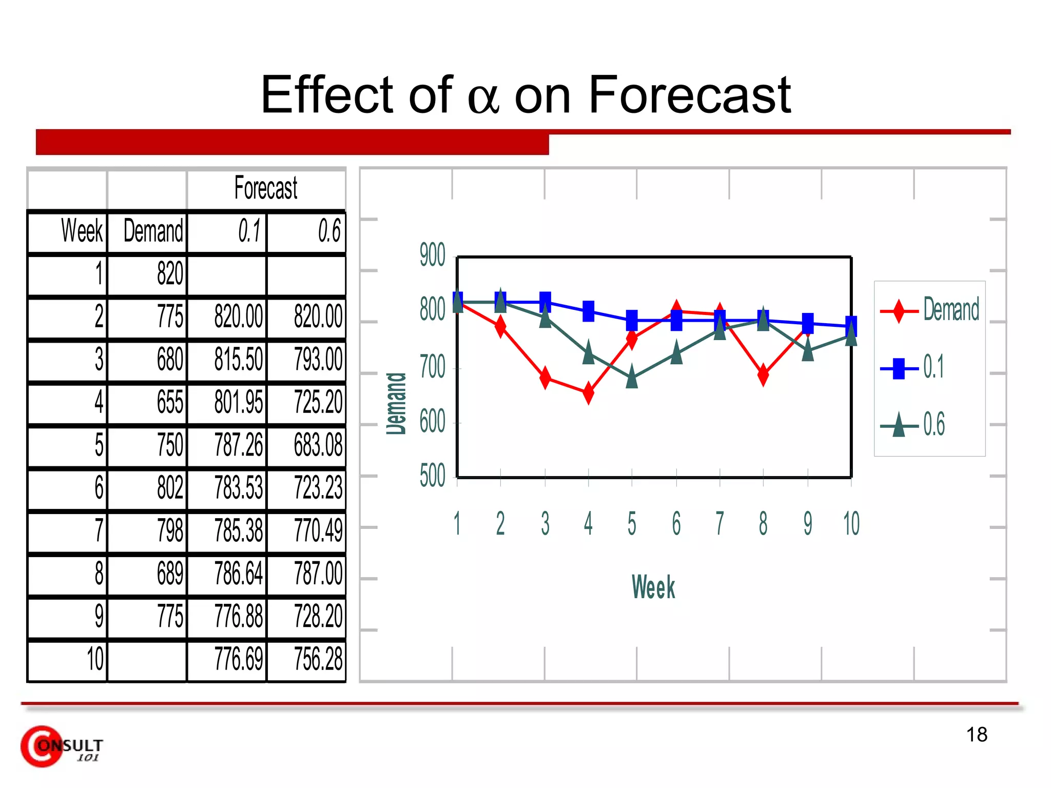
16. Exponential Smoothing Premise — determine how much weight to put on recent information versus older information 0 < a < 1 High a such as .7 puts weight on recent demand Low a such as .2 puts weight on many previous periods F t+1 =  D t + (1-  )F t (  is the smoothing parameter)

17. Exponential Smoothing F 1 =820+(0.5)(820-820)=820 F 3 =820+(0.5)(775-820)=797.75

18. Effect of  on Forecast

19. Simple Linear Regression Model

20. Simple Linear Regression Model (Contd)

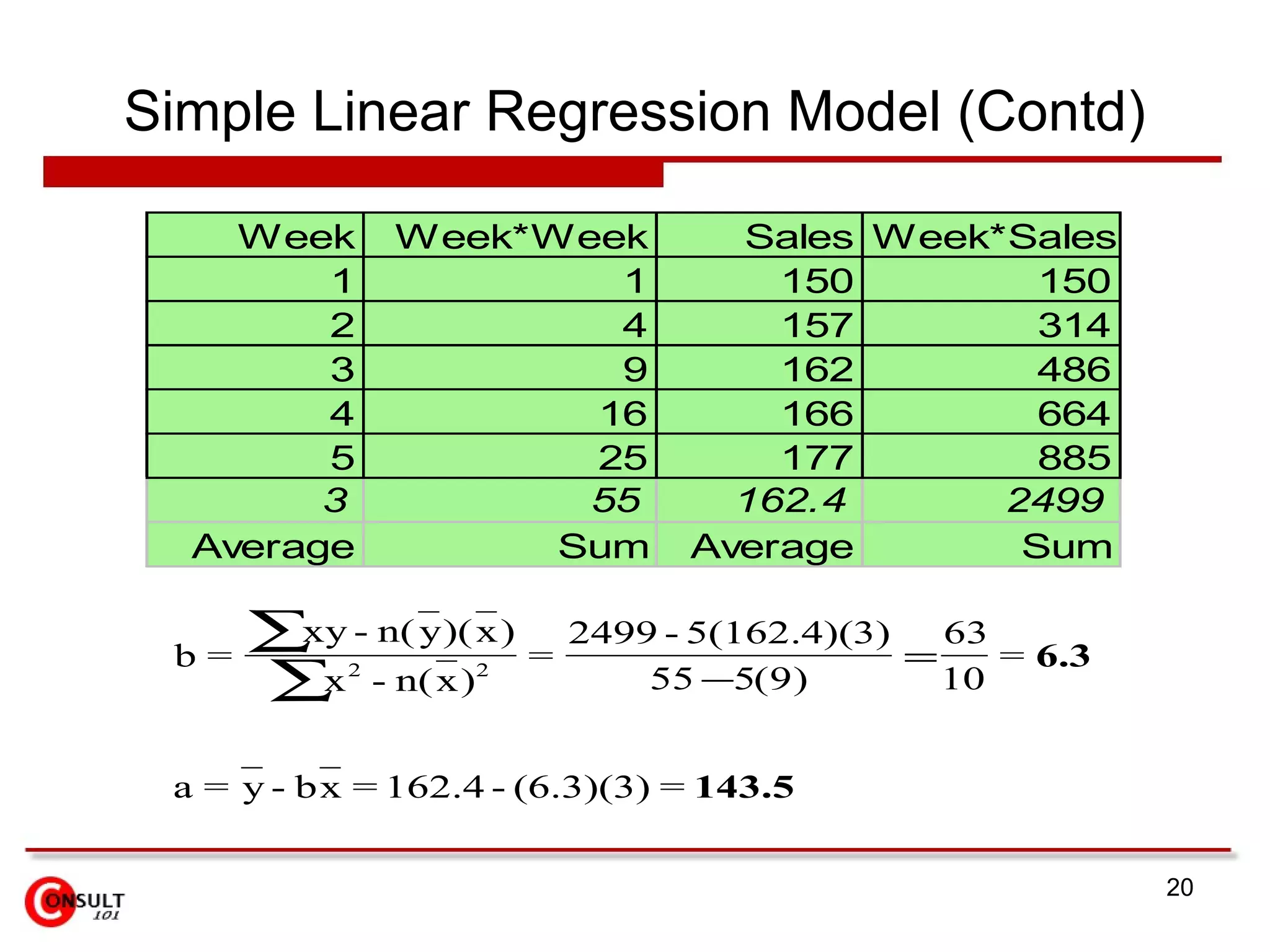
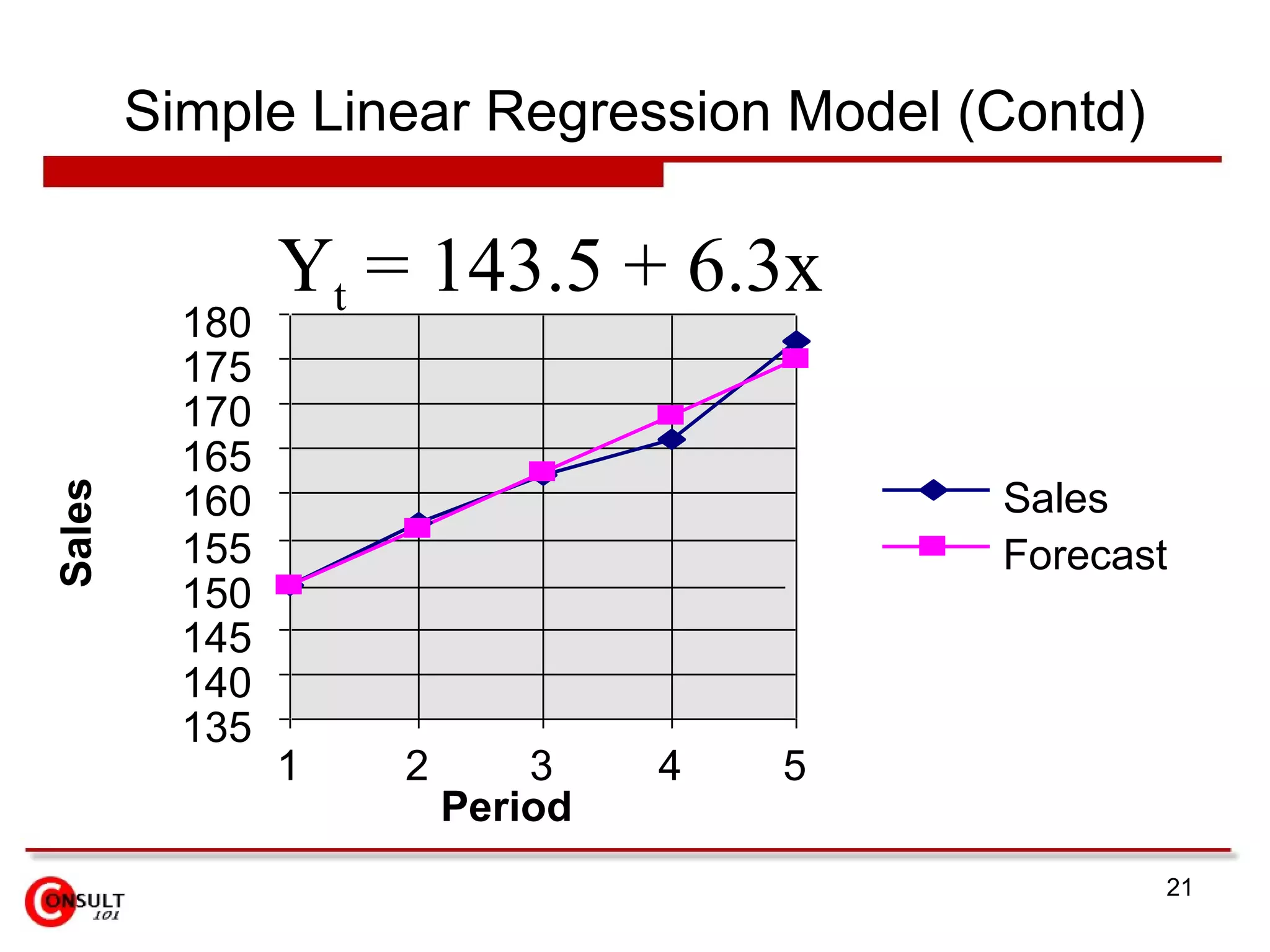
21. Simple Linear Regression Model (Contd) Y t = 143.5 + 6.3x 135 140 145 150 155 160 165 170 175 180 1 2 3 4 5 Period Sales Sales Forecast

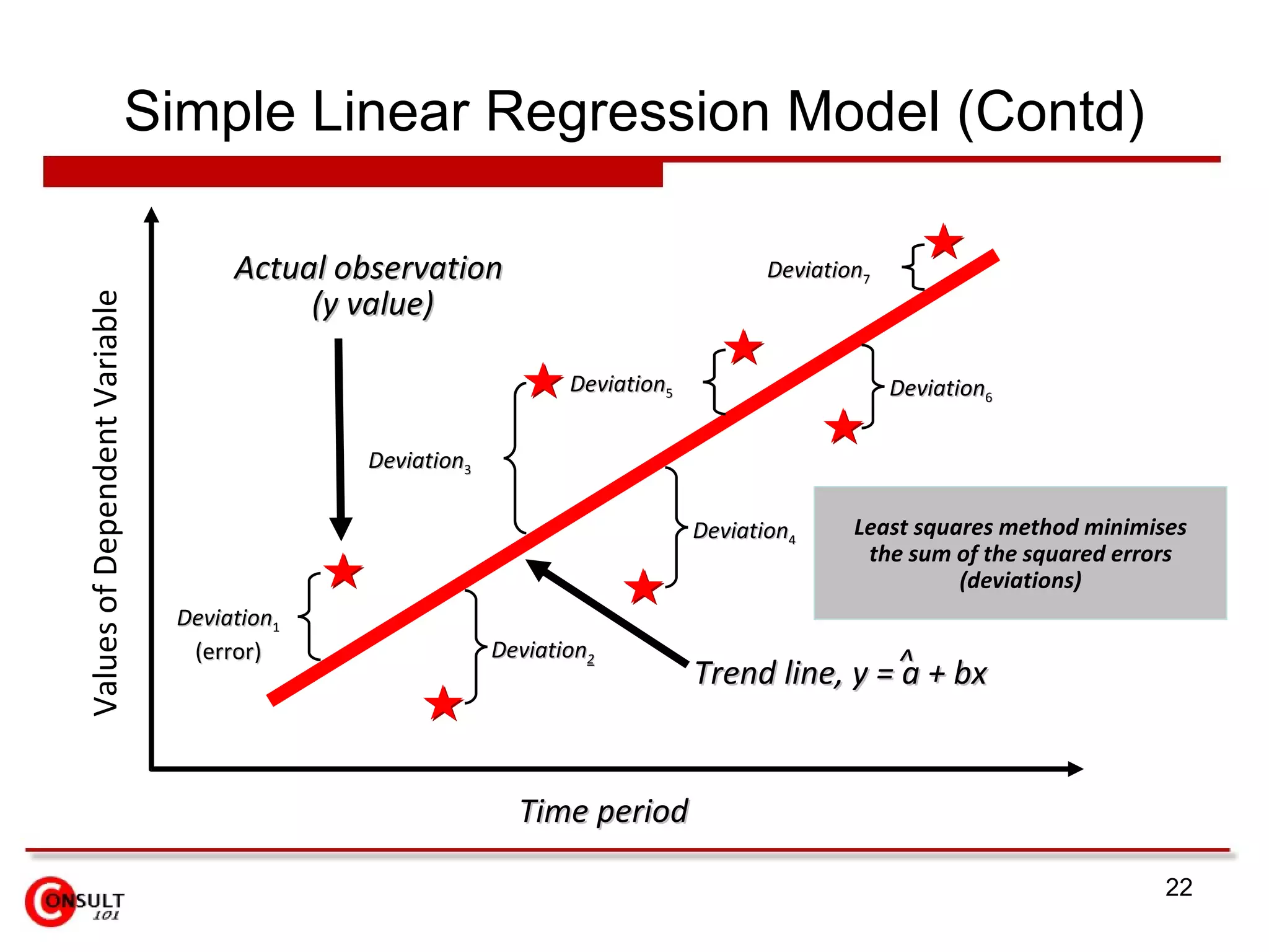
22. Simple Linear Regression Model (Contd) Actual observation (y value) Least squares method minimises the sum of the squared errors (deviations) Time period Values of Dependent Variable Deviation 1 (error) Deviation 5 Deviation 7 Deviation 2 Deviation 6 Deviation 4 Deviation 3 Trend line, y = a + bx ^

23. Forecast Accuracy / Error Reduction

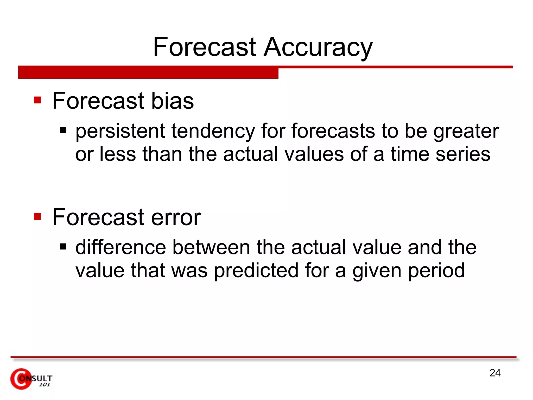
24. Forecast Accuracy Forecast bias persistent tendency for forecasts to be greater or less than the actual values of a time series Forecast error difference between the actual value and the value that was predicted for a given period

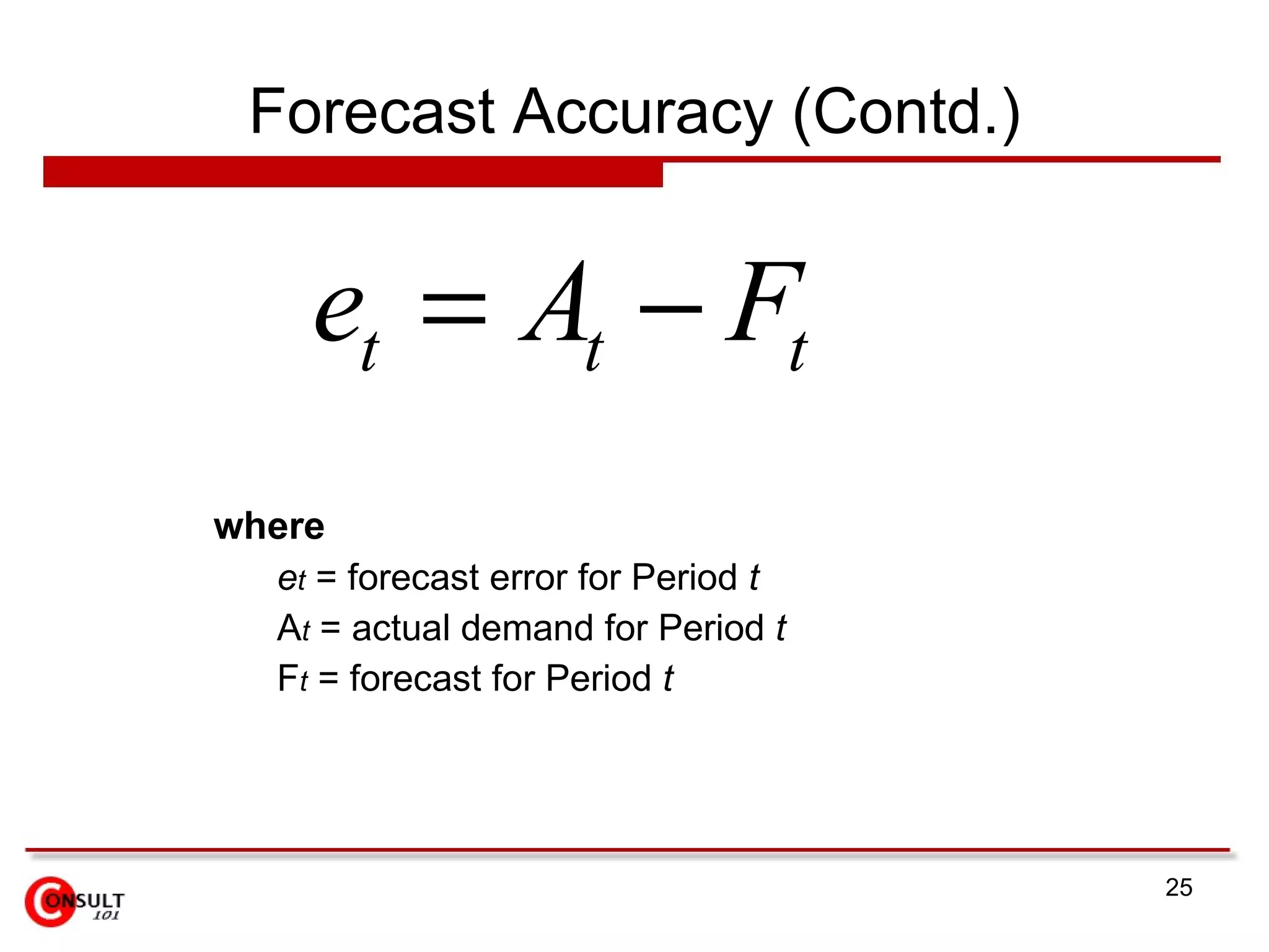
25. Forecast Accuracy (Contd.) where e t = forecast error for Period t A t = actual demand for Period t F t = forecast for Period t

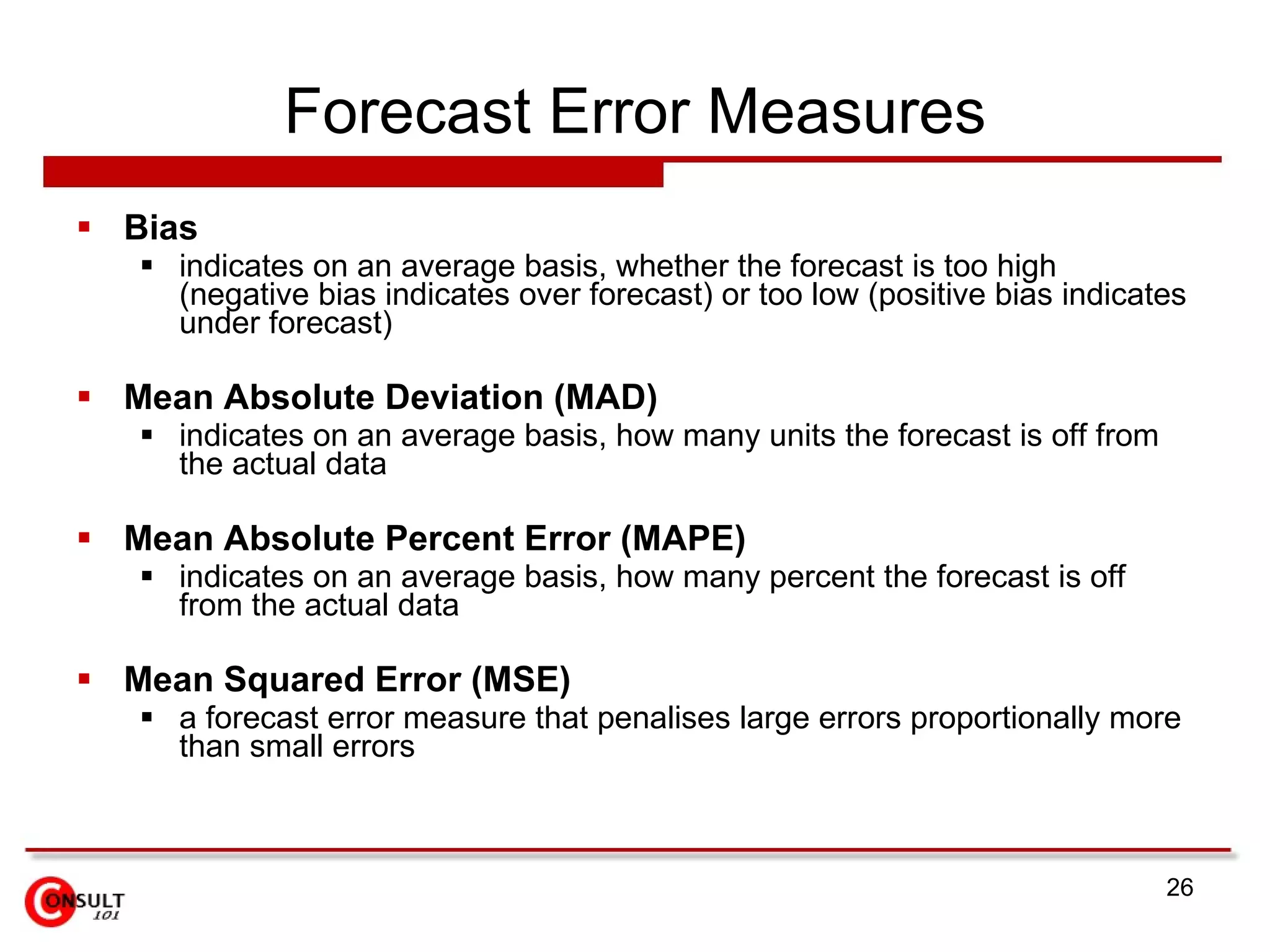
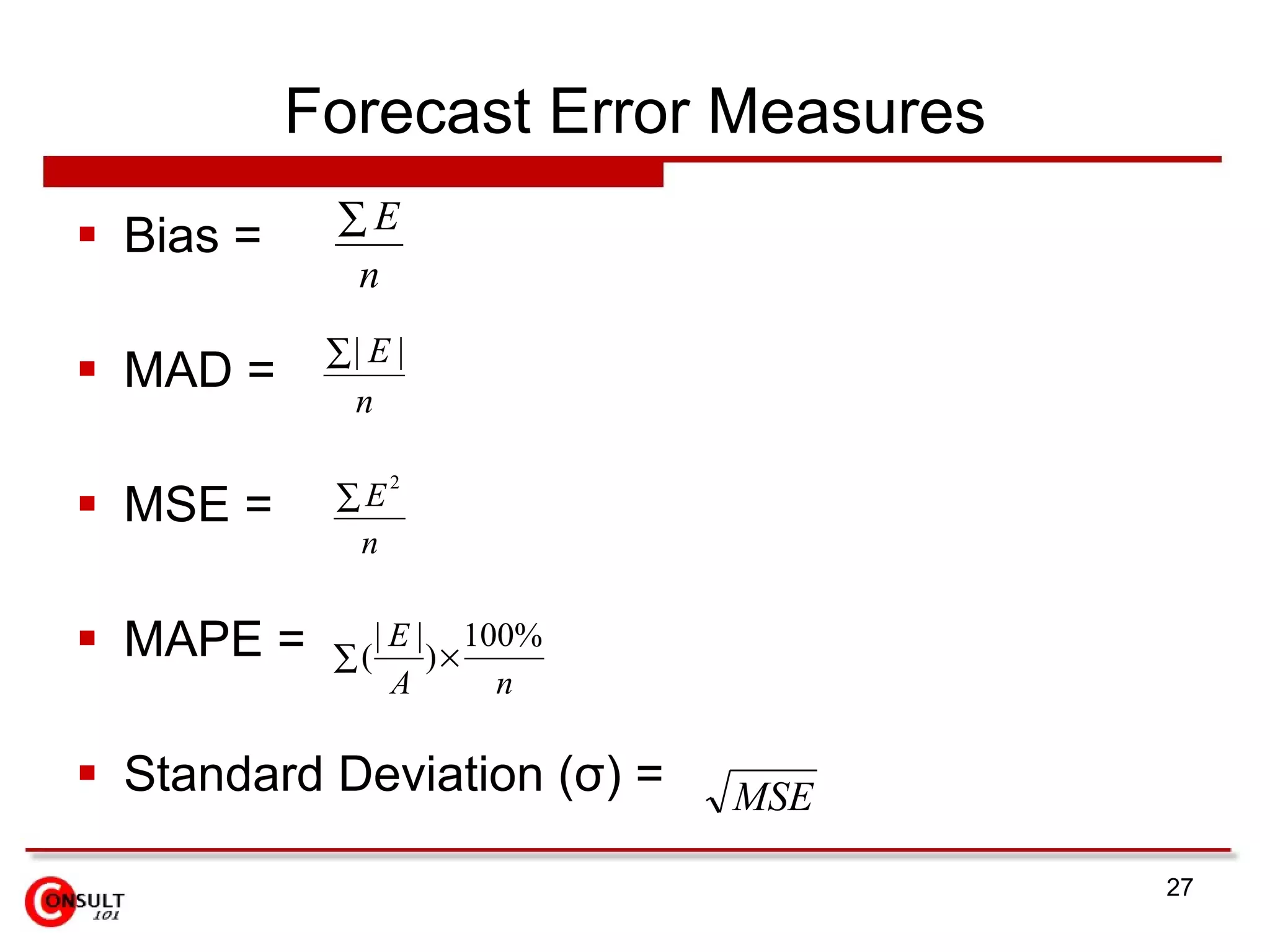
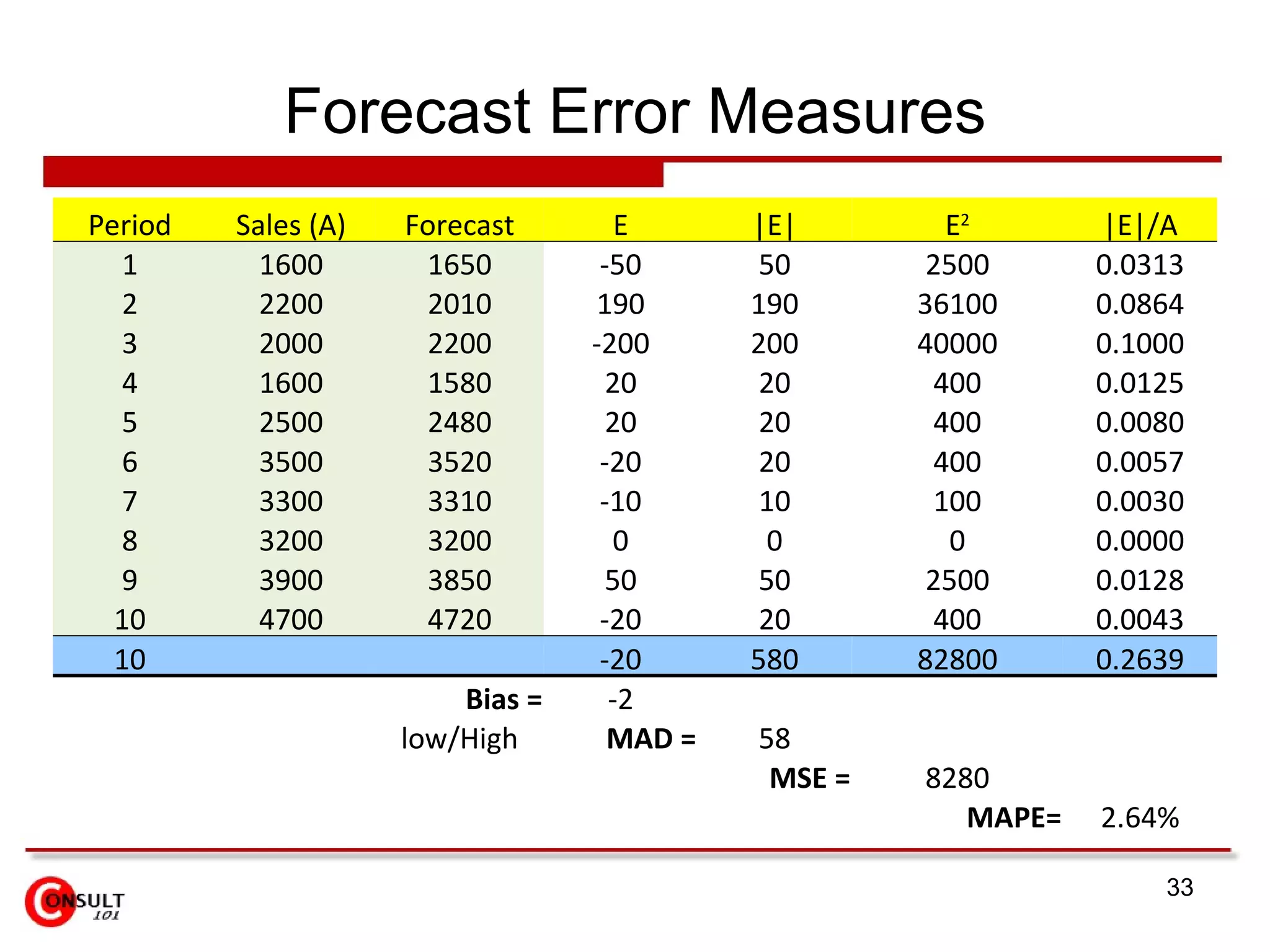
26. Forecast Error Measures Bias indicates on an average basis, whether the forecast is too high (negative bias indicates over forecast) or too low (positive bias indicates under forecast) Mean Absolute Deviation (MAD) indicates on an average basis, how many units the forecast is off from the actual data Mean Absolute Percent Error (MAPE) indicates on an average basis, how many percent the forecast is off from the actual data Mean Squared Error (MSE) a forecast error measure that penalises large errors proportionally more than small errors

27. Forecast Error Measures Bias = MAD = MSE = MAPE = Standard Deviation (σ) =

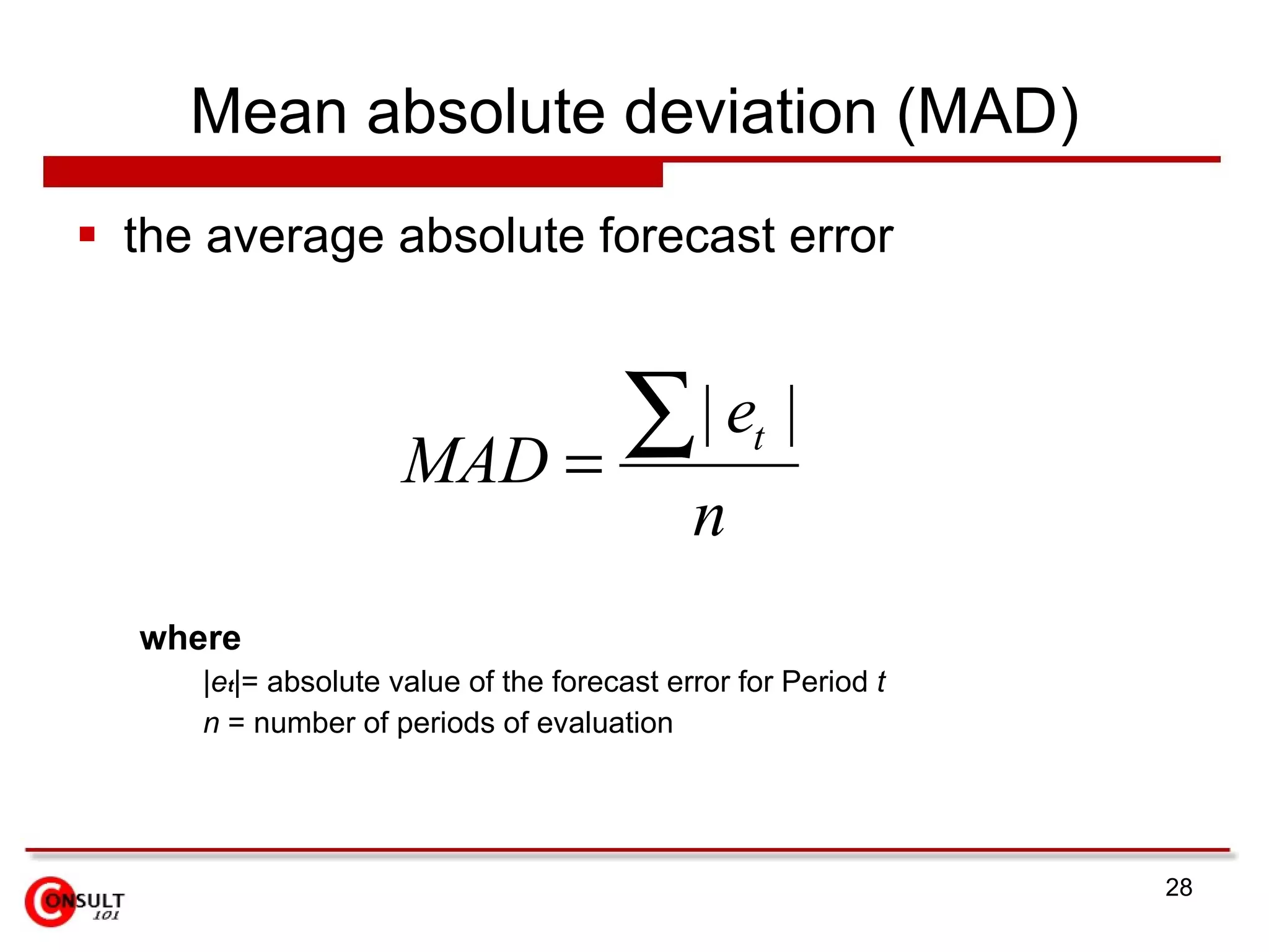
28. Mean absolute deviation (MAD) the average absolute forecast error where | e t |= absolute value of the forecast error for Period t n = number of periods of evaluation

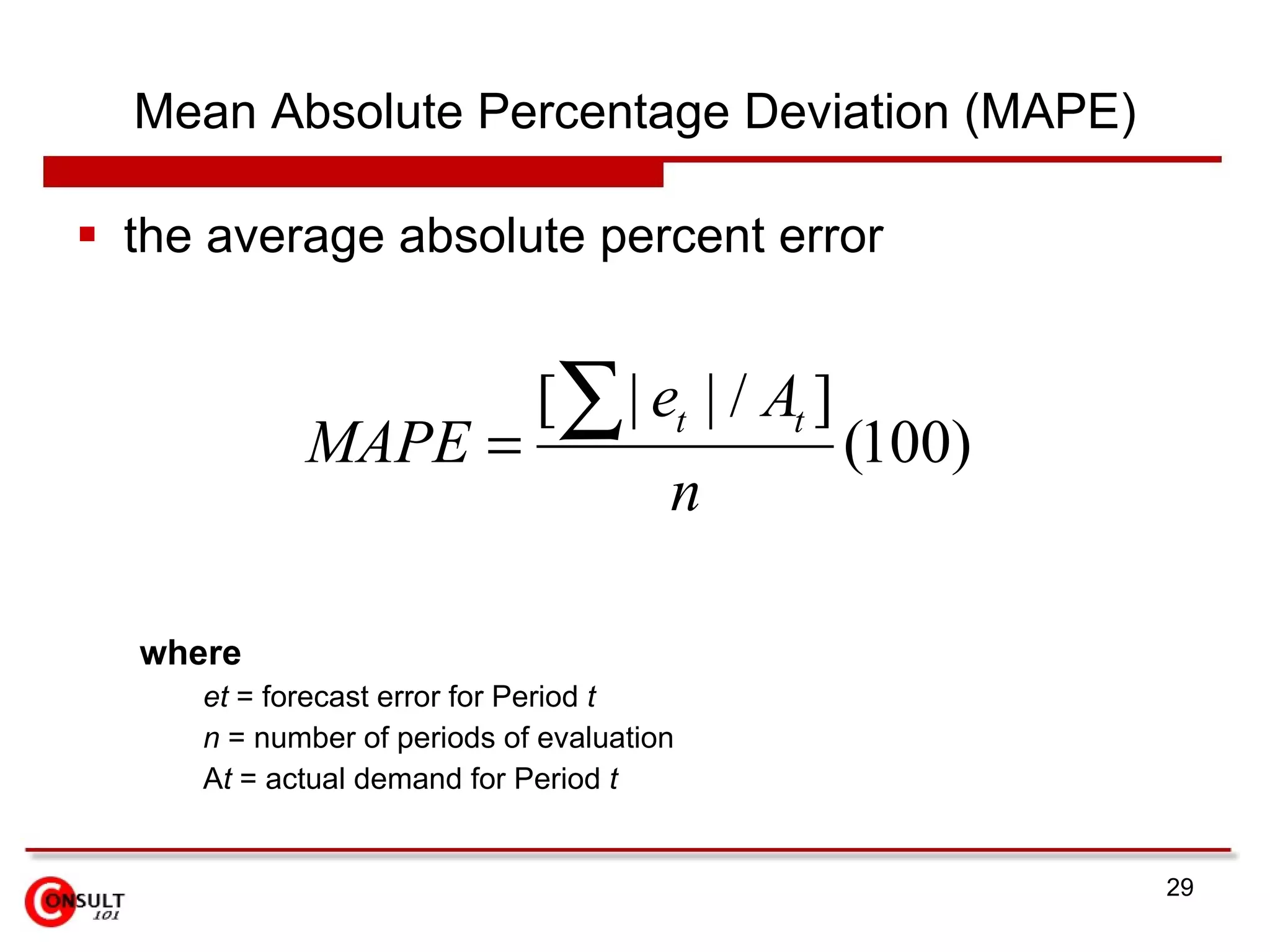
29. Mean Absolute Percentage Deviation (MAPE) the average absolute percent error where et = forecast error for Period t n = number of periods of evaluation A t = actual demand for Period t

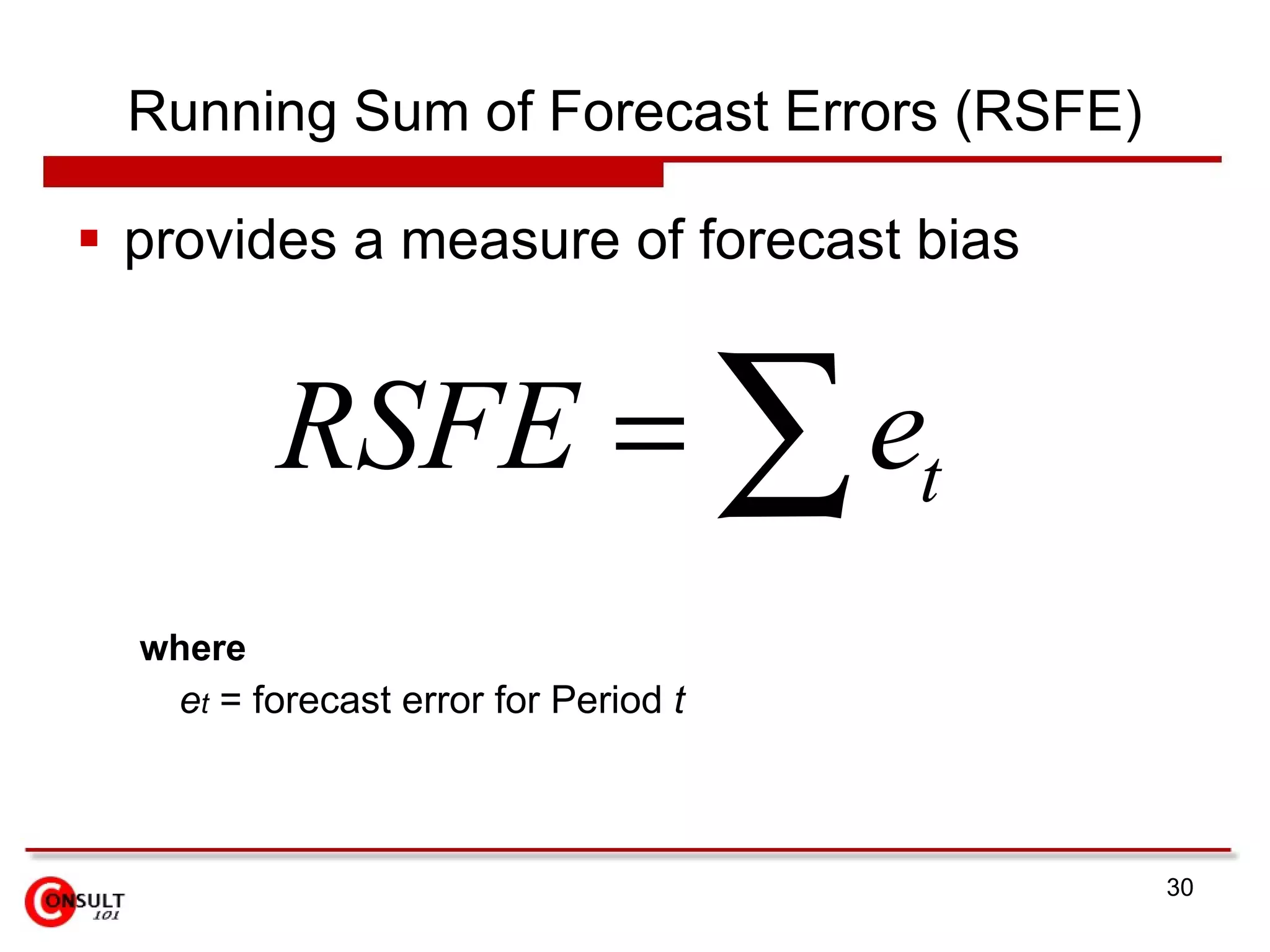
30. Running Sum of Forecast Errors (RSFE) provides a measure of forecast bias where e t = forecast error for Period t

31. Tracking Signal The ratio of cumulative forecast error to the corresponding value of MAD Used to monitor a forecast

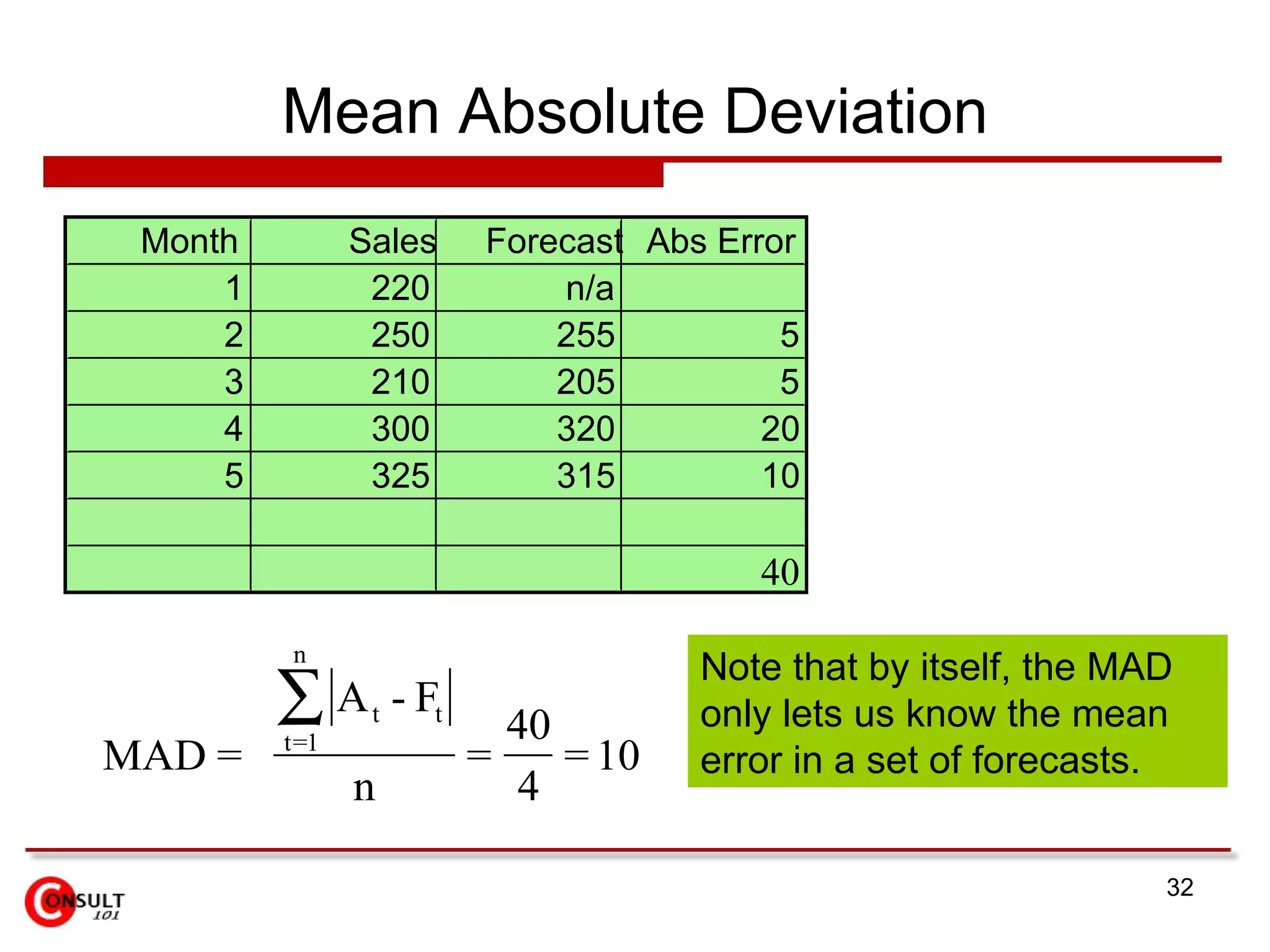
32. Mean Absolute Deviation Month Sales Forecast Abs Error 1 220 n/a 2 250 255 5 3 210 205 5 4 300 320 20 5 325 315 10 40 Note that by itself, the MAD only lets us know the mean error in a set of forecasts.

33. Forecast Error Measures Period Sales (A) Forecast E |E| E 2 |E|/A 1 1600 1650 -50 50 2500 0.0313 2 2200 2010 190 190 36100 0.0864 3 2000 2200 -200 200 40000 0.1000 4 1600 1580 20 20 400 0.0125 5 2500 2480 20 20 400 0.0080 6 3500 3520 -20 20 400 0.0057 7 3300 3310 -10 10 100 0.0030 8 3200 3200 0 0 0 0.0000 9 3900 3850 50 50 2500 0.0128 10 4700 4720 -20 20 400 0.0043 10 -20 580 82800 0.2639 Bias = -2 low/High MAD = 58 MSE = 8280 MAPE= 2.64%

34. Integrate – Sales Forecast / Production

35. Forecasting Process Services Collect Data Select Model Plot Data Develop Forecast Check Accuracy Forecast Adjust Forecast Monitor Forecast Sales and Operations Planning Master Scheduling Customer Scheduling Materials Planning Workforce Scheduling Order Scheduling Manufacturing Forecasting

36. Integrate - Sales Forecast & Production

37. CPFR - Collaborative Planning, Forecasting and Replenishment

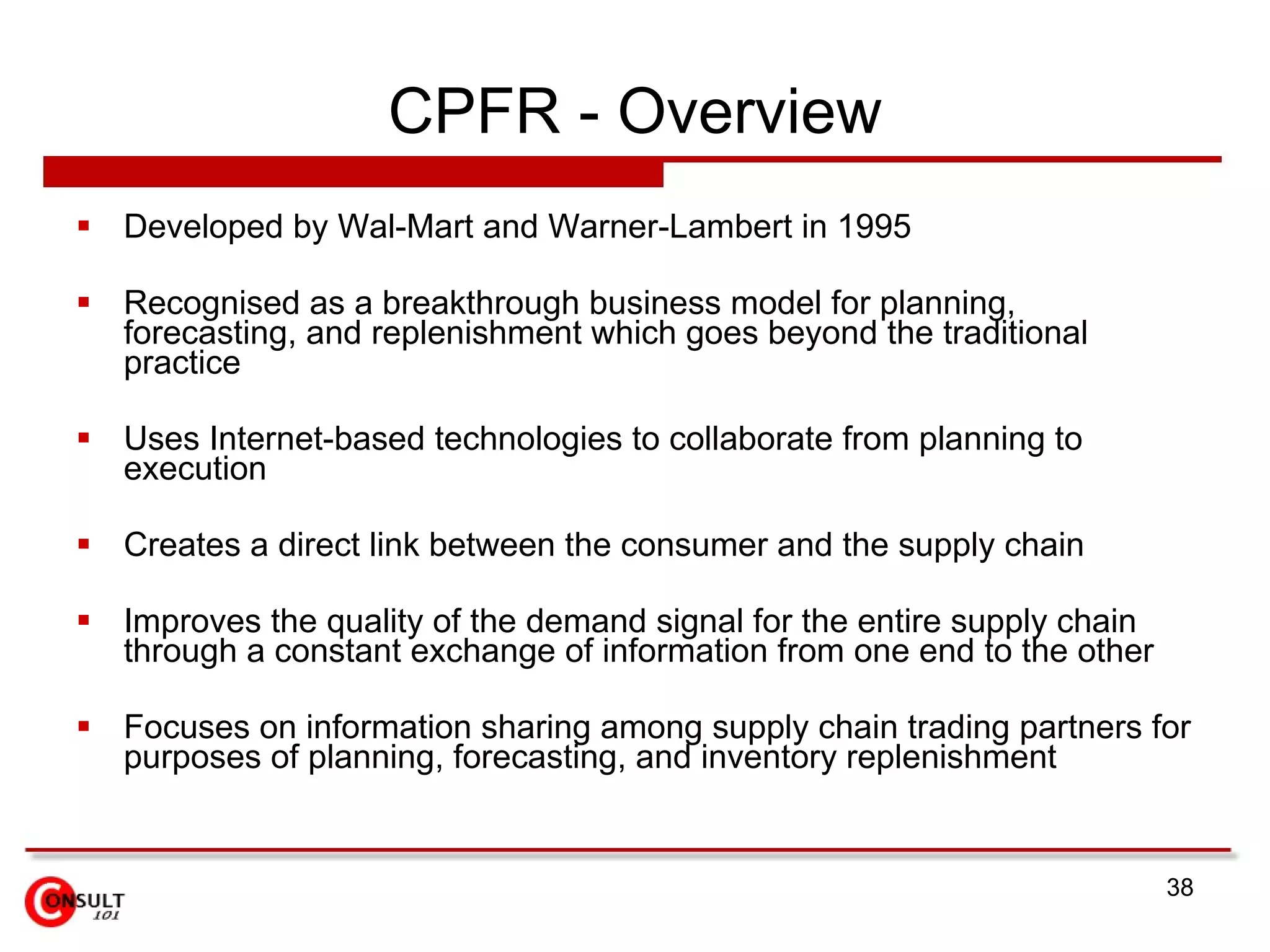
38. CPFR - Overview Developed by Wal-Mart and Warner-Lambert in 1995 Recognised as a breakthrough business model for planning, forecasting, and replenishment which goes beyond the traditional practice Uses Internet-based technologies to collaborate from planning to execution Creates a direct link between the consumer and the supply chain Improves the quality of the demand signal for the entire supply chain through a constant exchange of information from one end to the other Focuses on information sharing among supply chain trading partners for purposes of planning, forecasting, and inventory replenishment

39. CPFR Model

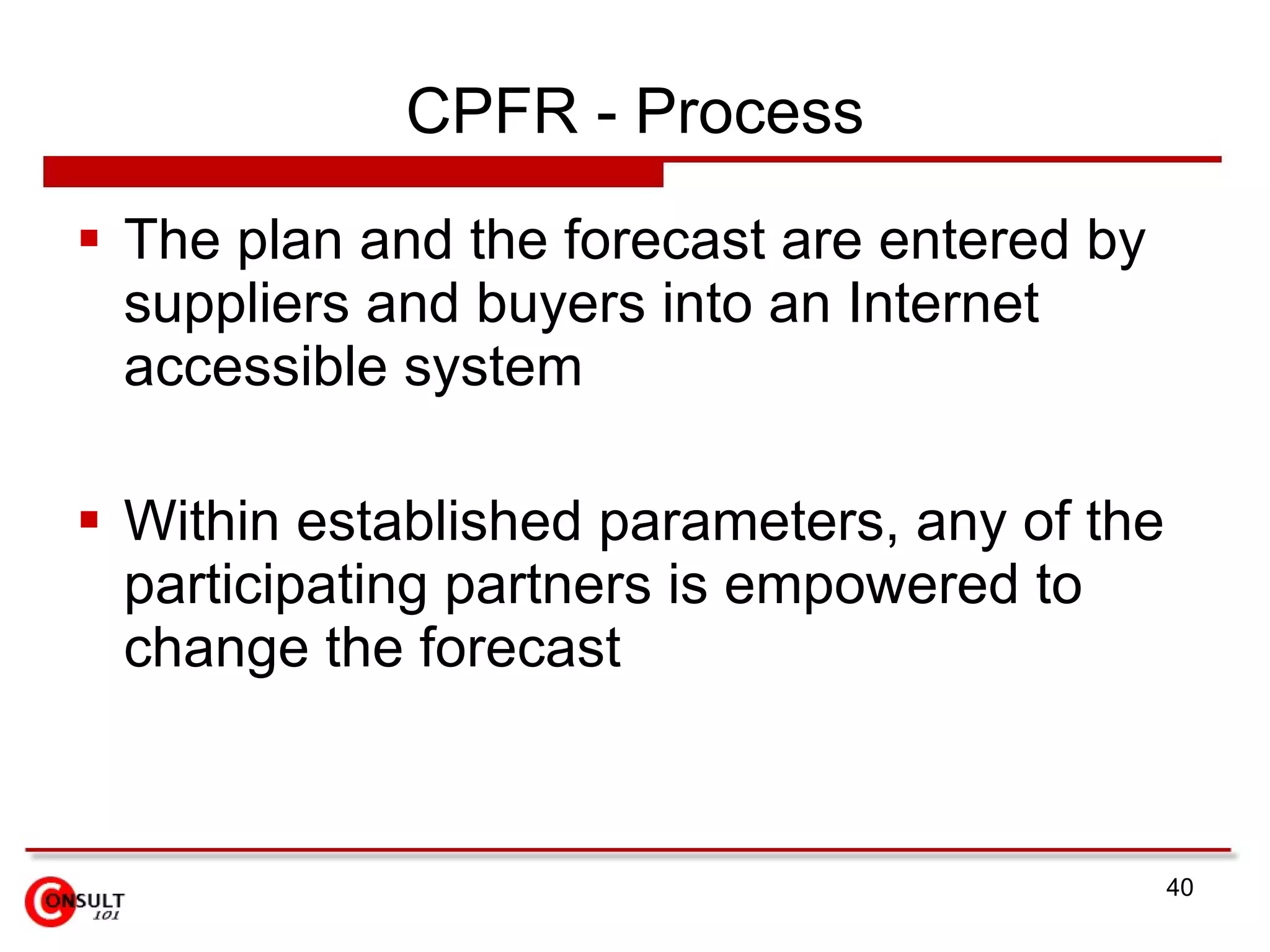
40. CPFR - Process The plan and the forecast are entered by suppliers and buyers into an Internet accessible system Within established parameters, any of the participating partners is empowered to change the forecast

41. “ You may have to fight a battle more than once to win it.” - Margaret Thatcher

42. Good Luck http://www.linkedin.com/in/anandsubramaniam