Here are the exponential smoothing forecasts for periods 2-10 using a smoothing constant (α) of 0.1:
2: 815.50
3: 801.95
4: 787.26
5: 783.53
6: 785.38
7: 786.64
8: 784.17
9: 782.29
10: 780.41
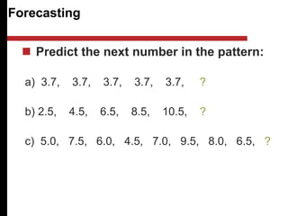
Forecasting
Predict thenext number in the pattern:
a) 3.7, 3.7, 3.7, 3.7, 3.7, ?
b) 2.5, 4.5, 6.5, 8.5, 10.5, ?
c) 5.0, 7.5, 6.0, 4.5, 7.0, 9.5, 8.0, 6.5, ?
3.
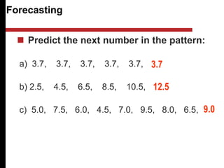
Forecasting
Predict thenext number in the pattern:
a) 3.7, 3.7, 3.7, 3.7, 3.7,
b) 2.5, 4.5, 6.5, 8.5, 10.5,
c) 5.0, 7.5, 6.0, 4.5, 7.0, 9.5, 8.0, 6.5,
3.7
12.5
9.0
4.
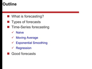
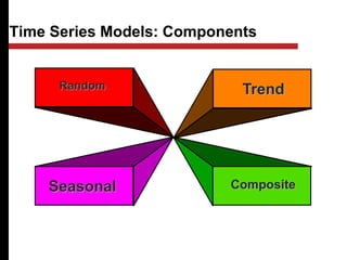
Outline
What isforecasting?
Types of forecasts
Time-Series forecasting
Naive
Moving Average
Exponential Smoothing
Regression
Good forecasts
5.
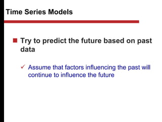
What is Forecasting?
Process of predicting a future
event based on historical data
Educated Guessing
Underlying basis of
all business decisions
Production
Inventory
Personnel
Facilities
6.
In general, forecastsare almost always wrong. So,
Why do we need to forecast?
Throughout the day we forecast very different
things such as weather, traffic, stock market, state
of our company from different perspectives.
Virtually every business attempt is based on
forecasting. Not all of them are derived from
sophisticated methods. However, “Best" educated
guesses about future are more valuable for
purpose of Planning than no forecasts and hence
no planning.
7.
Departments throughout theorganization depend on
forecasts to formulate and execute their plans.
Finance needs forecasts to project cash flows and
capital requirements.
Human resources need forecasts to anticipate hiring
needs.
Production needs forecasts to plan production
levels, workforce, material requirements,
inventories, etc.
Importance of Forecasting in PPC
8.
Demand is notthe only variable of interest to
forecasters.
Manufacturers also forecast worker absenteeism,
machine availability, material costs, transportation
and production lead times, etc.
Besides demand, service providers are also
interested in forecasts of population, of other
demographic variables, of weather, etc.
Importance of Forecasting in PPC
9.
Definition of forecasting
In literary sense forecasting means
prediction. It may be defined as a technique
of translating past experience into
prediction of things to come.
10.
OBJECTIVES OF FORECASTING
Short term objectives
• Formulation of suitable production policy.
• Regulate supply of raw material.
• Best utilization of machines.
• Regular availability of labor.
• Price policy formulation.
• Forecasting of short term financial
requirements.
• Setting the sales target.
11.
Long term objectives
•Deciding plant capacity.
• Manpower planning.
• Estimating cash inflows.
• Determining dividend policy.
• Planning of long-run production.
• Long run of financial requirements.
• Budgetary control over expenditure.
12.
Factors affecting forecasting
•General business conditions.
• Conditions within the industry.
• Conditions within the company.
• Factors affecting export trade.
• Political stability.
• Government restrictions.
• Fiscal and monetary policy.
• Price level and trend.
• Technological research and development.
13.
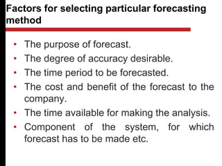
Factors for selectingparticular forecasting
method
• The purpose of forecast.
• The degree of accuracy desirable.
• The time period to be forecasted.
• The cost and benefit of the forecast to the
company.
• The time available for making the analysis.
• Component of the system, for which
forecast has to be made etc.
14.
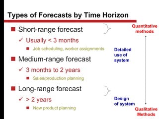
Short-range forecast
Usually < 3 months
Job scheduling, worker assignments
Medium-range forecast
3 months to 2 years
Sales/production planning
Long-range forecast
> 2 years
New product planning
Types of Forecasts by Time Horizon
Design
of system
Detailed
use of
system
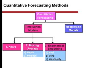
Quantitative
methods
Qualitative
Methods
15.
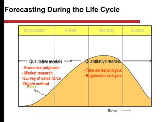
Forecasting During theLife Cycle
Introduction Growth Maturity Decline
Sales
Time
Quantitative models
- Time series analysis
- Regression analysis
Qualitative models
- Executive judgment
- Market research
-Survey of sales force
-Delphi method
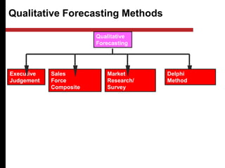
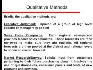
Briefly, the qualitativemethods are:
Executive Judgment: Opinion of a group of high level
experts or managers is pooled
Sales Force Composite: Each regional salesperson
provides his/her sales estimates. Those forecasts are then
reviewed to make sure they are realistic. All regional
forecasts are then pooled at the district and national levels
to obtain an overall forecast.
Market Research/Survey: Solicits input from customers
pertaining to their future purchasing plans. It involves the
use of questionnaires, consumer panels and tests of new
products and services.
Qualitative Methods
18.
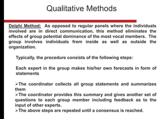
Delphi Method: Asopposed to regular panels where the individuals
involved are in direct communication, this method eliminates the
effects of group potential dominance of the most vocal members. The
group involves individuals from inside as well as outside the
organization.
Typically, the procedure consists of the following steps:
Each expert in the group makes his/her own forecasts in form of
statements
The coordinator collects all group statements and summarizes
them
The coordinator provides this summary and gives another set of
questions to each group member including feedback as to the
input of other experts.
The above steps are repeated until a consensus is reached.
Qualitative Methods
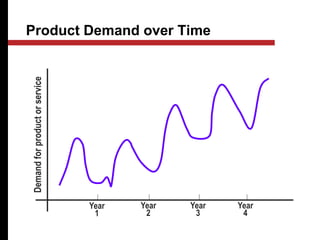
Product Demand overTime
Year
1
Year
2
Year
3
Year
4
Demand
for
product
or
service
24.
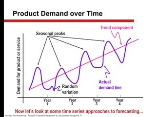
Product Demand overTime
Year
1
Year
2
Year
3
Year
4
Demand
for
product
or
service
Trend component
Actual
demand line
Seasonal peaks
Random
variation
Now let’s look at some time series approaches to forecasting…
Borrowed from Heizer/Render - Principles of Operations Management, 5e, and Operations Management, 7e
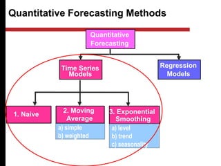
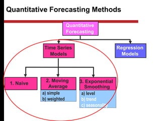
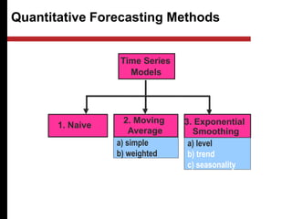
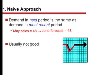
1. Naive Approach
Demand in next period is the same as
demand in most recent period
May sales = 48 →
Usually not good
June forecast = 48
27.
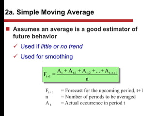
2a. Simple MovingAverage
n
A
+
...
+
A
+
A
+
A
=
F 1
n
-
t
2
-
t
1
-
t
t
1
t
Assumes an average is a good estimator of
future behavior
Used if little or no trend
Used for smoothing
Ft+1 = Forecast for the upcoming period, t+1
n = Number of periods to be averaged
A t = Actual occurrence in period t
28.
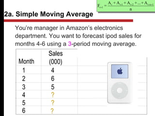
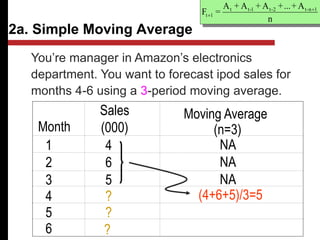
2a. Simple MovingAverage
You’re manager in Amazon’s electronics
department. You want to forecast ipod sales for
months 4-6 using a 3-period moving average.
n
A
+
...
+
A
+
A
+
A
=
F 1
n
-
t
2
-
t
1
-
t
t
1
t
Month
Sales
(000)
1 4
2 6
3 5
4 ?
5 ?
6 ?
29.
2a. Simple MovingAverage
Month
Sales
(000)
Moving Average
(n=3)
1 4 NA
2 6 NA
3 5 NA
4 ?
5 ?
(4+6+5)/3=5
6 ?
n
A
+
...
+
A
+
A
+
A
=
F 1
n
-
t
2
-
t
1
-
t
t
1
t
You’re manager in Amazon’s electronics
department. You want to forecast ipod sales for
months 4-6 using a 3-period moving average.
30.
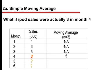
What if ipodsales were actually 3 in month 4
Month
Sales
(000)
Moving Average
(n=3)
1 4 NA
2 6 NA
3 5 NA
4 3
5 ?
5
6 ?
2a. Simple Moving Average
?
31.
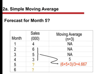
Forecast for Month5?
Month
Sales
(000)
Moving Average
(n=3)
1 4 NA
2 6 NA
3 5 NA
4 3
5 ?
5
6 ?
(6+5+3)/3=4.667
2a. Simple Moving Average
32.
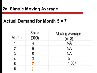
Actual Demand forMonth 5 = 7
Month
Sales
(000)
Moving Average
(n=3)
1 4 NA
2 6 NA
3 5 NA
4 3
5 7
5
6 ?
4.667
2a. Simple Moving Average
?
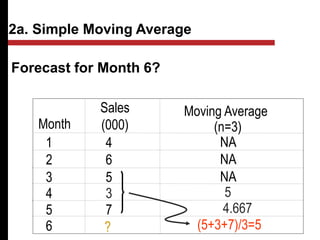
33.
Forecast for Month6?
Month
Sales
(000)
Moving Average
(n=3)
1 4 NA
2 6 NA
3 5 NA
4 3
5 7
5
6 ?
4.667
(5+3+7)/3=5
2a. Simple Moving Average
34.
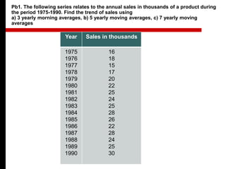
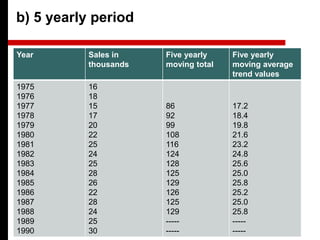
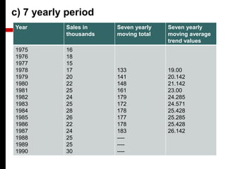
Pb1. The followingseries relates to the annual sales in thousands of a product during
the period 1975-1990. Find the trend of sales using
a) 3 yearly morning averages, b) 5 yearly moving averages, c) 7 yearly moving
averages
Year Sales in thousands
1975
1976
1977
1978
1979
1980
1981
1982
1983
1984
1985
1986
1987
1988
1989
1990
16
18
15
17
20
22
25
24
25
28
26
22
28
24
25
30
35.
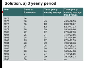
Solution. a) 3yearly period
Year Sales in
thousands
Three yearly
moving average
Three yearly
moving average
trend values
1975
1976
1977
1978
1979
1980
1981
1982
1983
1984
1985
1986
1987
1988
1989
1990
16
18
15
17
20
22
25
24
25
28
26
22
28
24
25
30
49
50
52
59
67
71
74
67
79
76
76
74
77
79
---
49/3=16.33
50/3=16.67
52/3=17.33
59/3=19.66
67/3=22.33
71/3=23.66
74/3=24.66
67/3=22.33
79/3=26.33
76/3=25.33
76/3=25.33
74/3=24.66
77/3=25.66
79/3=26.33
----
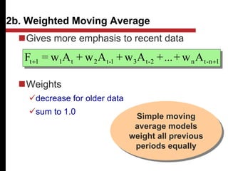
Gives more emphasisto recent data
Weights
decrease for older data
sum to 1.0
2b. Weighted Moving Average
1
n
-
t
n
2
-
t
3
1
-
t
2
t
1
1
t A
w
+
...
+
A
w
+
A
w
+
A
w
=
F
Simple moving
average models
weight all previous
periods equally
39.
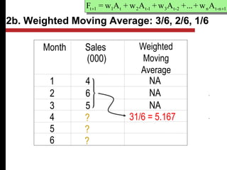
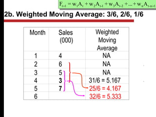
2b. Weighted MovingAverage: 3/6, 2/6, 1/6
Month Weighted
Moving
Average
1 4 NA
2 6 NA
3 5 NA
4 31/6 = 5.167
5
6 ?
?
?
1
n
-
t
n
2
-
t
3
1
-
t
2
t
1
1
t A
w
+
...
+
A
w
+
A
w
+
A
w
=
F
Sales
(000)
40.
2b. Weighted MovingAverage: 3/6, 2/6, 1/6
Month Sales
(000)
Weighted
Moving
Average
1 4 NA
2 6 NA
3 5 NA
4 3 31/6 = 5.167
5 7
6
25/6 = 4.167
32/6 = 5.333
1
n
-
t
n
2
-
t
3
1
-
t
2
t
1
1
t A
w
+
...
+
A
w
+
A
w
+
A
w
=
F
41.
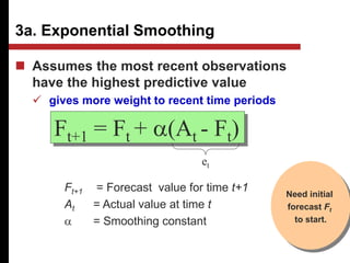
3a. Exponential Smoothing
Assumes the most recent observations
have the highest predictive value
gives more weight to recent time periods
Ft+1 = Ft + a(At - Ft)
et
Ft+1 = Forecast value for time t+1
At = Actual value at time t
a = Smoothing constant
Need initial
forecast Ft
to start.
42.
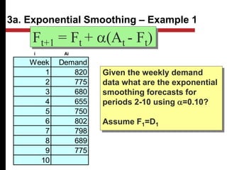
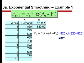
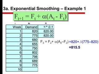
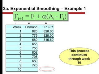
3a. Exponential Smoothing– Example 1
Week Demand
1 820
2 775
3 680
4 655
5 750
6 802
7 798
8 689
9 775
10
Given the weekly demand
data what are the exponential
smoothing forecasts for
periods 2-10 using a=0.10?
Assume F1=D1
Ft+1 = Ft + a(At - Ft)
i Ai
Week Demand 0.10.6
1 820 820.00 820.00
2 775 820.00 820.00
3 680 815.50 793.00
4 655 801.95 725.20
5 750 787.26 683.08
6 802 783.53 723.23
7 798 785.38 770.49
8 689 786.64 787.00
9 775 776.88 728.20
10 776.69 756.28
Ft+1 = Ft + a(At - Ft)
This process
continues
through week
10
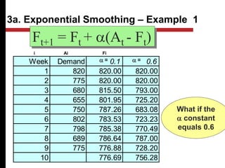
3a. Exponential Smoothing – Example 1
a =
i Ai Fi
46.
Week Demand 0.10.6
1 820 820.00 820.00
2 775 820.00 820.00
3 680 815.50 793.00
4 655 801.95 725.20
5 750 787.26 683.08
6 802 783.53 723.23
7 798 785.38 770.49
8 689 786.64 787.00
9 775 776.88 728.20
10 776.69 756.28
Ft+1 = Ft + a(At - Ft)
What if the
a constant
equals 0.6
3a. Exponential Smoothing – Example 1
a = a =
i Ai Fi
47.
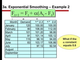
Month Demand 0.30.6
January 120 100.00 100.00
February 90 106.00 112.00
March 101 101.20 98.80
April 91 101.14 100.12
May 115 98.10 94.65
June 83 103.17 106.86
July 97.12 92.54
August
September
Ft+1 = Ft + a(At - Ft)
What if the
a constant
equals 0.6
3a. Exponential Smoothing – Example 2
a = a =
i Ai Fi
48.
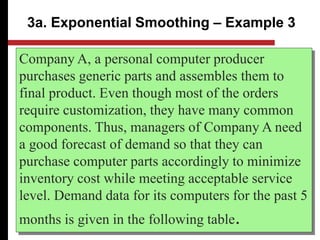
Company A, apersonal computer producer
purchases generic parts and assembles them to
final product. Even though most of the orders
require customization, they have many common
components. Thus, managers of Company A need
a good forecast of demand so that they can
purchase computer parts accordingly to minimize
inventory cost while meeting acceptable service
level. Demand data for its computers for the past 5
months is given in the following table.
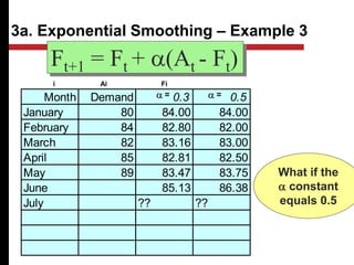
3a. Exponential Smoothing – Example 3
49.
Month Demand 0.30.5
January 80 84.00 84.00
February 84 82.80 82.00
March 82 83.16 83.00
April 85 82.81 82.50
May 89 83.47 83.75
June 85.13 86.38
July ?? ??
Ft+1 = Ft + a(At - Ft)
What if the
a constant
equals 0.5
3a. Exponential Smoothing – Example 3
a = a =
i Ai Fi
50.
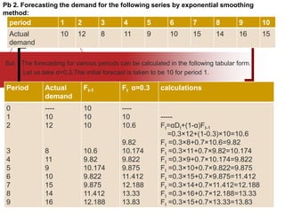
Sol. The forecastingfor various periods can be calculated in the following tabular form.
Let us take α=0.3.The initial forecast is taken to be 10 for period 1.
Pb 2. Forecasting the demand for the following series by exponential smoothing
method:
period 1 2 3 4 5 6 7 8 9 10
Actual
demand
10 12 8 11 9 10 15 14 16 15
Period Actual
demand
Ft-1 Ft α=0.3 calculations
0
1
2
3
4
5
6
7
8
9
----
10
12
8
11
9
10
15
14
16
10
10
10
10.6
9.82
10.174
9.822
9.875
11.412
12.188
----
10
10.6
9.82
10.174
9.822
9.875
11.412
12.188
13.33
13.83
-----
Ft=αDt+(1-α)Ft-1
=0.3×12+(1-0.3)×10=10.6
Ft =0.3×8+0.7×10.6=9.82
Ft =0.3×11+0.7×9.82=10.174
Ft =0.3×9+0.7×10.174=9.822
Ft =0.3×10+0.7×9.822=9.875
Ft =0.3×15+0.7×9.875=11.412
Ft =0.3×14+0.7×11.412=12.188
Ft =0.3×16+0.7×12.188=13.33
Ft =0.3×15+0.7×13.33=13.83
51.
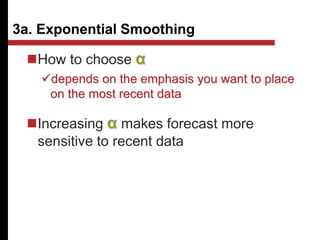
How to chooseα
depends on the emphasis you want to place
on the most recent data
Increasing α makes forecast more
sensitive to recent data
3a. Exponential Smoothing
52.
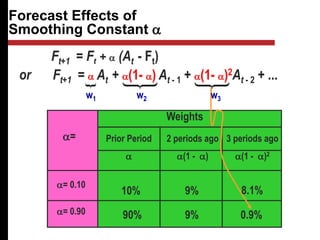
Ft+1 = aAt + a(1- a) At - 1 + a(1- a)2At - 2 + ...
Forecast Effects of
Smoothing Constant a
Weights
Prior Period
a
2 periods ago
a(1 - a)
3 periods ago
a(1 - a)2
a=
a= 0.10
a= 0.90
10% 9% 8.1%
90% 9% 0.9%
Ft+1 = Ft + a (At - Ft)
or
w1 w2 w3
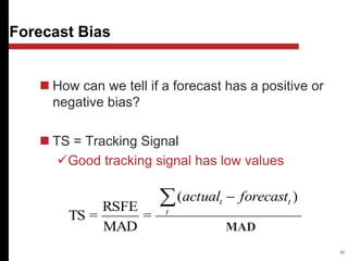
53.
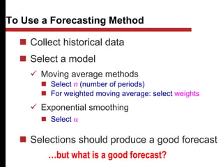
Collect historicaldata
Select a model
Moving average methods
Select n (number of periods)
For weighted moving average: select weights
Exponential smoothing
Select a
Selections should produce a good forecast
To Use a Forecasting Method
…but what is a good forecast?
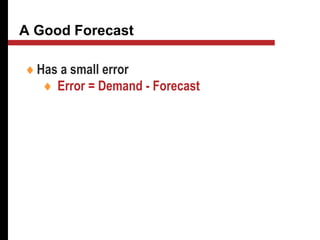
Measures of ForecastError
b. MSE = Mean Squared Error
n
F
-
A
=
MSE
n
1
=
t
2
t
t
MAD =
A - F
n
t t
t=1
n
et
Ideal values =0 (i.e., no forecasting error)
MSE
=
RMSE
c. RMSE = Root Mean Squared Error
a. MAD = Mean Absolute Deviation
56.
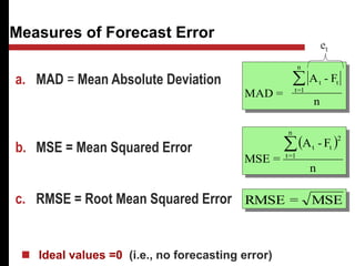
MAD Example
Month SalesForecast
1 220 n/a
2 250 255
3 210 205
4 300 320
5 325 315
What is the MAD value given the
forecast values in the table below?
MAD =
A - F
n
t t
t=1
n
5
5
20
10
|At – Ft|
Ft
At
= 40
= 40
4
=10
57.
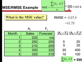
MSE/RMSE Example
Month SalesForecast
1 220 n/a
2 250 255
3 210 205
4 300 320
5 325 315
What is the MSE value?
5
5
20
10
|At – Ft|
Ft
At
= 550
4
=137.5
(At – Ft)2
25
25
400
100
= 550
n
F
-
A
=
MSE
n
1
=
t
2
t
t
RMSE = √137.5
=11.73
58.
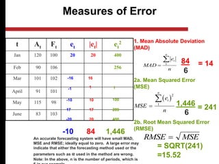
Measures of Error
tAt Ft et |et| et
2
Jan 120 100 20 20 400
Feb 90 106 256
Mar 101 102
April 91 101
May 115 98
June 83 103
1. Mean Absolute Deviation
(MAD)
n
e
MAD
n
t
1
2a. Mean Squared Error
(MSE)
MSE
e
n
t
n
2
1
2b. Root Mean Squared Error
(RMSE)
RMSE MSE
-16 16
-1 1
-10
17
-20
10
17
20
1
100
289
400
-10 84 1,446
84
6
= 14
1,446
6
= 241
= SQRT(241)
=15.52
An accurate forecasting system will have small MAD,
MSE and RMSE; ideally equal to zero. A large error may
indicate that either the forecasting method used or the
parameters such as α used in the method are wrong.
Note: In the above, n is the number of periods, which is
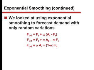
We lookedat using exponential
smoothing to forecast demand with
only random variations
Exponential Smoothing (continued)
Ft+1 = Ft + a (At - Ft)
Ft+1 = Ft + a At – a Ft
Ft+1 = a At + (1-a) Ft
62.
Exponential Smoothing (continued)
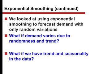
We looked at using exponential
smoothing to forecast demand with
only random variations
What if demand varies due to
randomness and trend?
What if we have trend and seasonality
in the data?
63.
Regression Analysis asa Method for
Forecasting
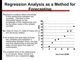
Regression analysis takes advantage
of the relationship between two
variables. Demand is then
forecasted based on the
knowledge of this relationship and
for the given value of the related
variable.
Ex: Sale of Tires (Y), Sale of Autos (X)
are obviously related
If we analyze the past data of these
two variables and establish a
relationship between them, we may
use that relationship to forecast the
sales of tires given the sales of
automobiles.
The simplest form of the relationship
is, of course, linear, hence it is
referred to as a regression line.
Sales of Autos (100,000)
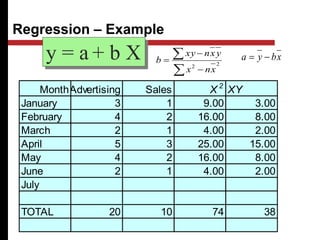
MonthAdvertising Sales X2
XY
January 3 1 9.00 3.00
February 4 2 16.00 8.00
March 2 1 4.00 2.00
April 5 3 25.00 15.00
May 4 2 16.00 8.00
June 2 1 4.00 2.00
July
TOTAL 20 10 74 38
y = a + b X
Regression – Example
2
2
x
n
x
y
x
n
xy
b x
b
y
a
66.
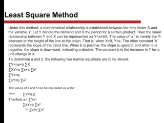
Least Square Method
Underthis method, a mathematical relationship is established between the time factor X and
the variable Y. Let Y denote the demand and X the period for a certain product. Then the linear
relationship between Y and X can be represented as Y=a+bX. The value of ‘a ‘ is merely the Y-
intercept or the height of the line at the origin. That is, when X=0, Y=a. The other constant ‘b’
represents the slope of the trend line. When b is positive, the slope is upward, and when b is
negative, the slope is downward, indicating a decline. The constant b is the increase in Y for a
unit change in X.
To determine a and b, the following two normal equations are to be sloved:
∑Y=na+b ∑X
∑XY=a ∑x+b ∑x2
∑Y=na
∑xY=b ∑x2
The values of a and b can be calculated as under:
Since ∑Y=n.a
Therfore a= ∑Y/n
∑xY=b ∑x2
b= ∑xY/ ∑x2
67.
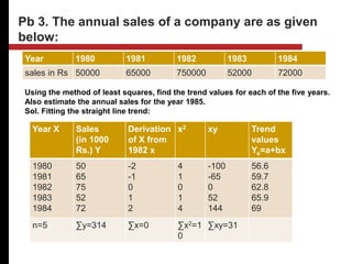
Using the methodof least squares, find the trend values for each of the five years.
Also estimate the annual sales for the year 1985.
Sol. Fitting the straight line trend:
Year 1980 1981 1982 1983 1984
sales in Rs 50000 65000 750000 52000 72000
Pb 3. The annual sales of a company are as given
below:
Year X Sales
(in 1000
Rs.) Y
Derivation
of X from
1982 x
x2 xy Trend
values
Ye=a+bx
1980
1981
1982
1983
1984
50
65
75
52
72
-2
-1
0
1
2
4
1
0
1
4
-100
-65
0
52
144
56.6
59.7
62.8
65.9
69
n=5 ∑y=314 ∑x=0 ∑x2=1
0
∑xy=31
68.
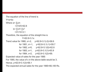
The equation ofthe line of trend is
Y=a+bx
Where a= ∑y/n
=314/5=62.8
b= ∑xY/ ∑x2
=31/10=3.1
Therefore, the equation of the straight line is
Y=62.8+3.1x
Trend value for 1980, x=-2, y=62.8+3.1(-2)=56.6
for 1981, x=-1, y=62.8+3.1(-1)=59.7
for 1982, x=0, y=62.8+3.1(0)=62.8
for 1983, x=1, y=62.8+3.1(1)=65.9
for 1984, x=2, y=62.8+3.1(2)=69.
Expected value of sales for the year 1985
For 1985, the value of x in the above table would be 3.
Hence, y=62.8+3.1(3)=66.1
The expected annual sales for the year 1985=66,100 Rs.
69.
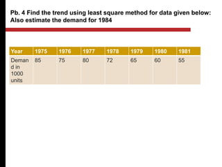
Pb. 4 Findthe trend using least square method for data given below:
Also estimate the demand for 1984
Year 1975 1976 1977 1978 1979 1980 1981
Deman
d in
1000
units
85 75 80 72 65 60 55
70.
Now, a= ∑y/n=492/7=70.285
b=∑αy/ ∑x2 =-135/28=-4.822
The line of best fit is
Y=a=bx=70.825+(-4.822)x
Trend for the year 1984.
Now for the year 1984, x=7
Y=70.825+(-4.822)×7=40.531 units.
Year X Sales (in
1000 Rs.)
Y
Deviation
of X from
1978 x
x2 xy Trend
values
Ye =a+bx
1975
1976
1977
1978
1979
1980
1981
n=7
85
75
80
72
65
60
55
∑y=192
-3
-2
-1
0
1
2
3
∑x=0
9
4
1
0
1
4
9
∑x2 =28
-255
-150
-80
0
65
120
165
∑xy=-135


![Product1 [3] forecasting v2](https://cdn.slidesharecdn.com/ss_thumbnails/product13-forecastingv2-190226041012-thumbnail.jpg?width=640&height=640&fit=bounds)


