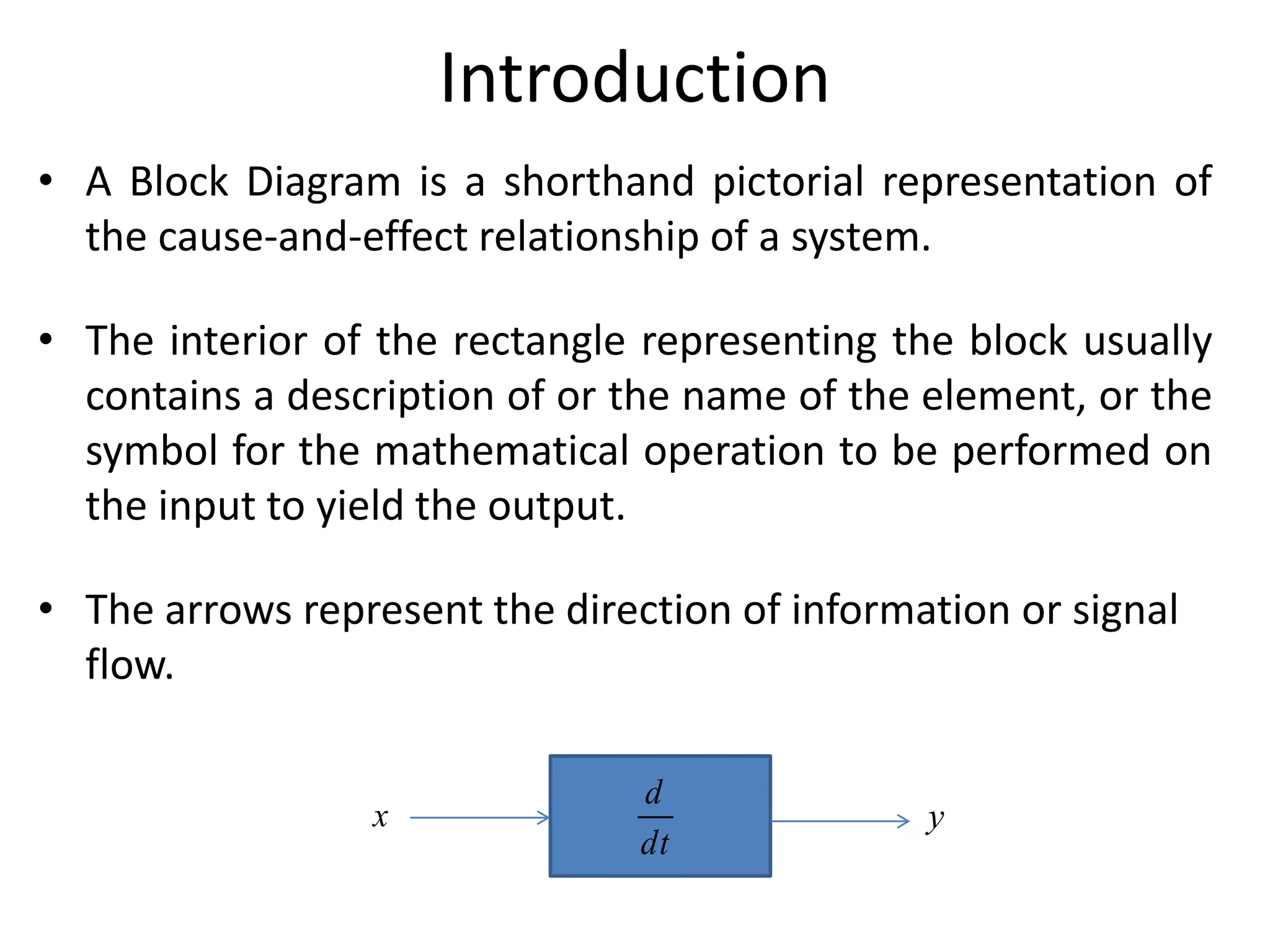
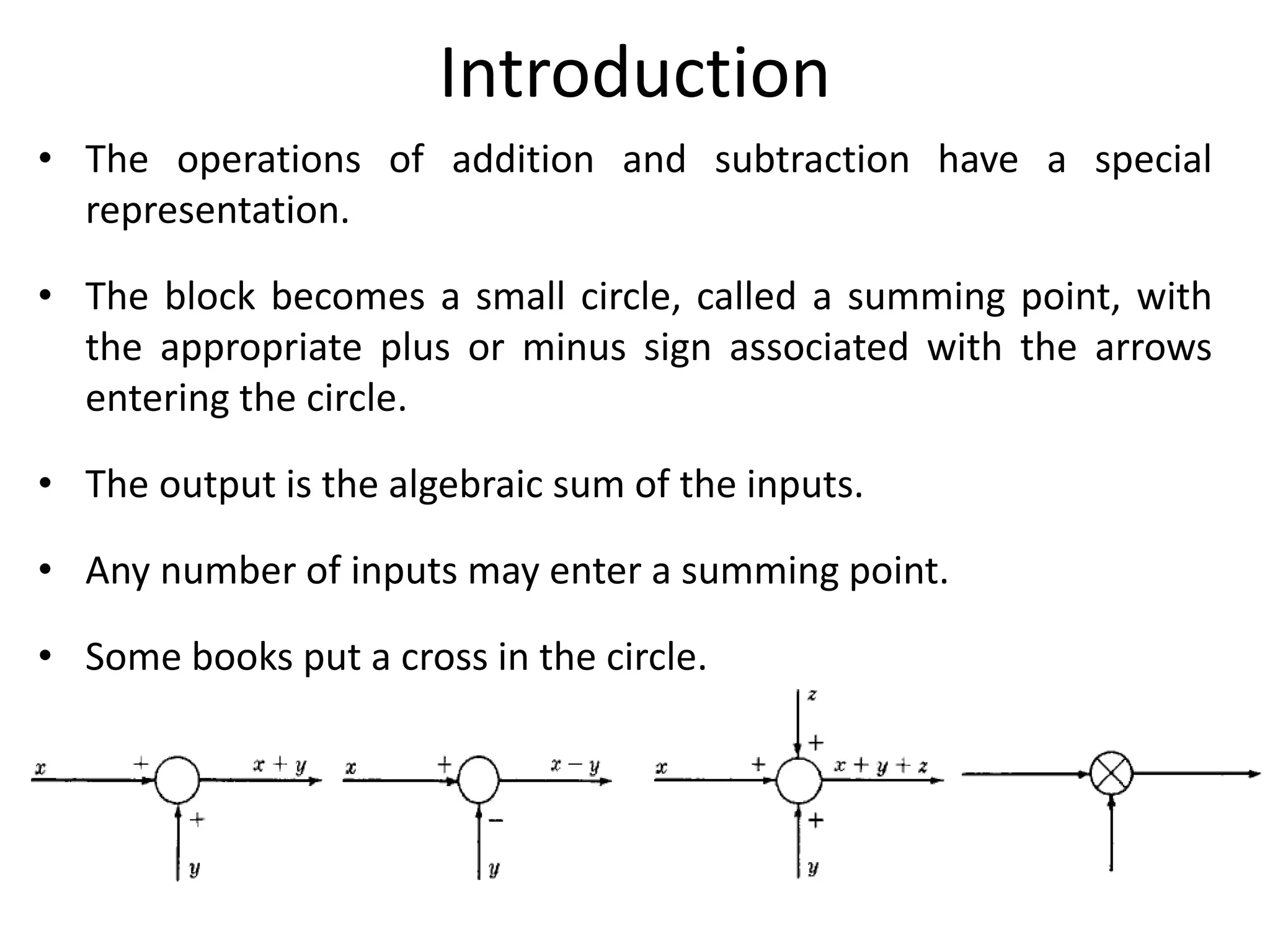
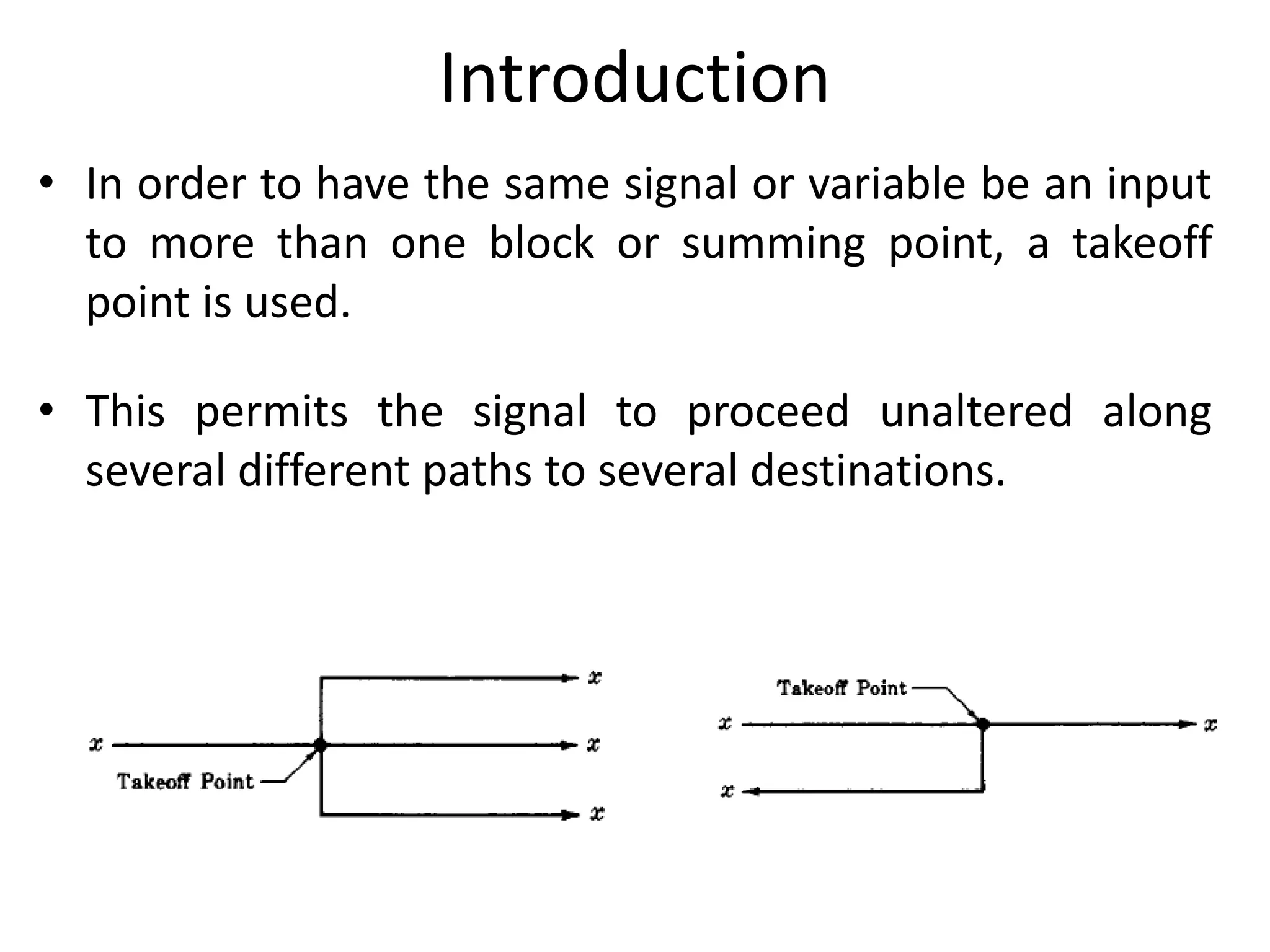
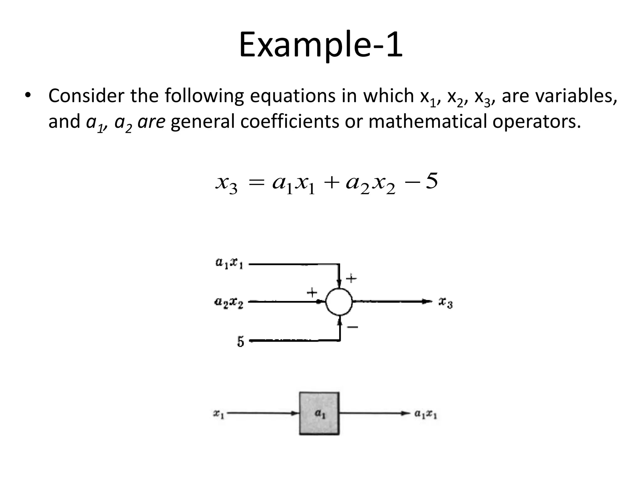
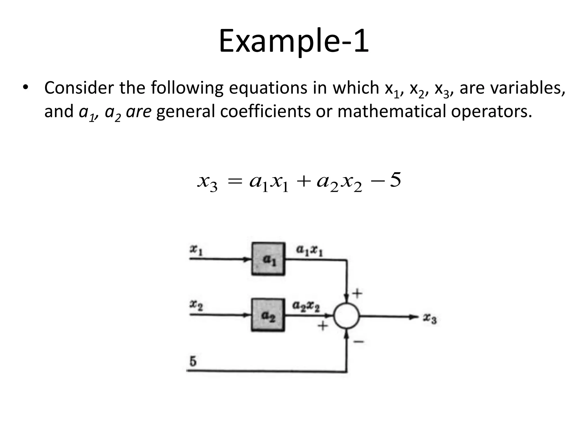
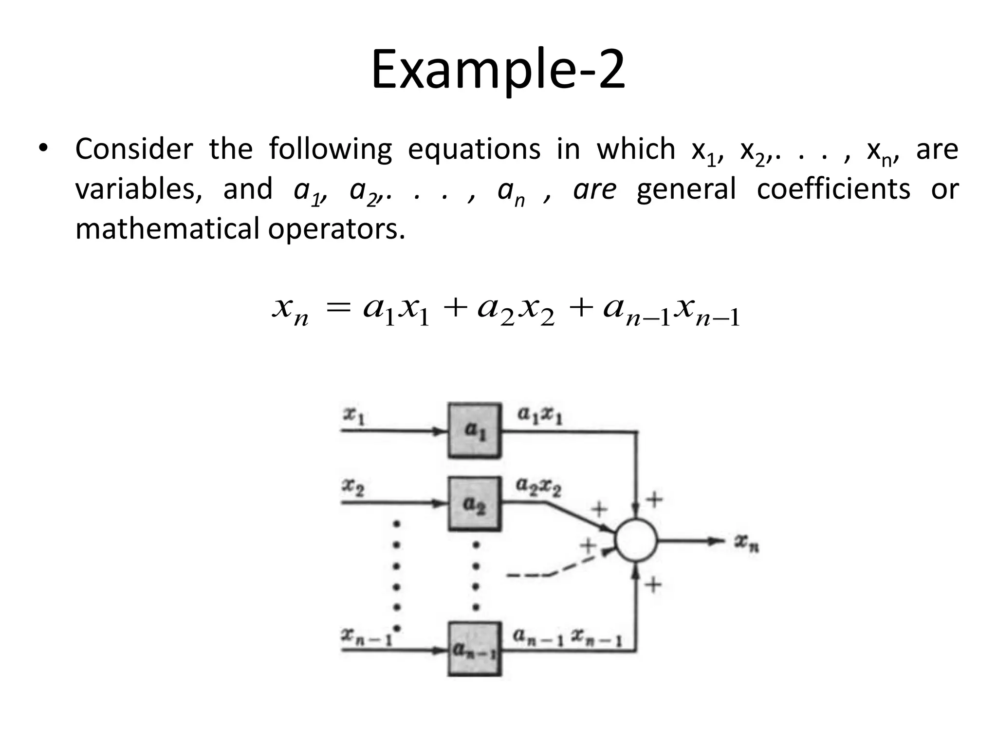
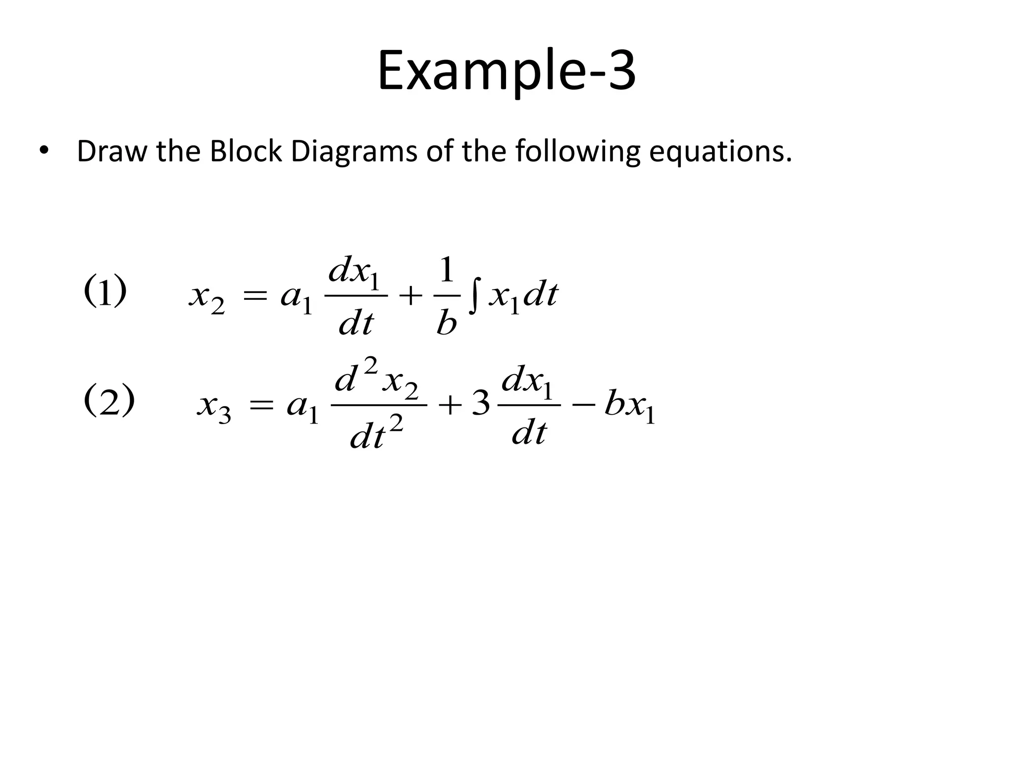
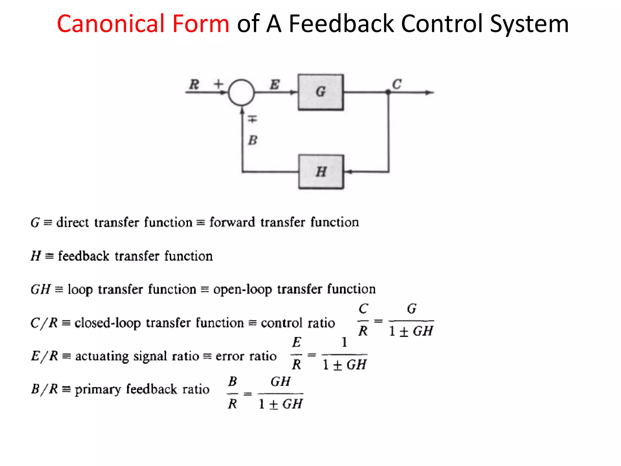
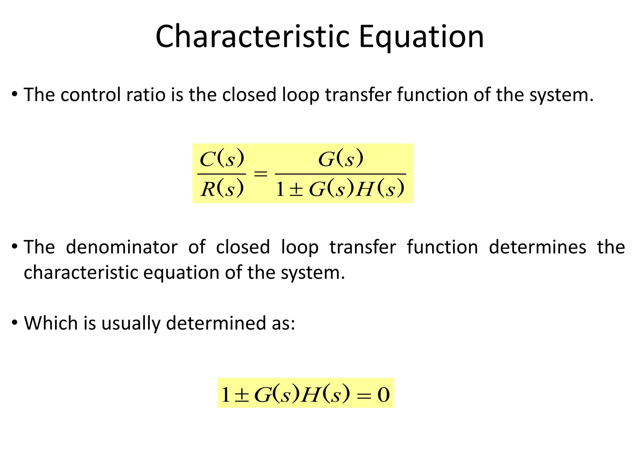
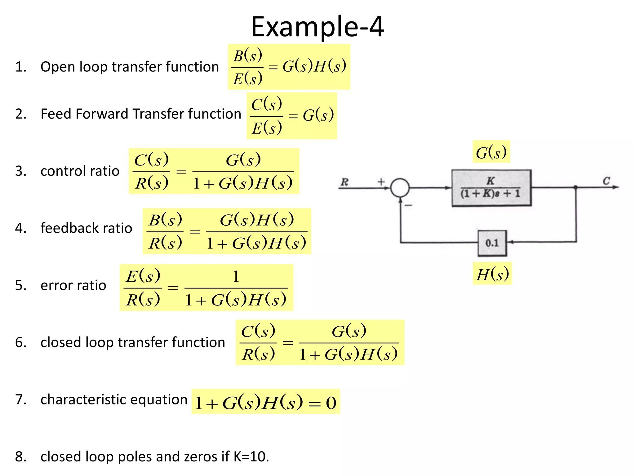
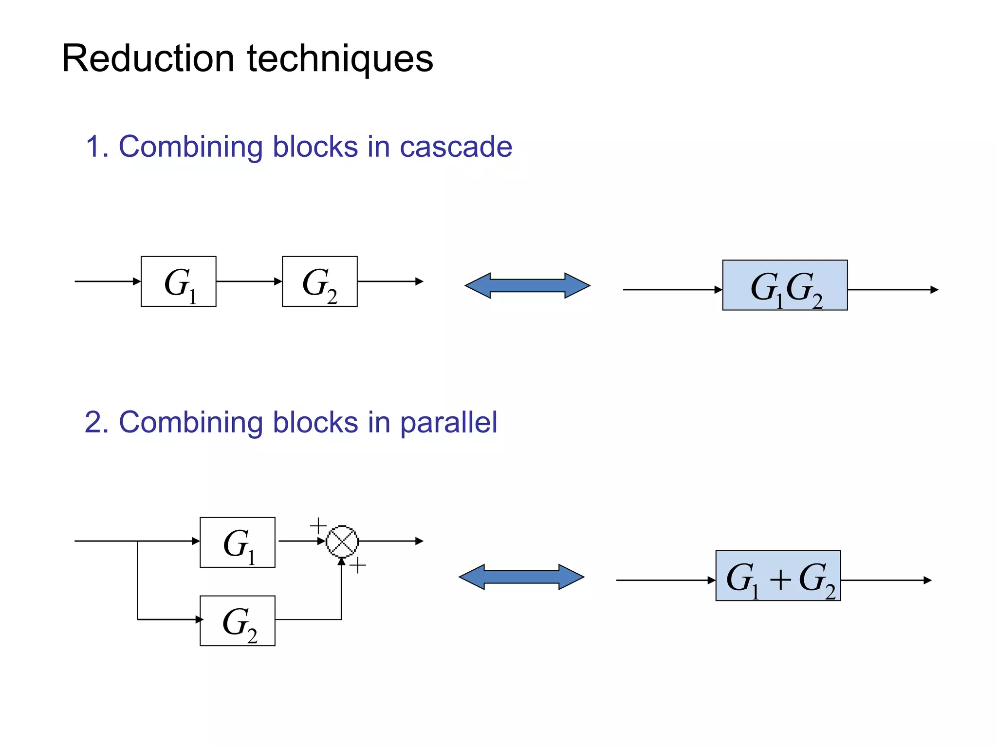
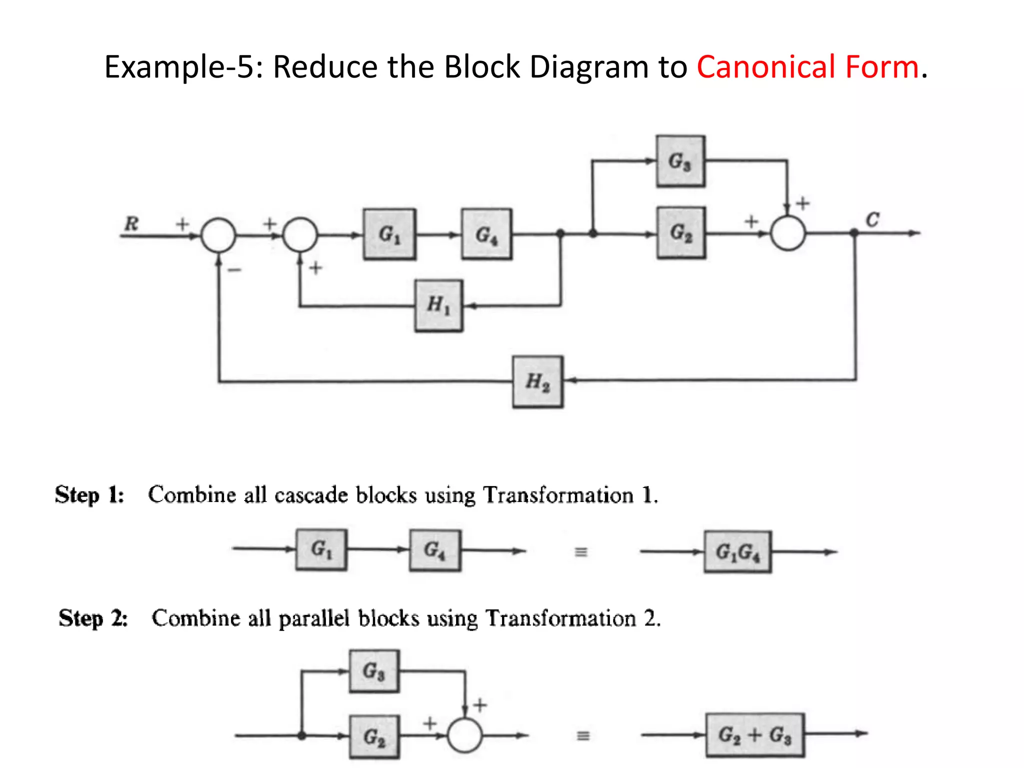
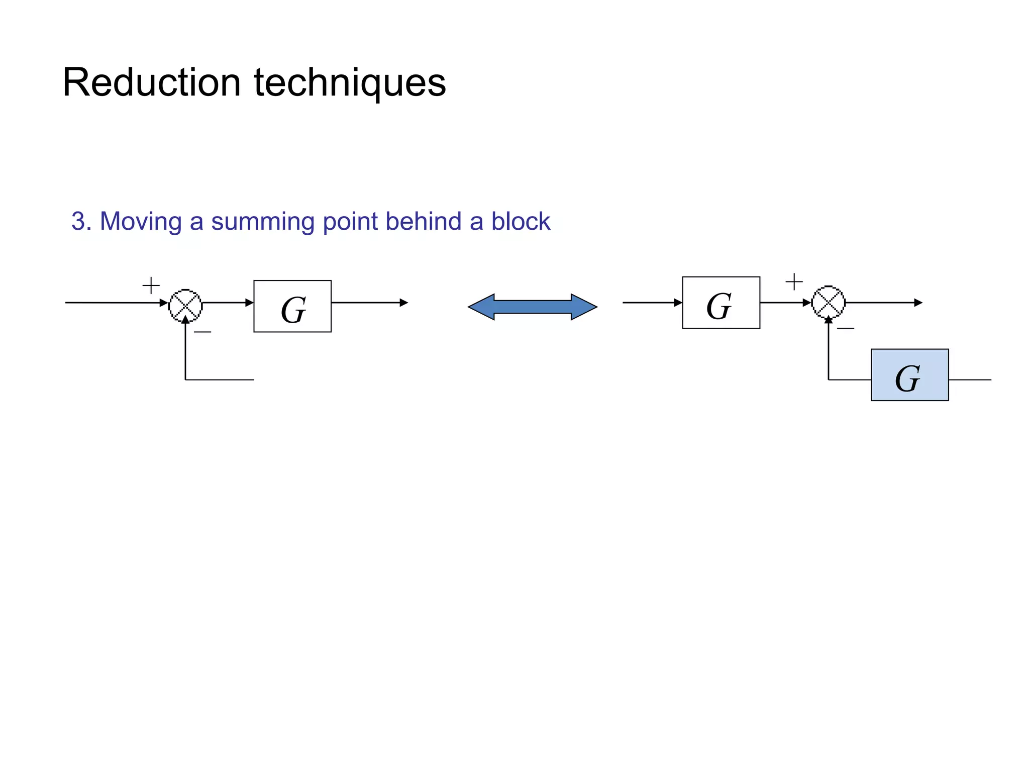
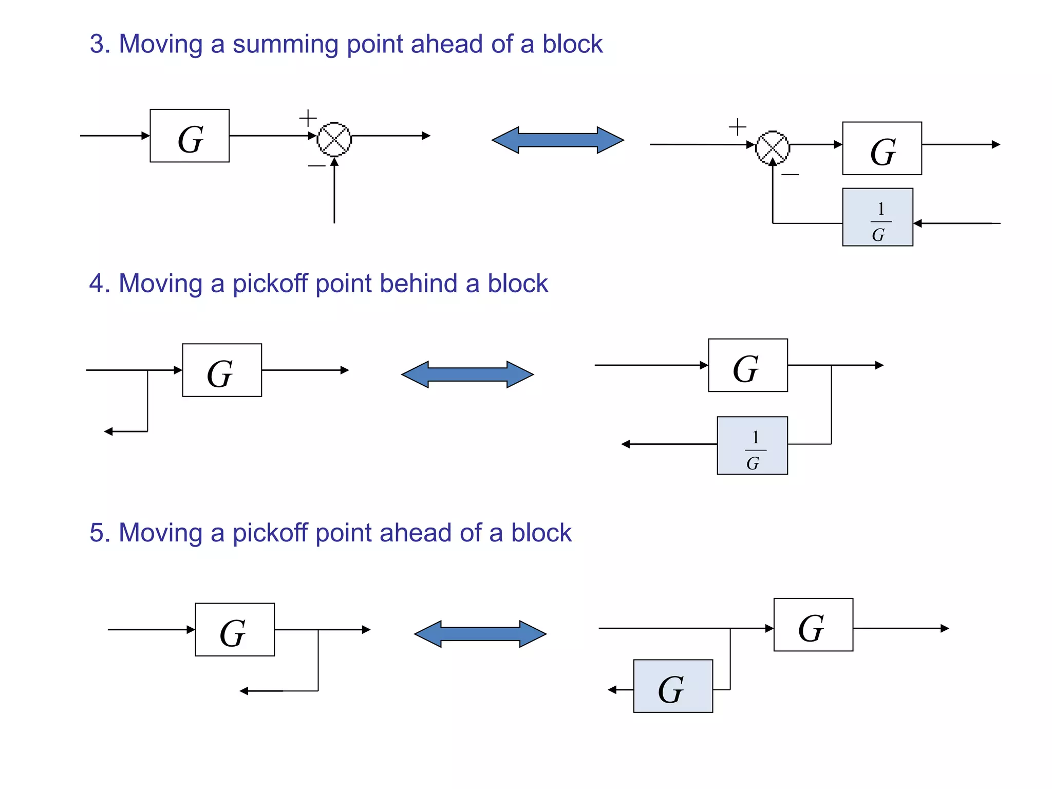
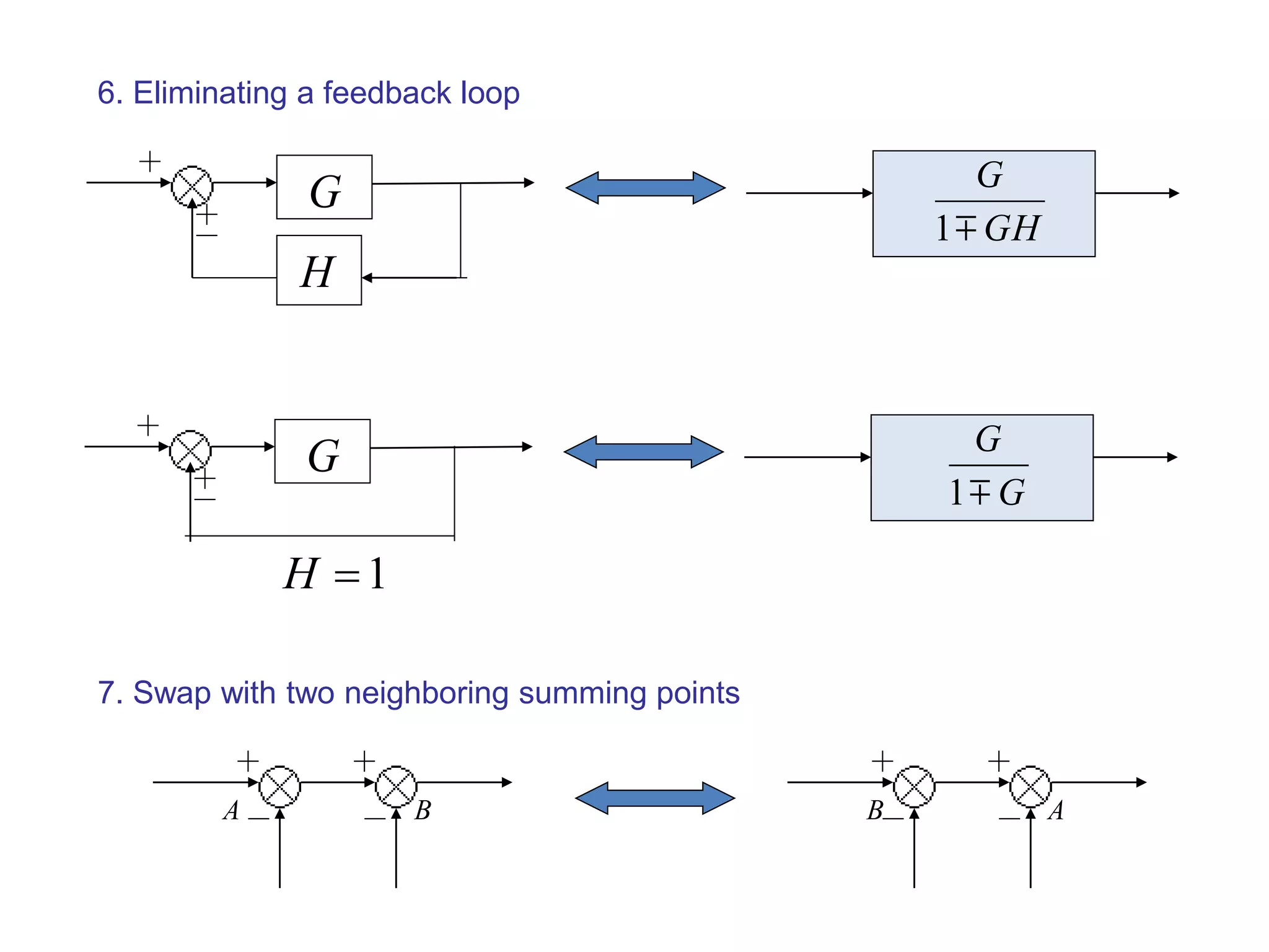
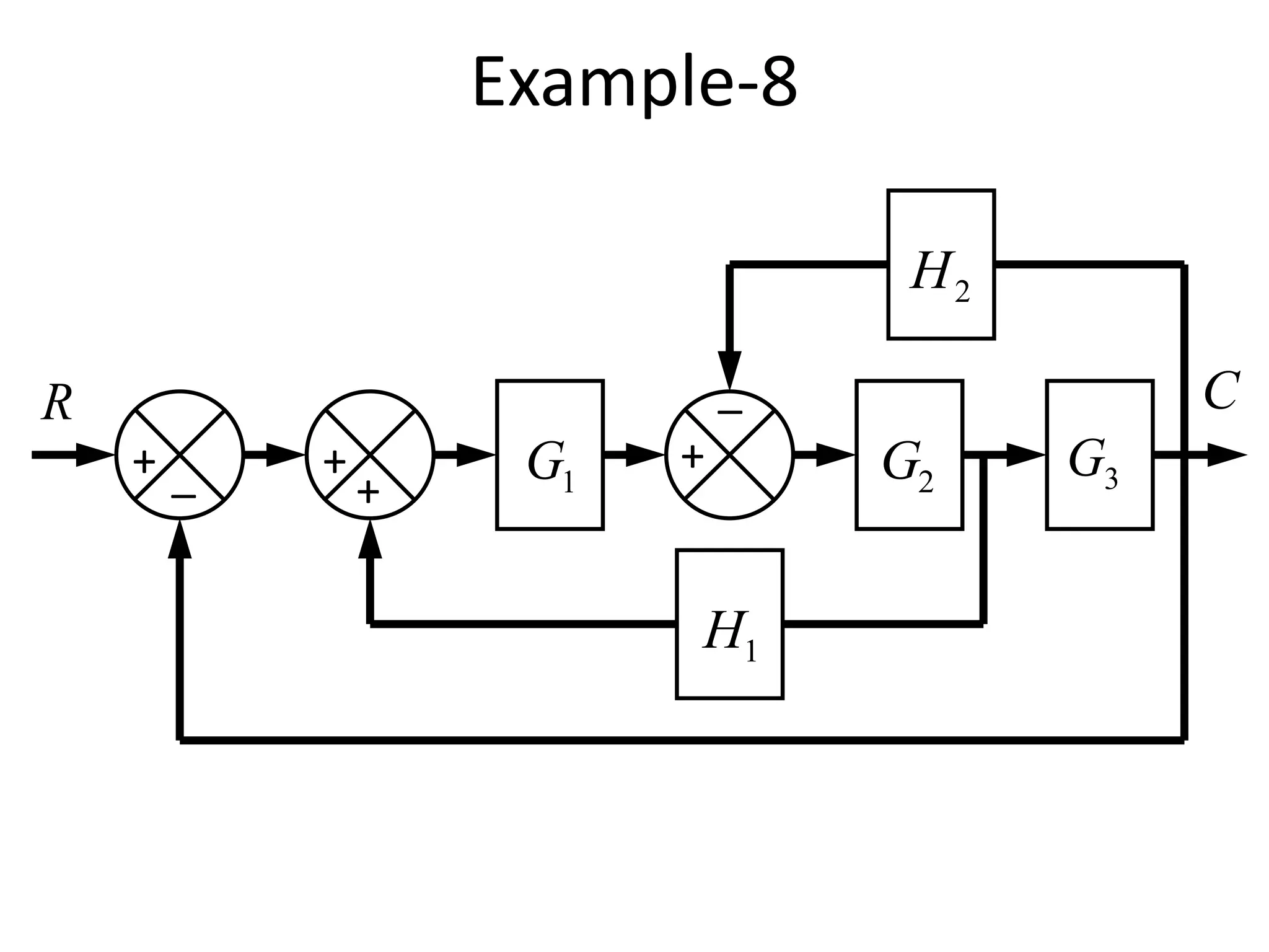
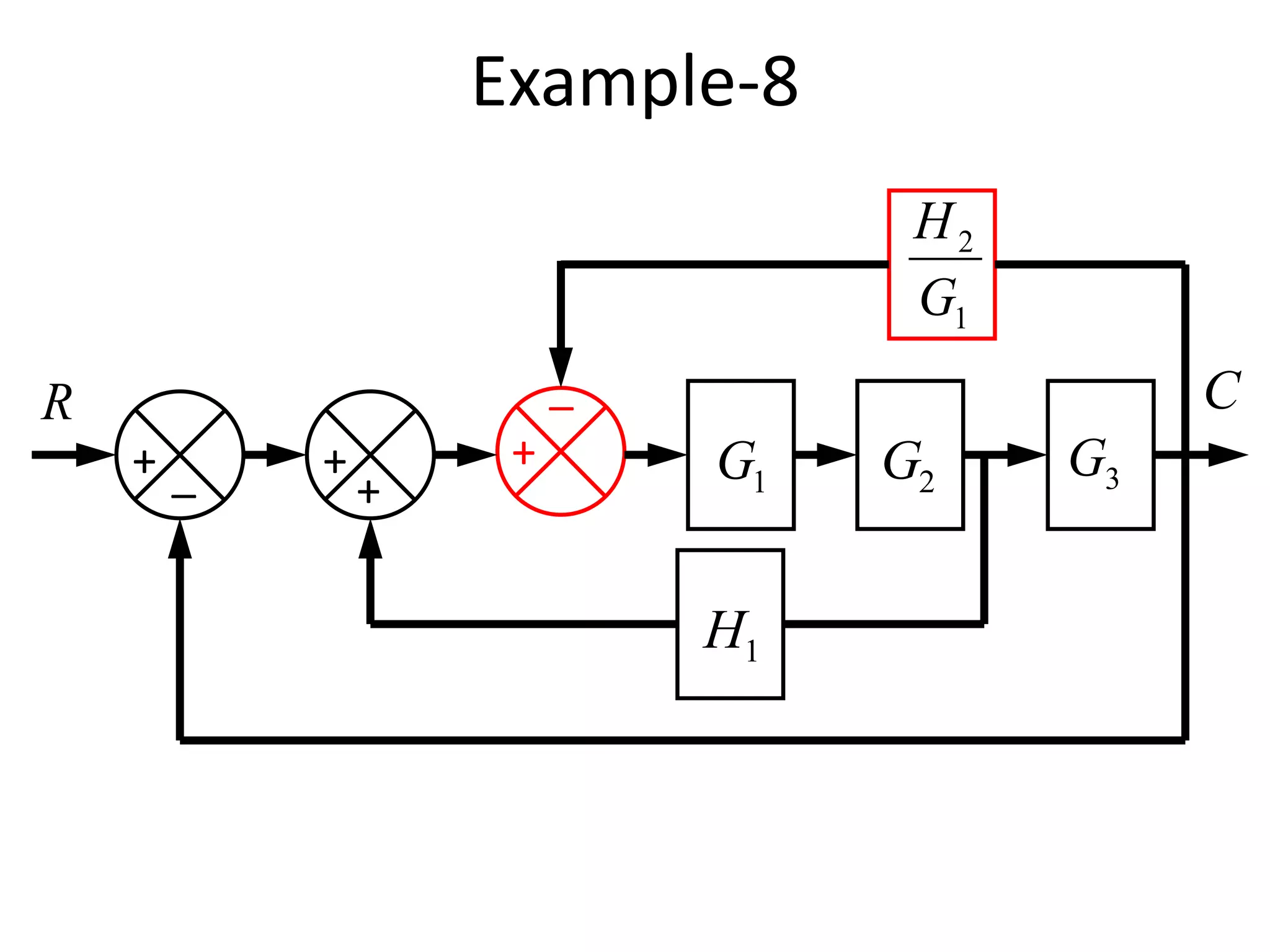
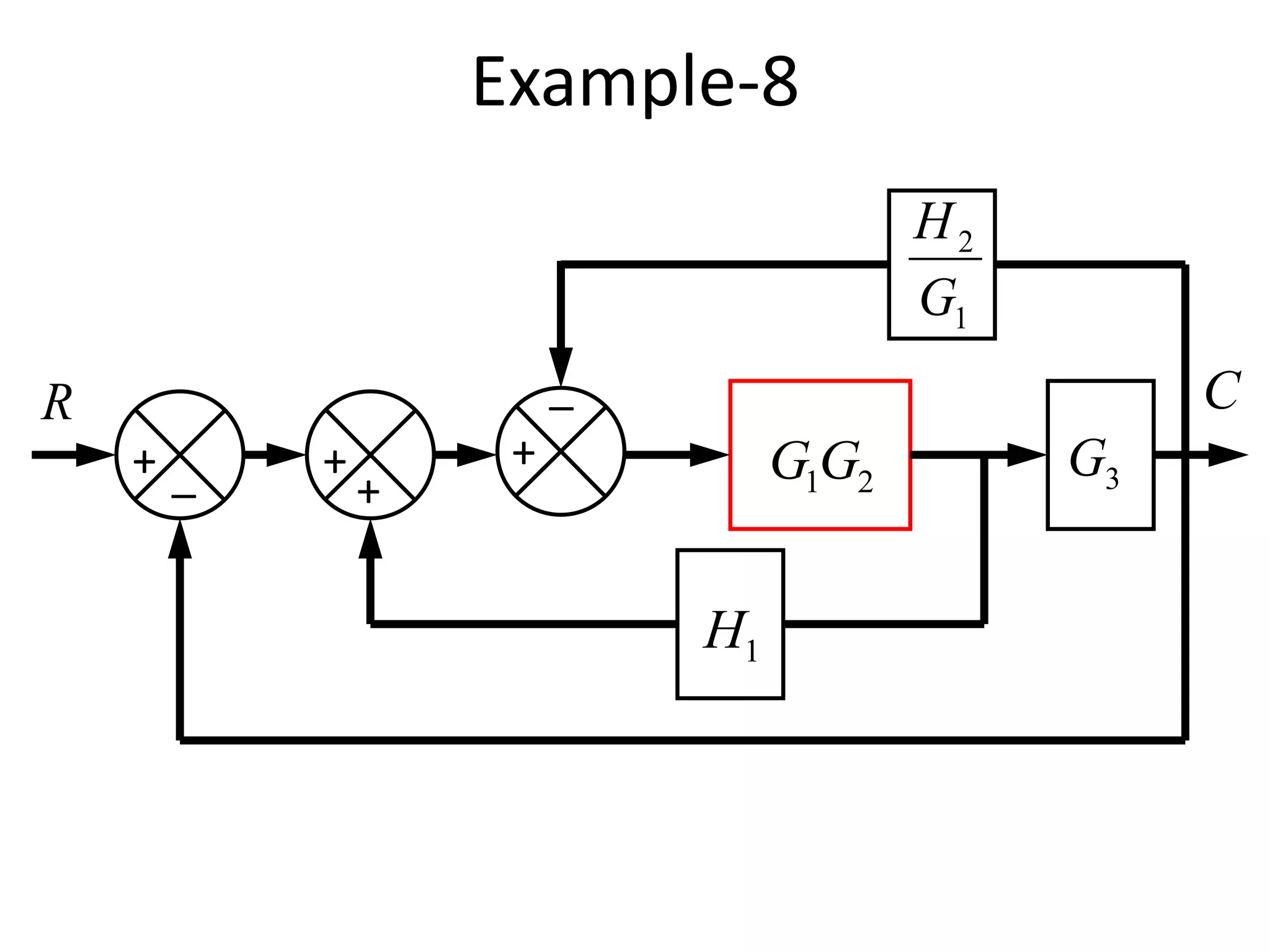
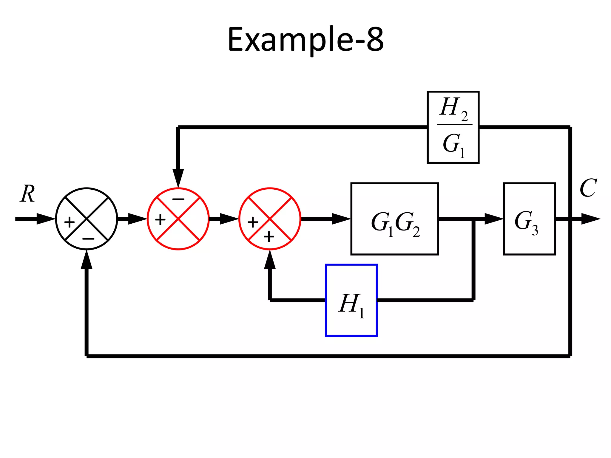
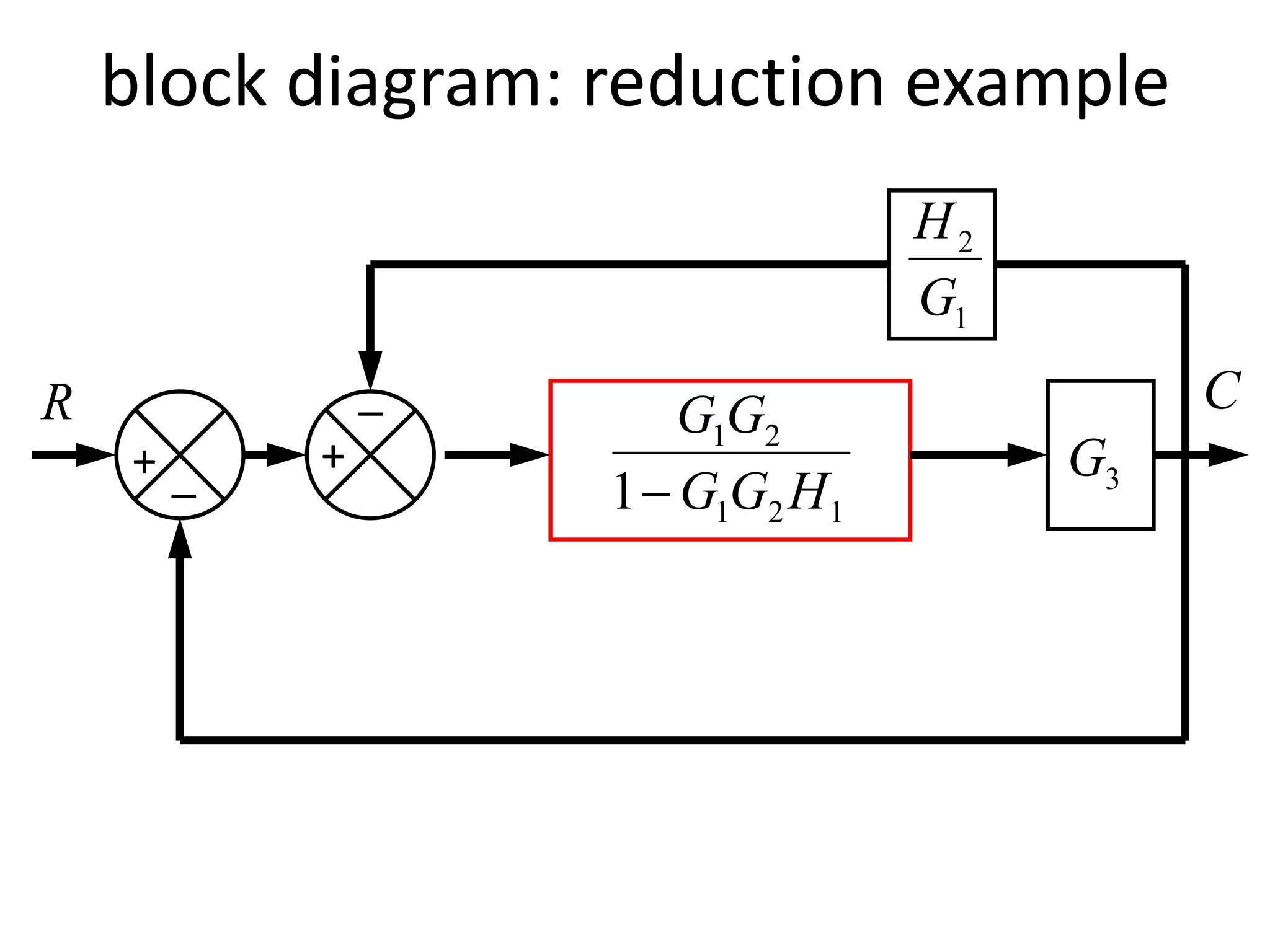
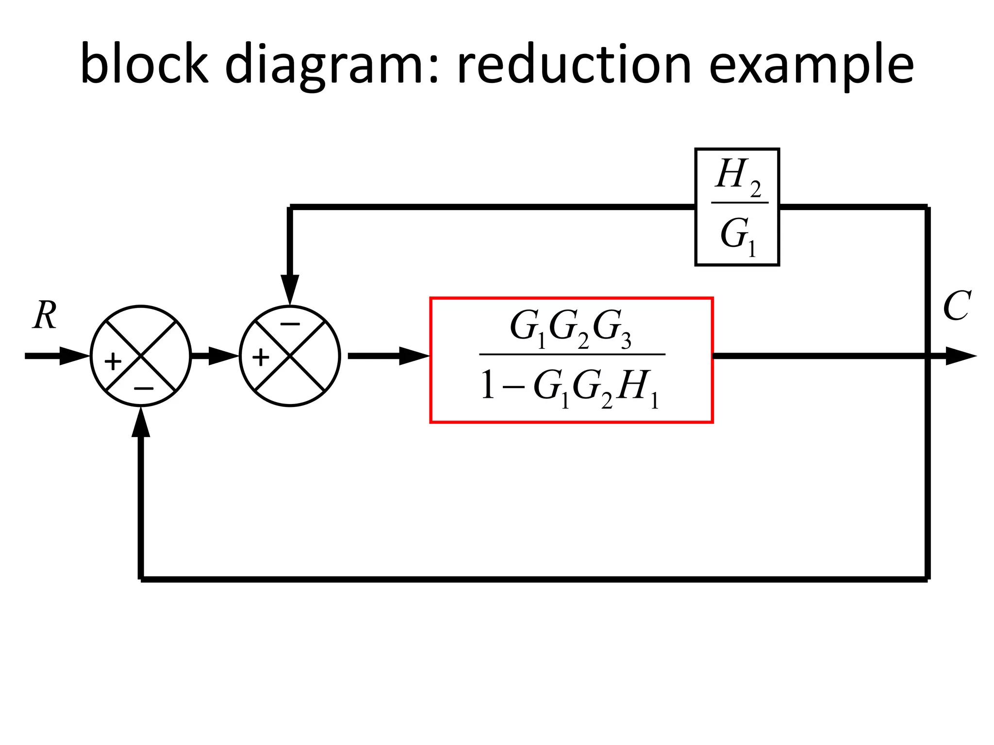
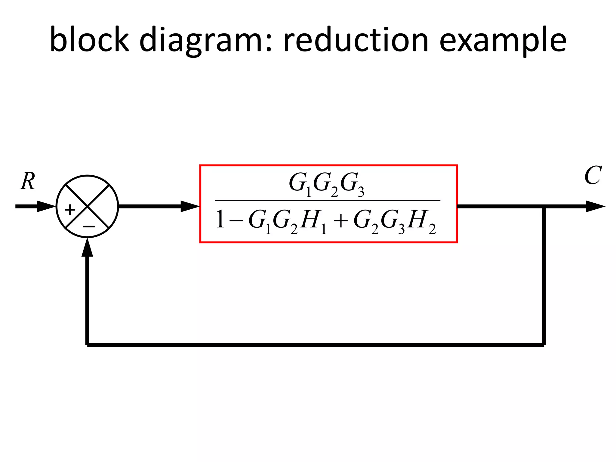
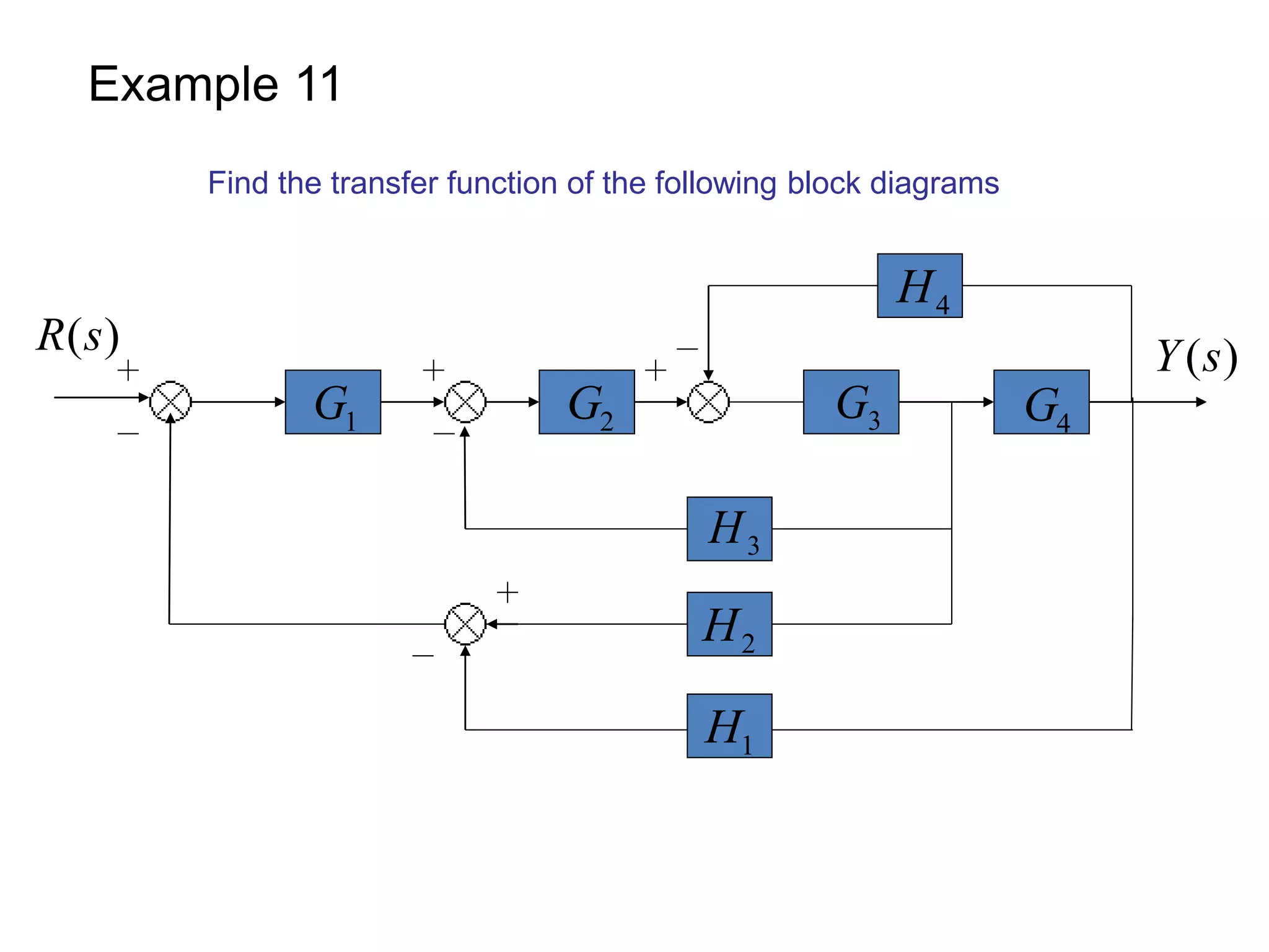
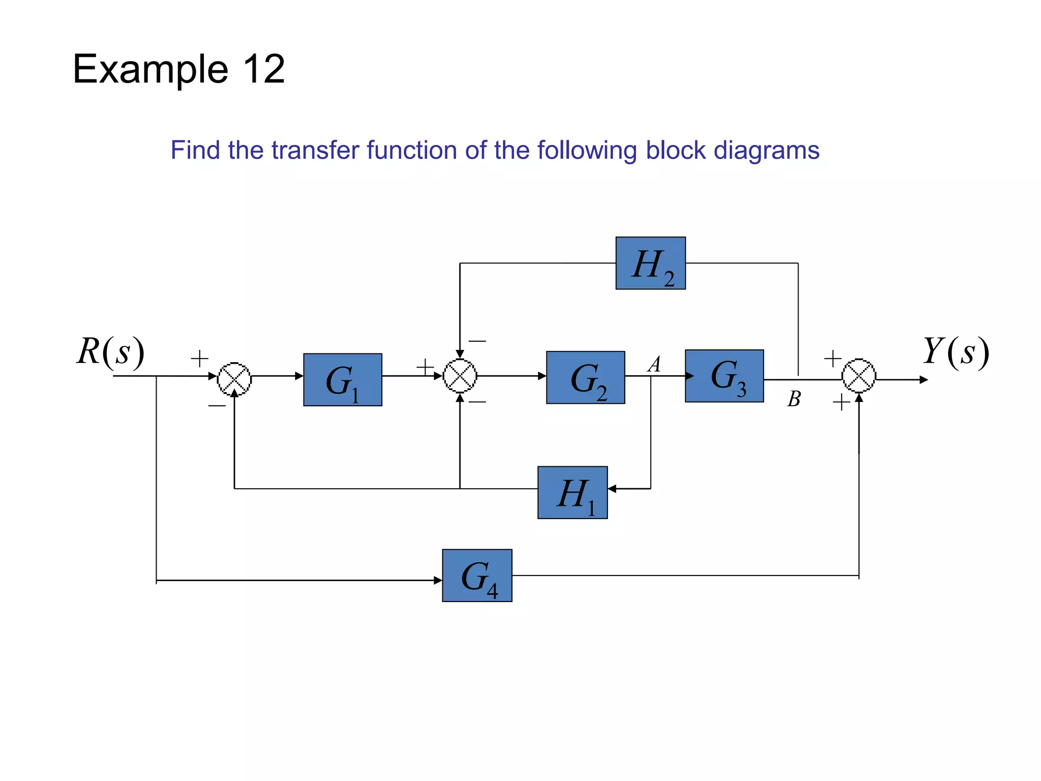
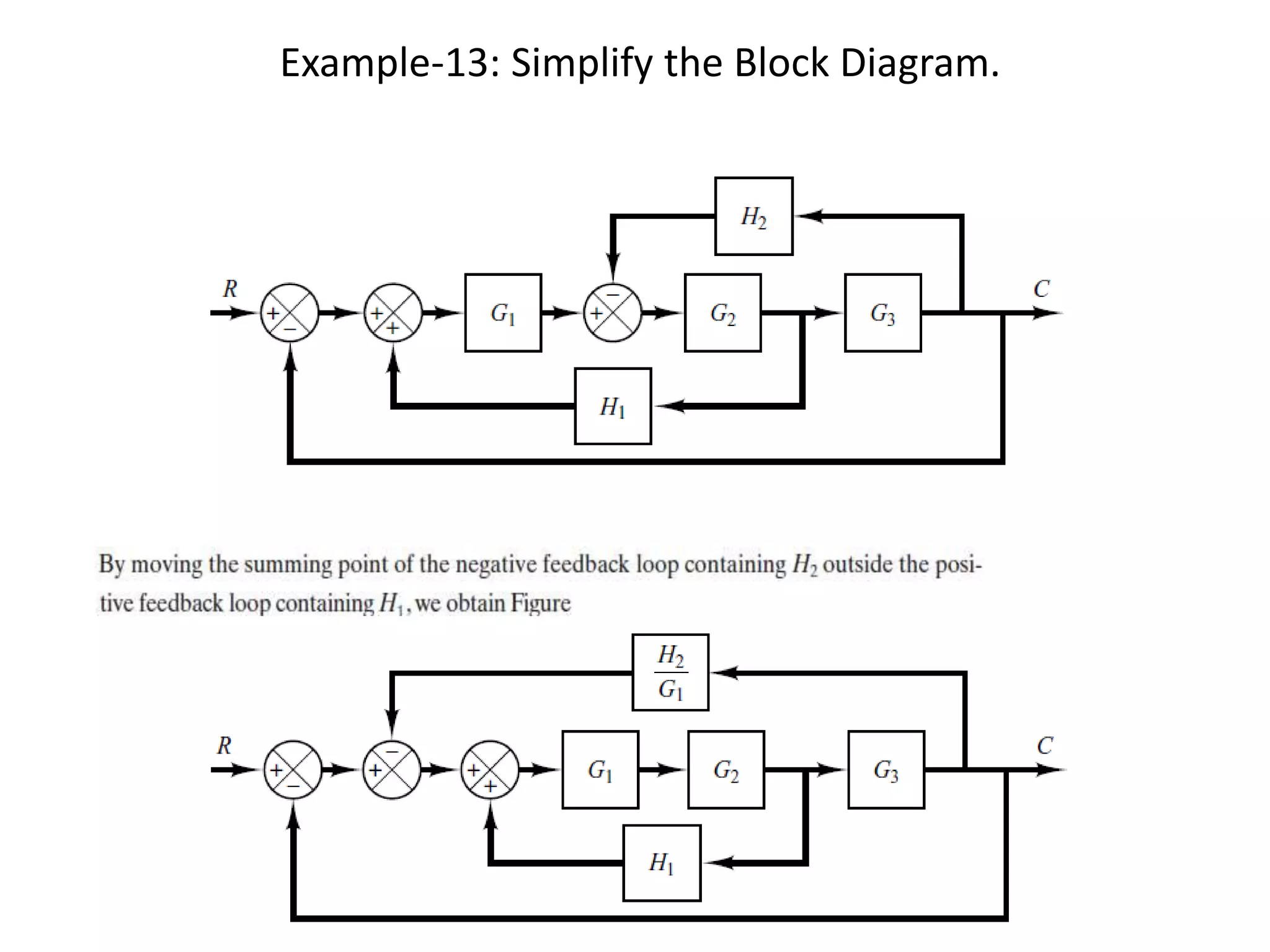
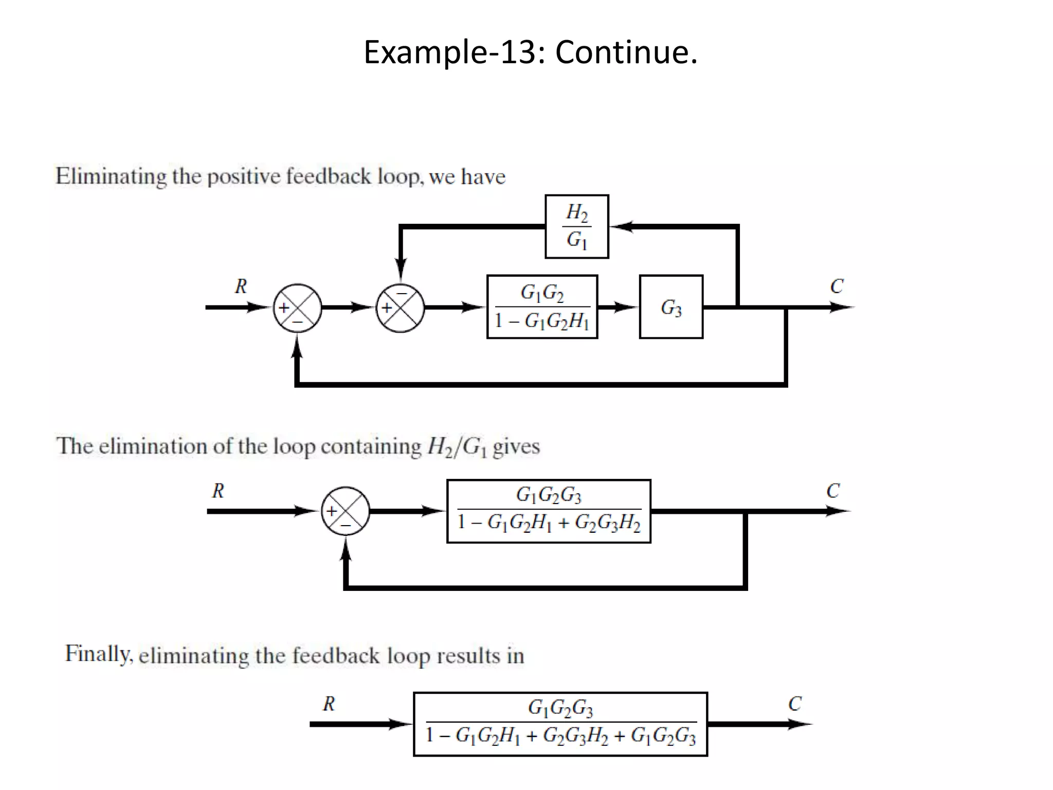
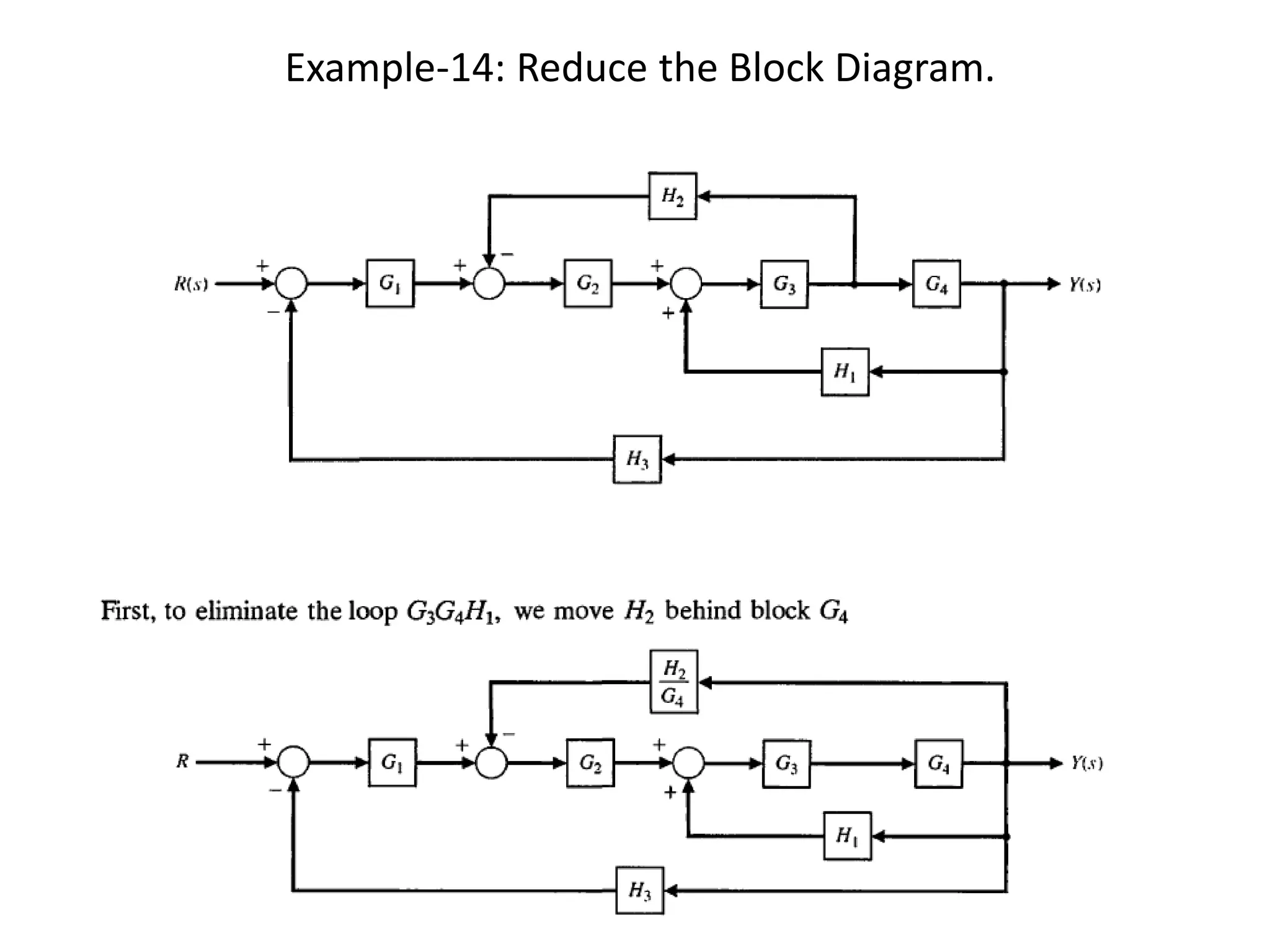
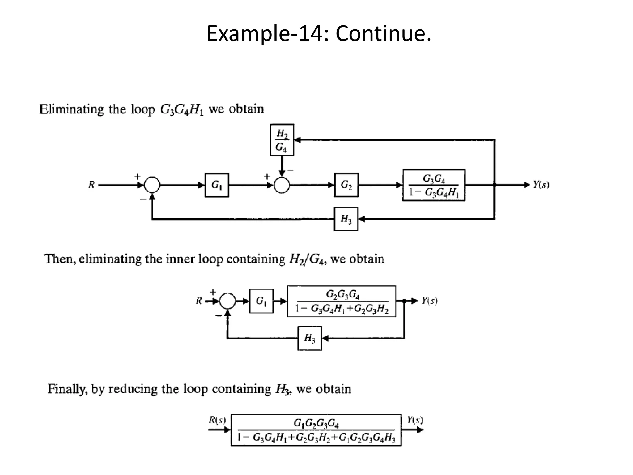
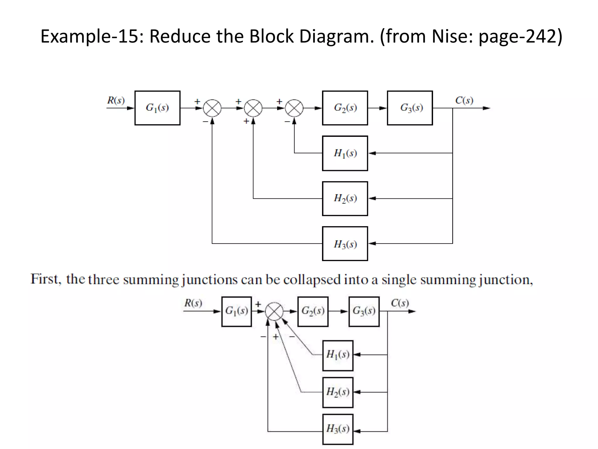
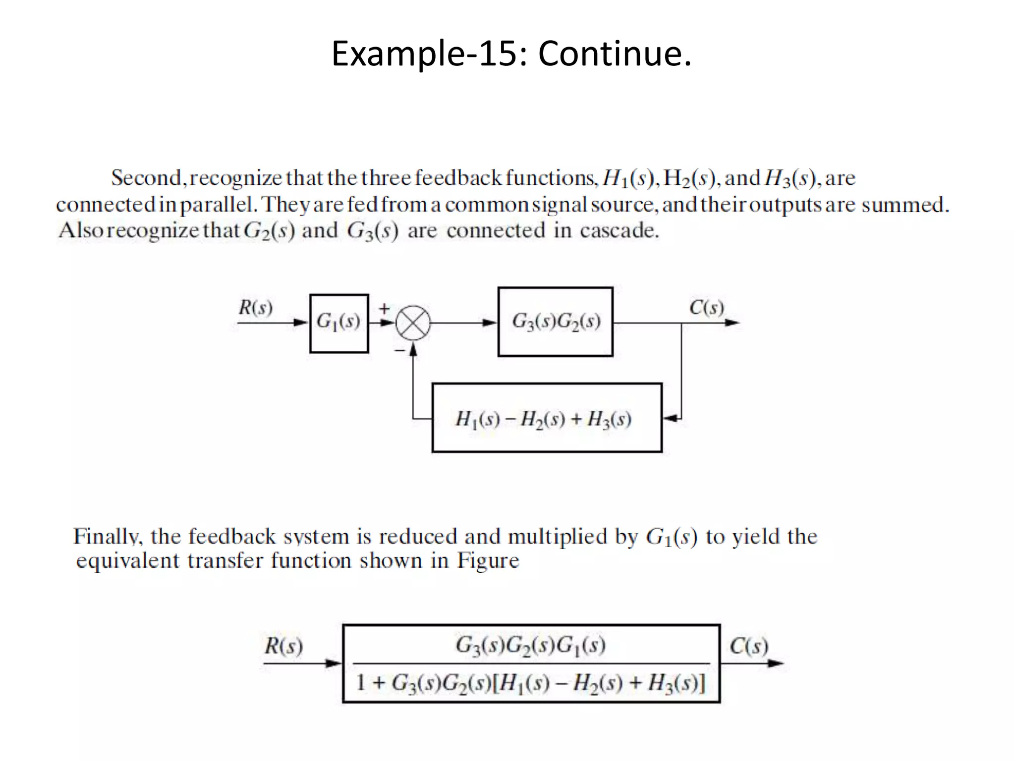
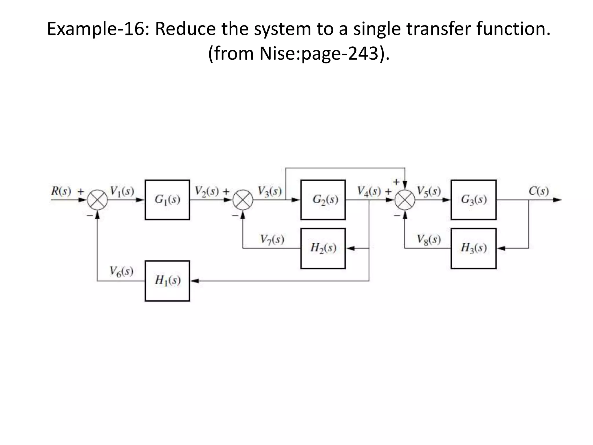
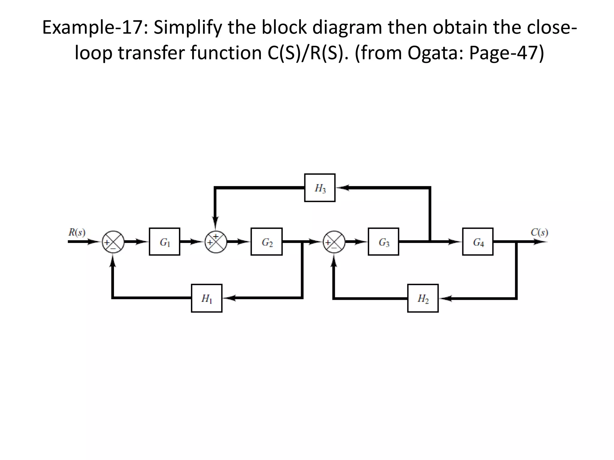
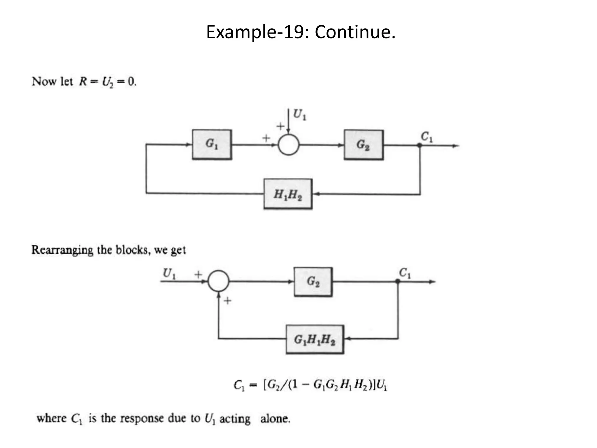
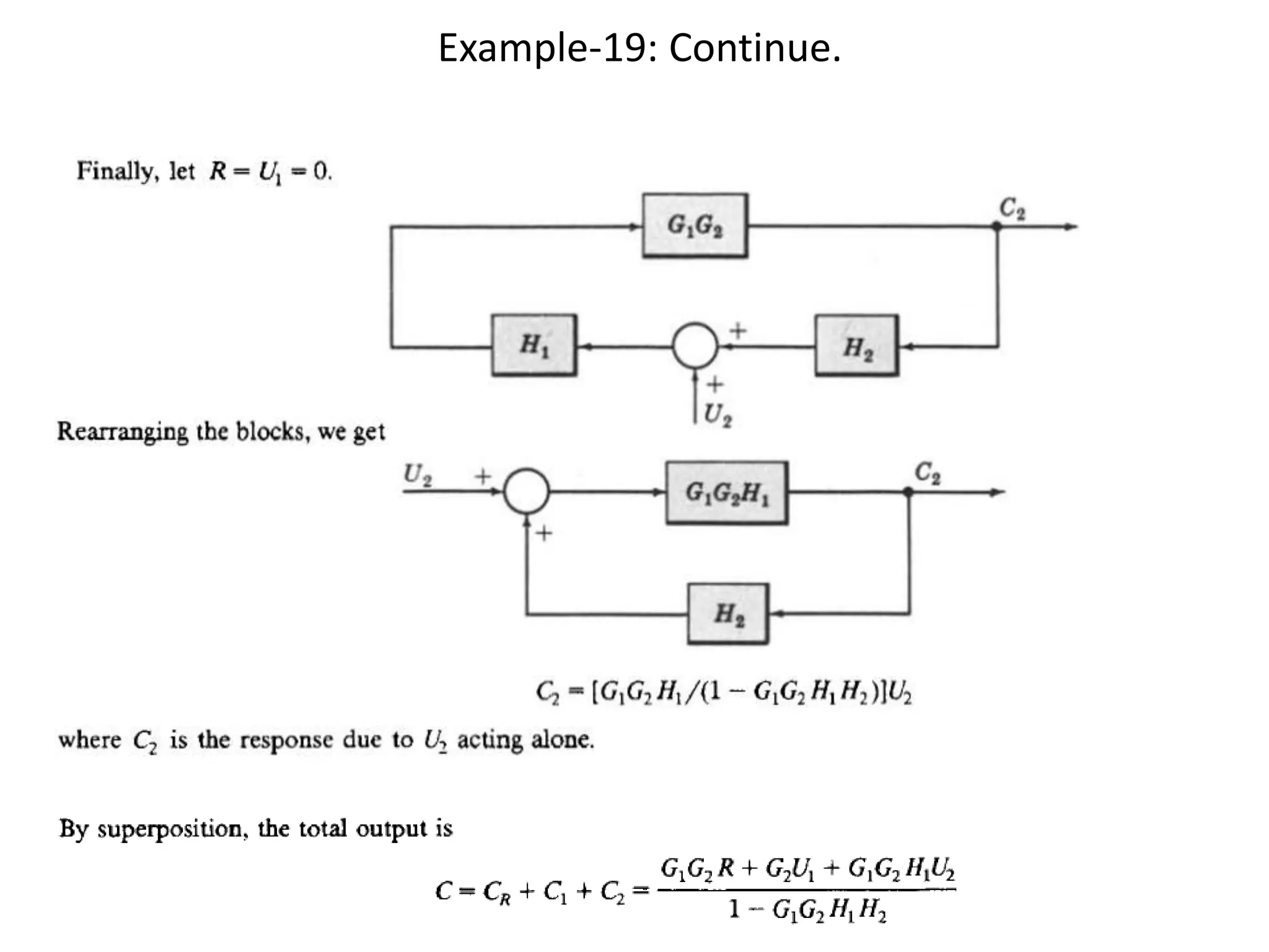
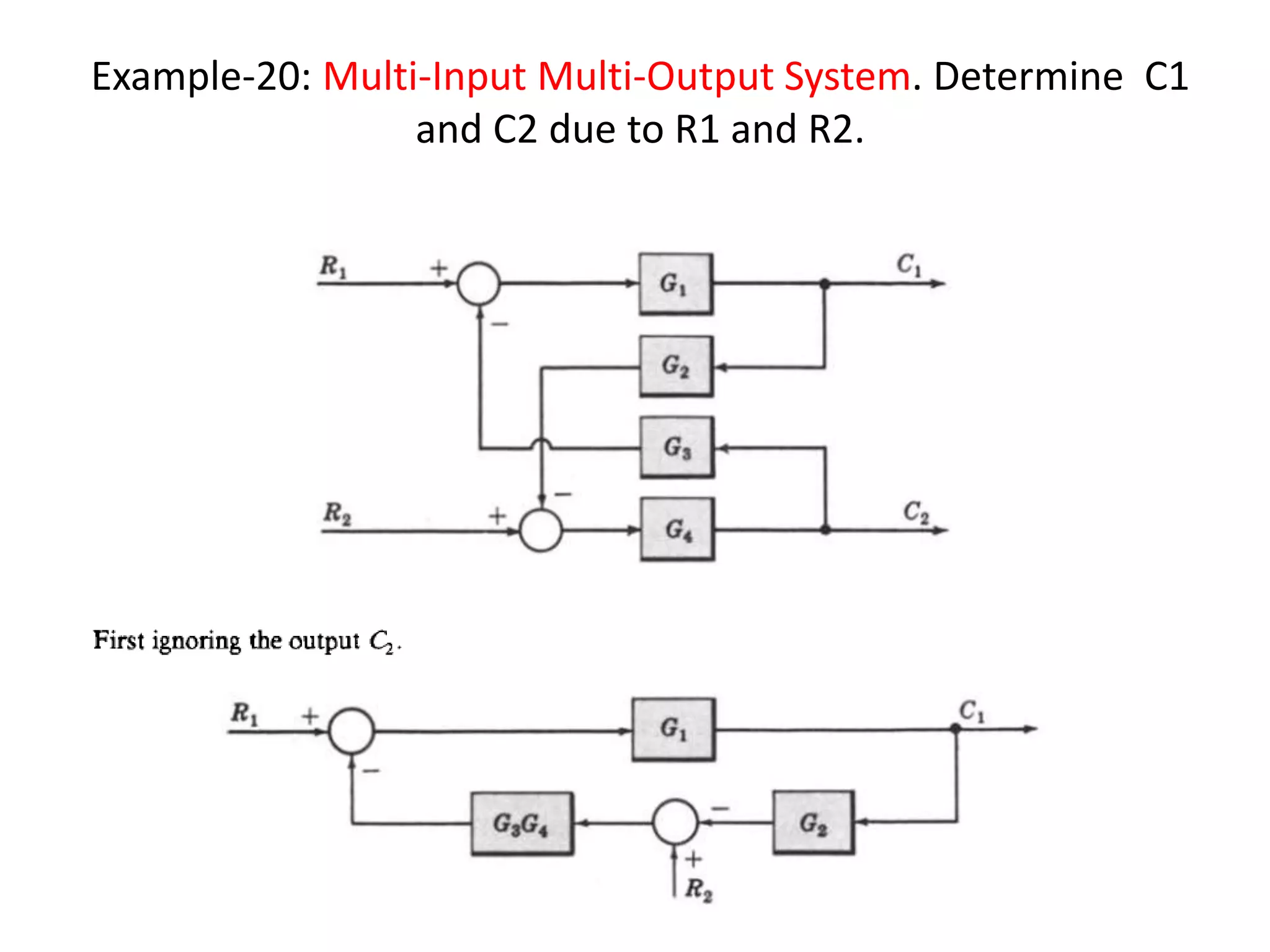
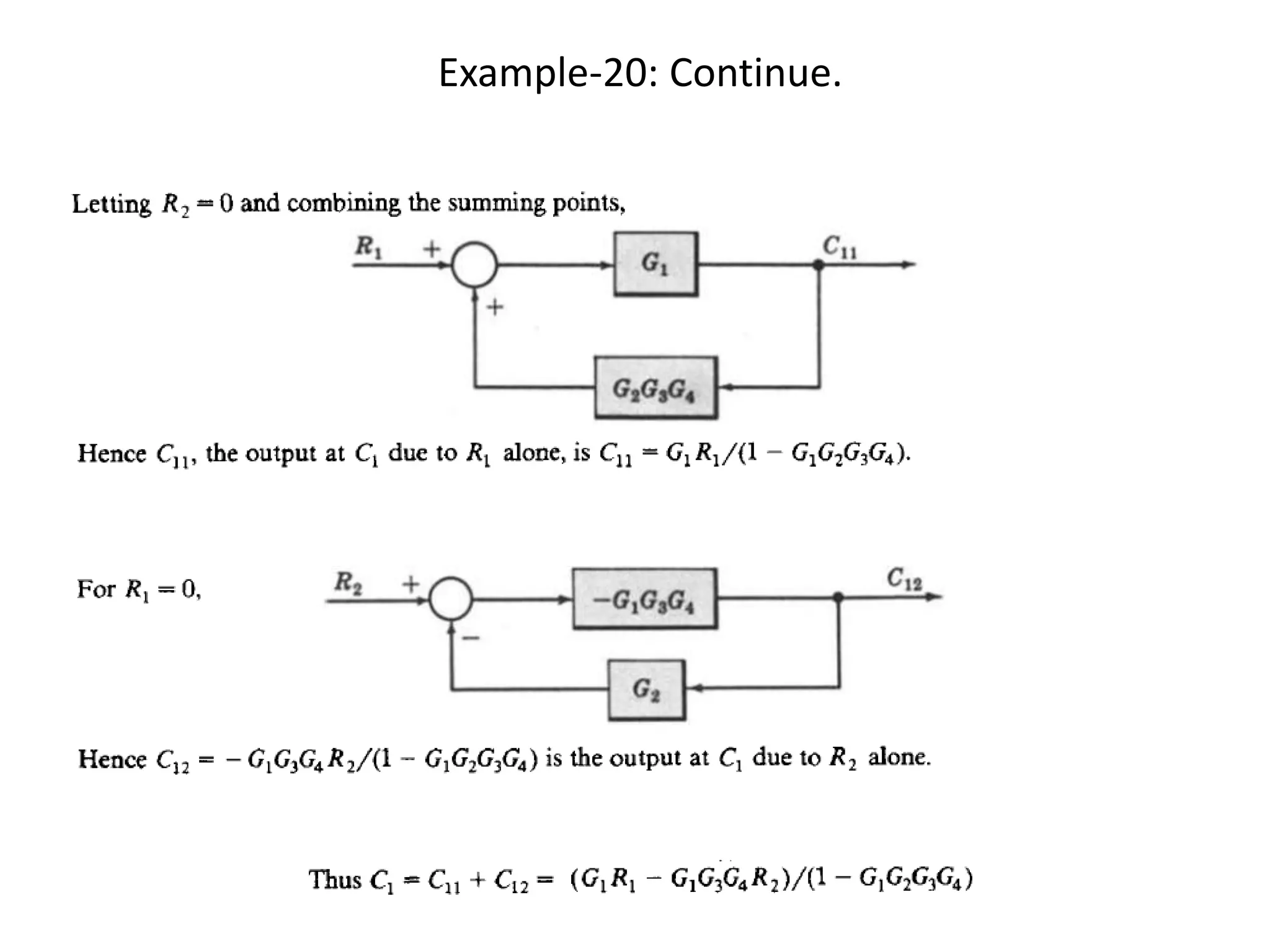
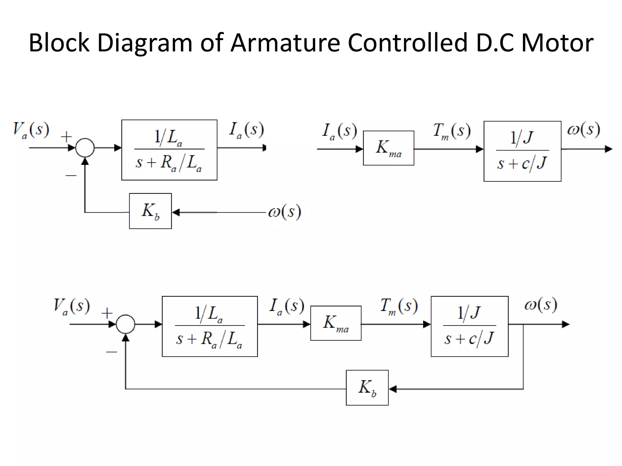
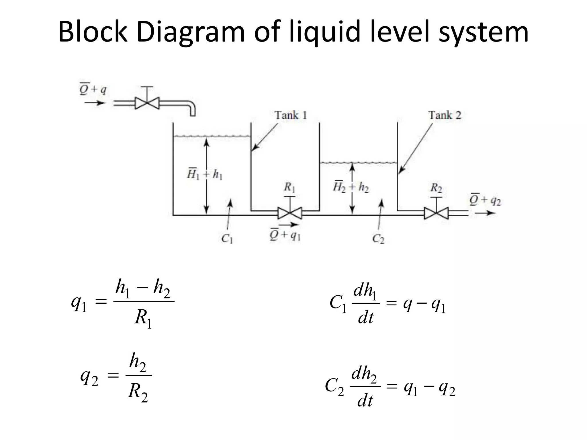
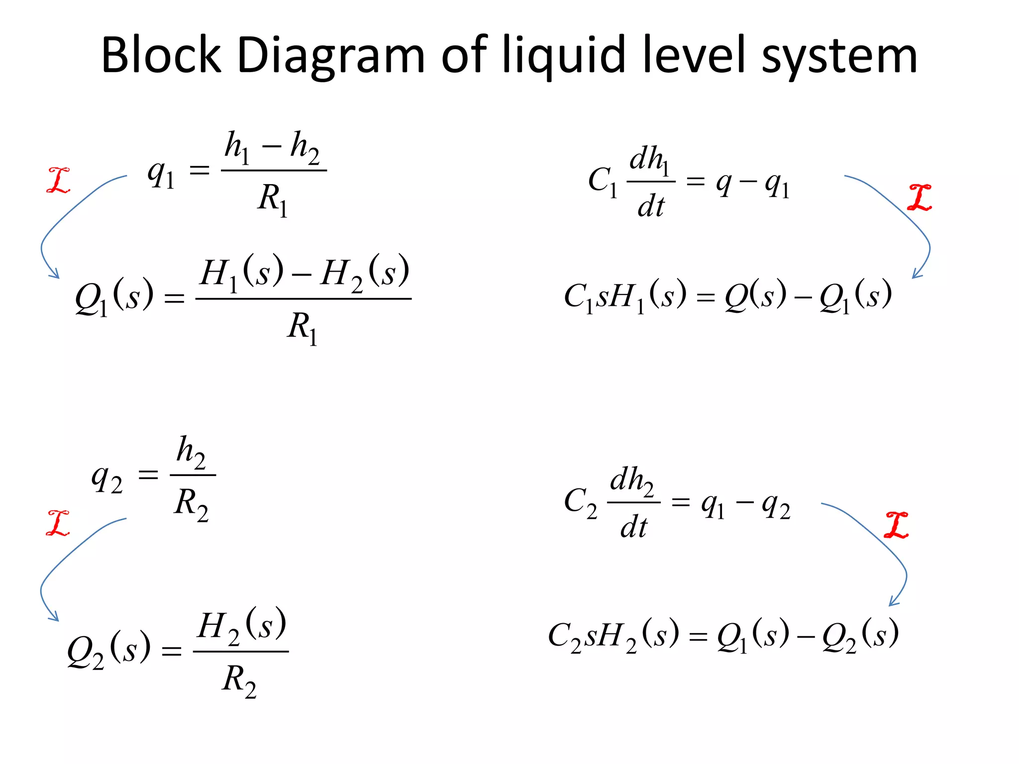
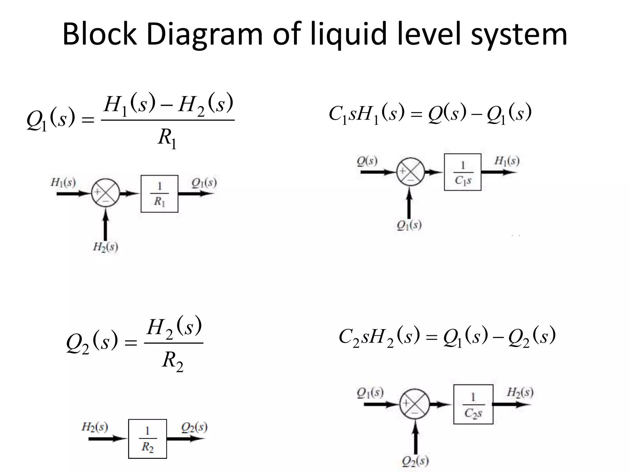
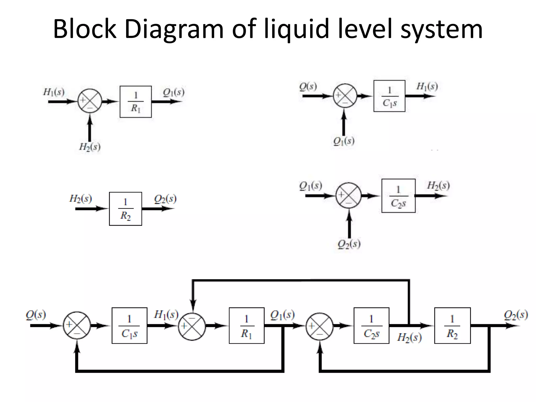
This document provides an introduction to block diagram representation of control systems. It discusses how block diagrams provide a pictorial representation of the relationships between elements in a system using blocks and arrows. The blocks represent system elements or operations, and the arrows represent the direction of signal or information flow. Specific topics covered include summing points, takeoff points, examples of representing equations as block diagrams, and canonical forms.

1. Feedback Control Systems (FCS)
Dr. Imtiaz Hussain
email: imtiaz.hussain@faculty.muet.edu.pk
URL :http://imtiazhussainkalwar.weebly.com/
Lecture-14-15
Block Diagram Representation of Control Systems

2. Introduction
• A Block Diagram is a shorthand pictorial representation of
the cause-and-effect relationship of a system.
• The interior of the rectangle representing the block usually
contains a description of or the name of the element, or the
symbol for the mathematical operation to be performed on
the input to yield the output.
• The arrows represent the direction of information or signal
flow.
dt
d
x y

3. Introduction
• The operations of addition and subtraction have a special
representation.
• The block becomes a small circle, called a summing point, with
the appropriate plus or minus sign associated with the arrows
entering the circle.
• The output is the algebraic sum of the inputs.
• Any number of inputs may enter a summing point.
• Some books put a cross in the circle.

4. Introduction
• In order to have the same signal or variable be an input
to more than one block or summing point, a takeoff
point is used.
• This permits the signal to proceed unaltered along
several different paths to several destinations.

5. Example-1
• Consider the following equations in which x1, x2, x3, are variables,
and a1, a2 are general coefficients or mathematical operators.
522113  xaxax

6. Example-1
• Consider the following equations in which x1, x2, x3, are variables,
and a1, a2 are general coefficients or mathematical operators.
522113  xaxax

7. Example-2
• Consider the following equations in which x1, x2,. . . , xn, are
variables, and a1, a2,. . . , an , are general coefficients or
mathematical operators.
112211  nnn xaxaxax

8. Example-3
• Draw the Block Diagrams of the following equations.
1
1
2
2
2
13
1
1
12
32
1
1
bx
dt
dx
dt
xd
ax
dtx
bdt
dx
ax


)(
)(

9. Canonical Form of A Feedback Control System

10. Characteristic Equation
• The control ratio is the closed loop transfer function of the system.
• The denominator of closed loop transfer function determines the
characteristic equation of the system.
• Which is usually determined as:
)()(
)(
)(
)(
sHsG
sG
sR
sC


1
01  )()( sHsG

11. Example-4
1. Open loop transfer function
2. Feed Forward Transfer function
3. control ratio
4. feedback ratio
5. error ratio
6. closed loop transfer function
7. characteristic equation
8. closed loop poles and zeros if K=10.
)()(
)(
)(
sHsG
sE
sB

)(
)(
)(
sG
sE
sC

)()(
)(
)(
)(
sHsG
sG
sR
sC


1
)()(
)()(
)(
)(
sHsG
sHsG
sR
sB


1
)()()(
)(
sHsGsR
sE


1
1
)()(
)(
)(
)(
sHsG
sG
sR
sC


1
01  )()( sHsG
)(sG
)(sH

12. Reduction techniques
2G1G 21GG
1. Combining blocks in cascade
1G
2G
21 GG 
2. Combining blocks in parallel

13. Example-5: Reduce the Block Diagram to Canonical Form.

14. Example-5: Continue.
However in this example step-4 does not apply.
However in this example step-6 does not apply.

15. Example-6
• For the system represented by the following block diagram
determine:
1. Open loop transfer function
2. Feed Forward Transfer function
3. control ratio
4. feedback ratio
5. error ratio
6. closed loop transfer function
7. characteristic equation
8. closed loop poles and zeros if K=10.

16. Example-6
– First we will reduce the given block diagram to canonical form
1s
K

17. Example-6
1s
K
s
s
K
s
K
GH
G
1
1
1
1





18. Example-6
1. Open loop transfer function
2. Feed Forward Transfer function
3. control ratio
4. feedback ratio
5. error ratio
6. closed loop transfer function
7. characteristic equation
8. closed loop poles and zeros if K=10.
)()(
)(
)(
sHsG
sE
sB

)(
)(
)(
sG
sE
sC

)()(
)(
)(
)(
sHsG
sG
sR
sC


1
)()(
)()(
)(
)(
sHsG
sHsG
sR
sB


1
)()()(
)(
sHsGsR
sE


1
1
)()(
)(
)(
)(
sHsG
sG
sR
sC


1
01  )()( sHsG
)(sG
)(sH

19. Example-7
• For the system represented by the following block diagram
determine:
1. Open loop transfer function
2. Feed Forward Transfer function
3. control ratio
4. feedback ratio
5. error ratio
6. closed loop transfer function
7. characteristic equation
8. closed loop poles and zeros if K=100.

20. Reduction techniques
3. Moving a summing point behind a block
G G
G

21. 5. Moving a pickoff point ahead of a block
G G
G G
G
1
G
3. Moving a summing point ahead of a block
G G
G
1
4. Moving a pickoff point behind a block

22. 6. Eliminating a feedback loop
G
H
GH
G
1
7. Swap with two neighboring summing points
A B AB
G
1H
G
G
1

23. Example-8
R
_+
_
+1G 2G 3G
1H
2H
+
+
C

24. Example-8
R
_+
_
+
1G 2G 3G
1H
1
2
G
H
+
+
C

25. Example-8
R
_+
_
+
21GG 3G
1H
1
2
G
H
+
+
C

26. Example-8
R
_+
_
+ 21GG 3G
1H
1
2
G
H
+
+
C

27. block diagram: reduction example
R
_+
_
+
121
21
1 HGG
GG
 3G
1
2
G
H
C

28. block diagram: reduction example
R
_+
_
+
121
321
1 HGG
GGG

1
2
G
H
C

29. block diagram: reduction example
R
_+
232121
321
1 HGGHGG
GGG

C

30. Example-8
R
321232121
321
1 GGGHGGHGG
GGG

C

31. Example 9
Find the transfer function of the following block diagrams
2G 3G1G
4G
1H
2H
)(sY)(sR

32. 1. Moving pickoff point A ahead of block
2G
2. Eliminate loop I & simplify
324 GGG 
B
1G
2H
)(sY
4G
2G
1H
AB
3G
2G
)(sR
I
Solution:

33. 3. Moving pickoff point B behind block
324 GGG 
1G
B
)(sR
21GH 2H
)(sY
)/(1 324 GGG 
II
1G
B
)(sR C
324 GGG 
2H
)(sY
21GH
4G
2G A
3G 324 GGG 

34. 4. Eliminate loop III
)(sR
)(1
)(
3242121
3241
GGGHHGG
GGGG

 )(sY
)()(1
)(
)(
)(
)(
32413242121
3241
GGGGGGGHHGG
GGGG
sR
sY
sT



)(sR
1G
C
324
12
GGG
HG

)(sY
324 GGG 
2H
C
)(1 3242
324
GGGH
GGG


Using rule 6

35. 2G1G
1H 2H
)(sR )(sY
3H
Example 10
Find the transfer function of the following block diagrams

36. Solution:
1. Eliminate loop I
2. Moving pickoff point A behind block
22
2
1 HG
G

1G
1H
)(sR )(sY
3H
BA
22
2
1 HG
G

2
221
G
HG
1G
1H
)(sR )(sY
3H
2G
2H
BA
II
I
22
2
1 HG
G

Not a feedback loop
)
1
(
2
22
13
G
HG
HH



37. 3. Eliminate loop II
)(sR )(sY
22
21
1 HG
GG

2
221
3
)1(
G
HGH
H


21211132122
21
1)(
)(
)(
HHGGHGHGGHG
GG
sR
sY
sT


Using rule 6

38. 2G 4G1G
4H
2H
3H
)(sY)(sR
3G
1H
Example 11
Find the transfer function of the following block diagrams

39. Solution:
2G 4G1G
4H
)(sY
3G
1H
2H
)(sR
A B
3H
4
1
G
4
1
G
I
1. Moving pickoff point A behind block
4G
4
3
G
H
4
2
G
H

40. 2. Eliminate loop I and Simplify
II
III
443
432
1 HGG
GGG
1G
)(sY
1H
B
4
2
G
H
)(sR
4
3
G
H
II
332443
432
1 HGGHGG
GGG

III
4
142
G
HGH 
Not feedbackfeedback

41. )(sR )(sY
4
142
G
HGH 
332443
4321
1 HGGHGG
GGGG

3. Eliminate loop II & IIII
143212321443332
4321
1)(
)(
)(
HGGGGHGGGHGGHGG
GGGG
sR
sY
sT


Using rule 6

42. 3G1G
1H
2H
)(sR )(sY
4G
2G A
B
Example 12
Find the transfer function of the following block diagrams

43. Solution:
1. Moving pickoff point A behind block
3G
I
1H
3
1
G
)(sY
1G
1H
2H
)(sR
4G
2G
A B
3
1
G
3G

44. 2. Eliminate loop I & Simplify
3G
1H
2G B
3
1
G
2H
32GG B
2
3
1
H
G
H

1G
)(sR )(sY
4G
3
1
G
H
23212
32
1 HGGHG
GG

II

45. )(sR )(sY
12123212
321
1 HGGHGGHG
GGG

3. Eliminate loop II
12123212
321
4
1)(
)(
)(
HGGHGGHG
GGG
G
sR
sY
sT


4G

46. Example-13: Simplify the Block Diagram.

47. Example-13: Continue.

48. Example-14: Reduce the Block Diagram.

49. Example-14: Continue.

50. Example-15: Reduce the Block Diagram. (from Nise: page-242)

51. Example-15: Continue.

52. Example-16: Reduce the system to a single transfer function.
(from Nise:page-243).

53. Example-17: Simplify the block diagram then obtain the close-
loop transfer function C(S)/R(S). (from Ogata: Page-47)

54. Example-18: Multiple Input System. Determine the output C
due to inputs R and U using the Superposition Method.

55. Example-18: Continue.

56. Example-18: Continue.

57. Example-19: Multiple-Input System. Determine the output C
due to inputs R, U1 and U2 using the Superposition Method.

58. Example-19: Continue.

59. Example-19: Continue.

60. Example-20: Multi-Input Multi-Output System. Determine C1
and C2 due to R1 and R2.

61. Example-20: Continue.

62. Example-20: Continue.
When R1 = 0,
When R2 = 0,

63. Block Diagram of Armature Controlled D.C Motor
Va
ia
T
Ra La
J

c
eb
 
  (s)IK(s)cJs
(s)V(s)K(s)IRsL
ama
abaaa





64. Block Diagram of Armature Controlled D.C Motor
  (s)E(s)K(s)IRsL abaaa  

65. Block Diagram of Armature Controlled D.C Motor
  (s)IK(s)cJs ama 

66. Block Diagram of Armature Controlled D.C Motor

67. Block Diagram of liquid level system
1
1
1 qq
dt
dh
C 
1
21
1
R
hh
q


21
2
2 qq
dt
dh
C 
2
2
2
R
h
q 

68. Block Diagram of liquid level system
)()()( sQsQssHC 111 
1
21
1
R
sHsH
sQ
)()(
)(


2
2
2
R
sH
sQ
)(
)(  )()()( sQsQssHC 2122 
1
1
1 qq
dt
dh
C 
1
21
1
R
hh
q


21
2
2 qq
dt
dh
C 2
2
2
R
h
q 
L
L
L
L

69. Block Diagram of liquid level system
)()()( sQsQssHC 111 
1
21
1
R
sHsH
sQ
)()(
)(


2
2
2
R
sH
sQ
)(
)(  )()()( sQsQssHC 2122 

70. Block Diagram of liquid level system

71. END OF LECTURES-14-15
To download this lecture visit
http://imtiazhussainkalwar.weebly.com/