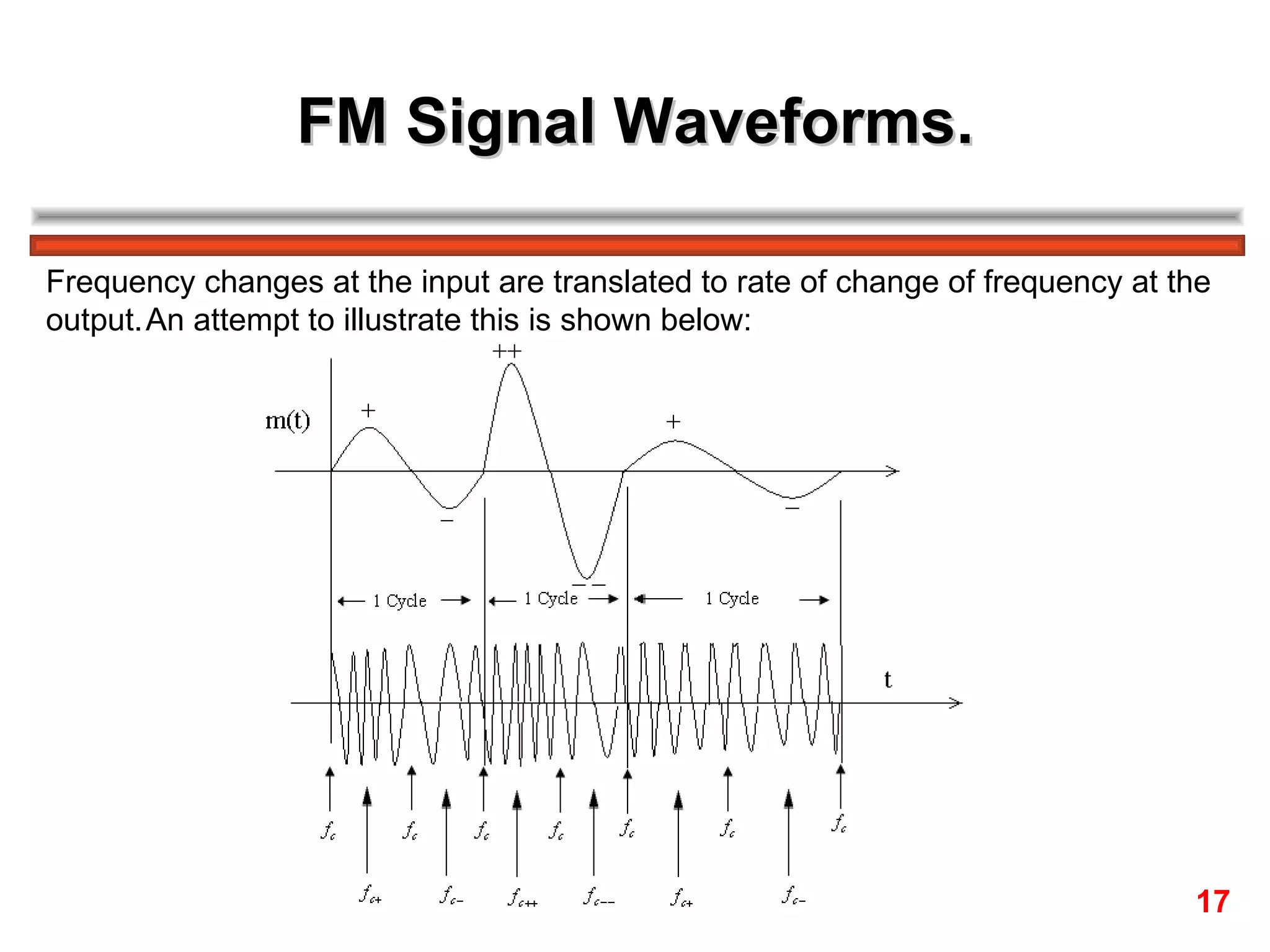
Frequency modulation (FM) varies the frequency of the carrier signal based on the message signal. There are two main types:
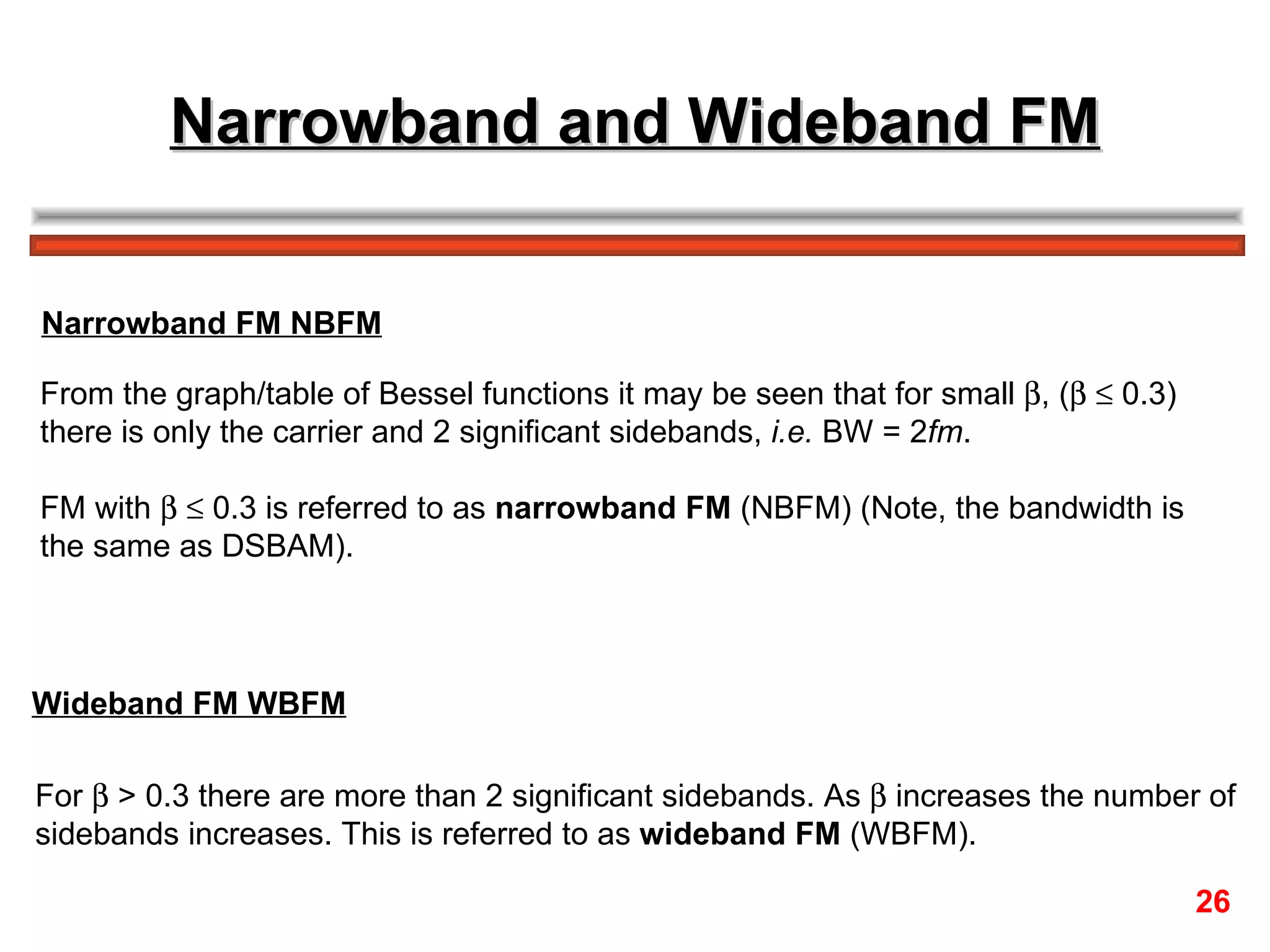
1. Narrowband FM varies the carrier frequency by a small amount (modulation index β ≤ 0.3), resulting in just the carrier and two significant sidebands.
2. Wideband FM uses a larger frequency deviation (β > 0.3), producing more than two sidebands.
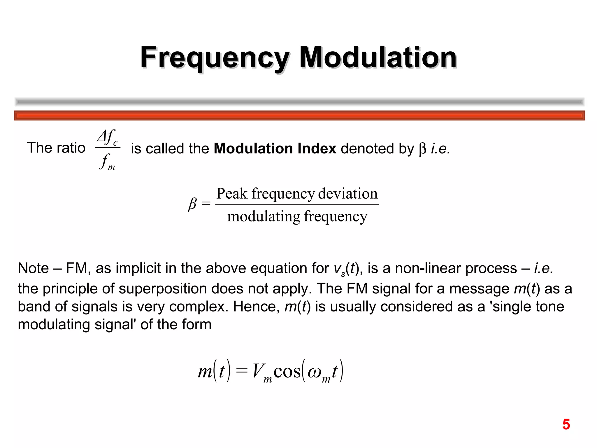
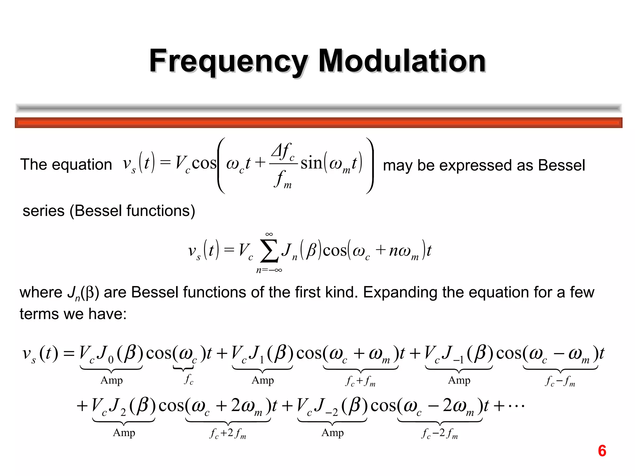
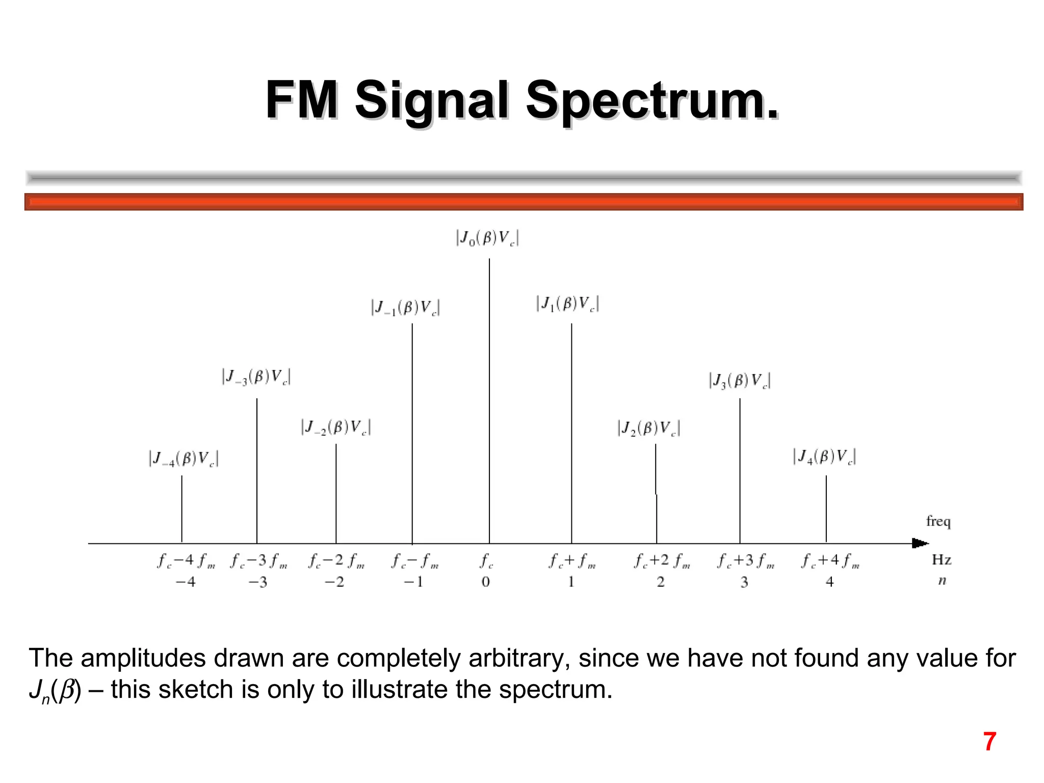
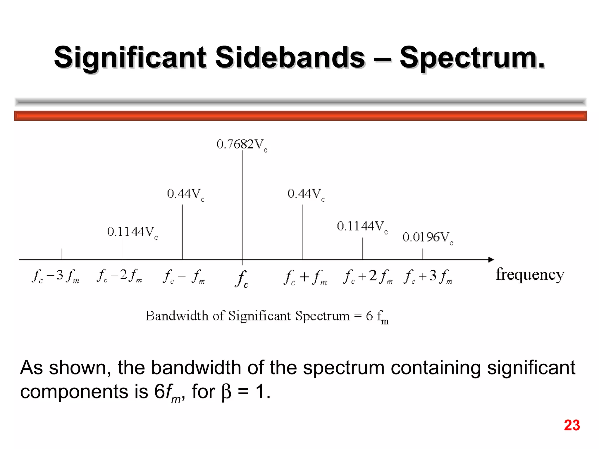
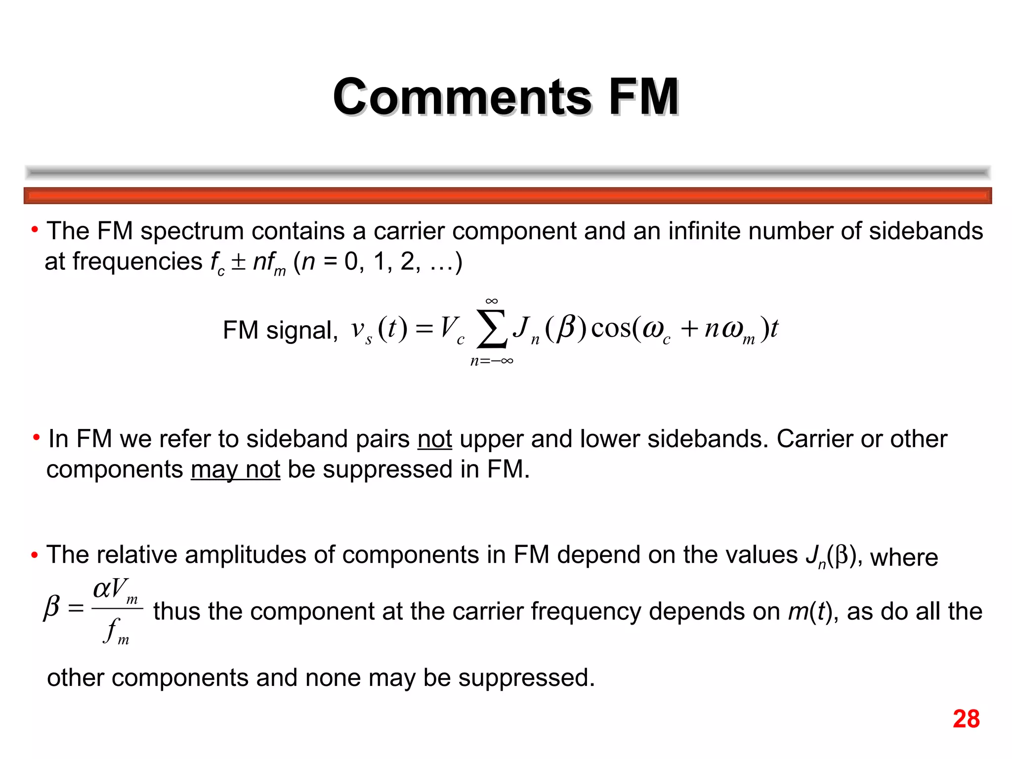
The FM spectrum consists of the carrier frequency fc and an infinite number of sideband frequencies at fc ± nfm, where the amplitudes are determined by Bessel functions and the modulation index β.