Gaussian model (kabani & sumeet)

GAUSSIAN MODEL
Sumeet Khirade
Kabani.K.S
M E Environmental Engineering (semester 1)
Sinhgad College of Engineering, Vadgaon, Pune
19/1/2015

INTRODUCTION
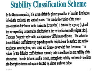
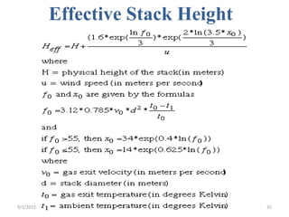
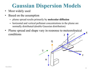
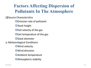
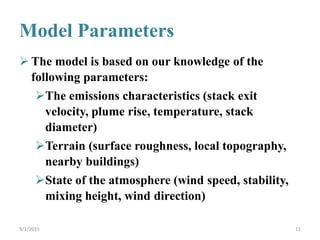
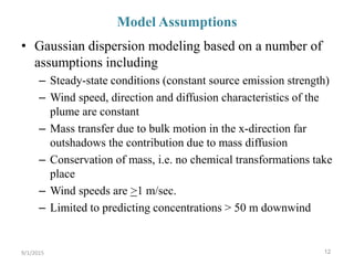
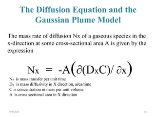
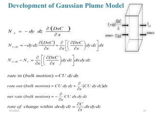
• The Gaussian plume model is a (relatively)
simple mathematical model that is typically
applied to point source emitters, such as coal-
burning electricity-producing plants to
determine the pollution.
• Occasionally, this model will be applied to
non-point source emitters, such as exhaust
from automobiles in an urban area.
29/1/2015

What is mathematical modeling?
When the process of problem reduction or
solution involves transforming some idealized
form of the real world situation into mathematical
terms,it goes under generic name of mathematical
modeling.
39/1/2015

Air Quality Modeling (AQM)
• Predict pollutant concentrations at various
locations around the source.
• Identify source contribution to air quality
problems.
• Access source impacts and design control
strategies.
• Predict future pollutant concentrations from
sources after implementation of new
regulatory programs.
49/1/2015

System approach to air quality model
What is air quality model ?
A mathematical relationship between emissions and air quality
that incorporates the transport, dispersion and transformation of
compounds emitted into the air.
59/1/2015

Air Quality Models
DETERMINISTIC STATISTICAL PHYSICAL
STEADY STATE TIME DEPENDENT
REGRESSION EMPIRICAL
WINDTUNNEL
SIMULATION
GAUSSIAN PLUME
BOX GRID PUFF TRAJECTORYSPECTRAL
LAGRANGIAN
EULERIAN
69/1/2015

The deterministic mathematical models calculate the
pollutant concentrations from emission inventory and
meteorological variables according to the solution of
various equations that represent the relevant physical
processes.
Deterministic modeling is the traditional approach for
the prediction of air pollutant concentrations in urban
areas.
What is deterministic approach?
79/1/2015

8
Gaussian Dispersion Models
• Most widely used
• Based on the assumption
– plume spread results primarily by molecular diffusion
– horizontal and vertical pollutant concentrations in the plume are
normally distributed (double Gaussian distribution)
• Plume spread and shape vary in response to meteorological
conditions
H
X
Y
Z
u
Q
9/1/2015

Factors Affecting Dispersion of
Pollutants In The Atmosphere
Source Characteristics
Emission rate of pollutant
Stack height
Exit velocity of the gas
Exit temperature of the gas
Stack diameter
 Meteorological Conditions
Wind velocity
Wind direction
Ambient temperature
Atmospheric stability
9/1/2015 10

Model Parameters
 The model is based on our knowledge of the
following parameters:
The emissions characteristics (stack exit
velocity, plume rise, temperature, stack
diameter)
Terrain (surface roughness, local topography,
nearby buildings)
State of the atmosphere (wind speed, stability,
mixing height, wind direction)
9/1/2015 11

12
Model Assumptions
• Gaussian dispersion modeling based on a number of
assumptions including
– Steady-state conditions (constant source emission strength)
– Wind speed, direction and diffusion characteristics of the
plume are constant
– Mass transfer due to bulk motion in the x-direction far
outshadows the contribution due to mass diffusion
– Conservation of mass, i.e. no chemical transformations take
place
– Wind speeds are >1 m/sec.
– Limited to predicting concentrations > 50 m downwind
9/1/2015

The Diffusion Equation and the
Gaussian Plume Model
13
The mass rate of diffusion Nx of a gaseous species in the
x-direction at some cross-sectional area A is given by the
expression
Nx = -A(∂(DxC)/ ∂x)Nx is mass transfer per unit time
Dx is mass diffusivity in X direction, area/time
C is concentration in mass per unit volume
A is cross sectional area in X direction
9/1/2015

Development of Gaussian Plume Model
149/1/2015

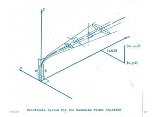
15
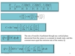
Where; x = along- wind coordinate measured in wind direction from the source
y = cross-wind coordinate direction
z = vertical coordinate measured from the ground
C(x,y,z) = mean concentration of diffusing substance at a point (x,y,z) [kg/m3]
Dy,Dz = mass diffusivity in the direction of the y- and z- axes [m2/s]
U = mean wind velocity along the x-axis [m/s]
Time rate of change and advection of the cloud by the mean wind
Turbulent diffusion of material relative to the center of the pollutant
cloud.( the cloud will expand over time due to these terms.)
9/1/2015

16
The rate of transfer of pollutant through any vertical plane
downwind from the source is a constant in steady state, and this
constant must equal the emission rate of the source, Q.
9/1/2015

17
Where Q is the strength of the emission source, mass
emitted per unit time
After integrating,
Gaussian parameters
9/1/2015

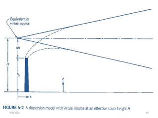
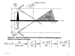
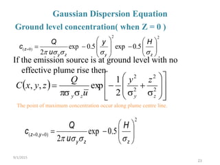
18
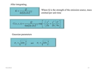
Where;
c( x, y, z ) = mean concentration of diffusing substance at a point ( x, y, z ) [kg/m3]
x = downwind distance [m],
y = crosswind distance [m],
z = vertical distance above ground [m],
Q = contaminant emission rate [mass/s],
σx = lateral dispersion coefficient function [m],
σy = vertical dispersion coefficient function [m],
U = mean wind velocity in downwind direction [m/s],
H = effective stack height [m].
9/1/2015

2-D STEADY DISPERSION MODEL
GROUND REFLECTION
• From the release height of H above ground,
dispersion can progress upward towards the mixing
height. In the downward direction the ground acts as
a mirror unless the pollutant gets deposited.
• The effect of the ground can be handled
mathematically by treating the reflection as another
point source located below ground (at - H)
9/1/2015 21

22
     




































 2
2
2
2
2
2
2
exp
2
exp
2
exp
2
,,
zzyzy
HzHzy
u
Q
zyxC
9/1/2015

23
Gaussian Dispersion Equation
If the emission source is at ground level with no
effective plume rise then
 





















 2
2
2
2
2
1
exp,,
zyzy
zy
u
Q
zyxC
Ground level concentration( when Z = 0 )
The point of maximum concentration occur along plume centre line.
9/1/2015
2
)0,0( 5.0exp
2 






zzy
yz
H
u
Q
c

22
)0( 5.0exp5.0exp
2 















zyzy
z
Hy
u
Q
c


31
CARAVAY’S METHOD
9/1/2015

34
Plume Rise
stackactualriseplume hhH 
9/1/2015

Effective Stack Height
359/1/2015

Advantages of Gaussian model
Produce results that match closely with experimental data
Simple in their mathematics
Quicker than numerical models
Do not require super computers
Disadvantages of Gaussian model
 Not suitable if the pollutant is reactive in nature
 Unable to predict concentrations beyond radius of approximately
20 Km
 For greater distances, wind variations, mixing depths and
temporal variations become predominant
399/1/2015

Conclusion
• Air pollution in cities is a serious public health
problem. Therefore, there is need for reliable
air quality management system for abatement
of urban air pollution problem
• Gaussian plume model is a very effective
method in determining pollutant
concentrations in atmosphere.
• Gaussian model is the most widely used AQM
to predict pollutant concentrations.
409/1/2015

REFERENCES
• Weber, E., “Air pollution assessment modeling methodology”, NATO,
challenges of modern society, vol.2, Plenum press, 1982
• Chastain, J.P. 1999. Air Quality and Odor Control from Swine Production
Facilities. chapter 9 in Confined Animal Manure Managers Certification
Program Manual, Clemson University, Clemson SC, pp 9-1 to 9-11,
http//hubcap.clemson.edu/scafrs/Peedee/certifi/CAMM.html.
• www.mfe.govt
• http://www.csiir.ornl.gov
• Rao, M.N. and Rao, H. V. N., 1993. Air Pollution, Tata Mc-Graw Hill, New
Delhi.
• Murty, B. P., 2004. Environmental Meteorology, I.K. International Pvt.
Ltd., New Delhi.
419/1/2015

Gaussian model (kabani & sumeet)

More Related Content

What's hot

Viewers also liked

Similar to Gaussian model (kabani & sumeet)

Recently uploaded

Gaussian model (kabani & sumeet)