Downloaded 107 times


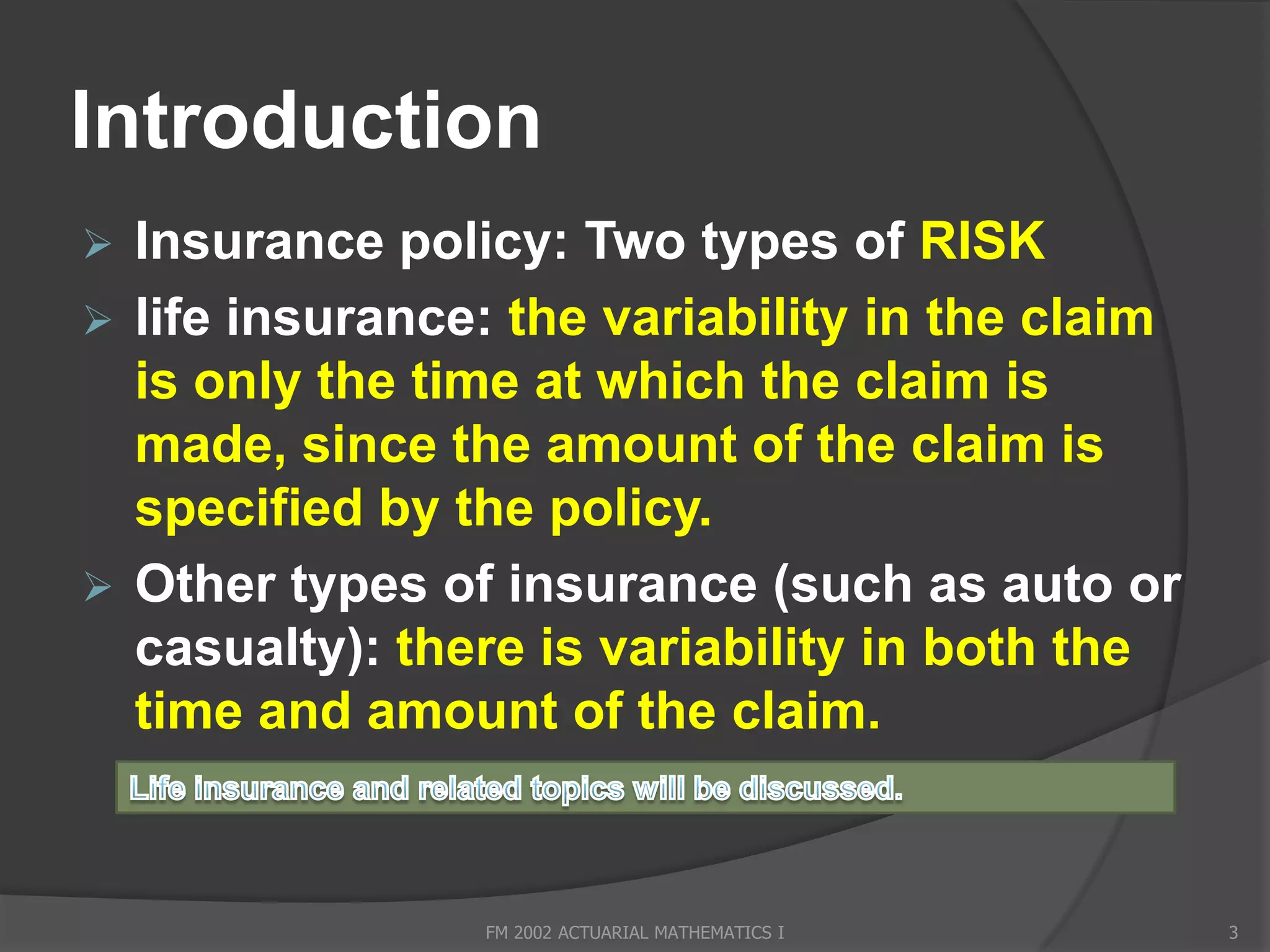
![Survival Function
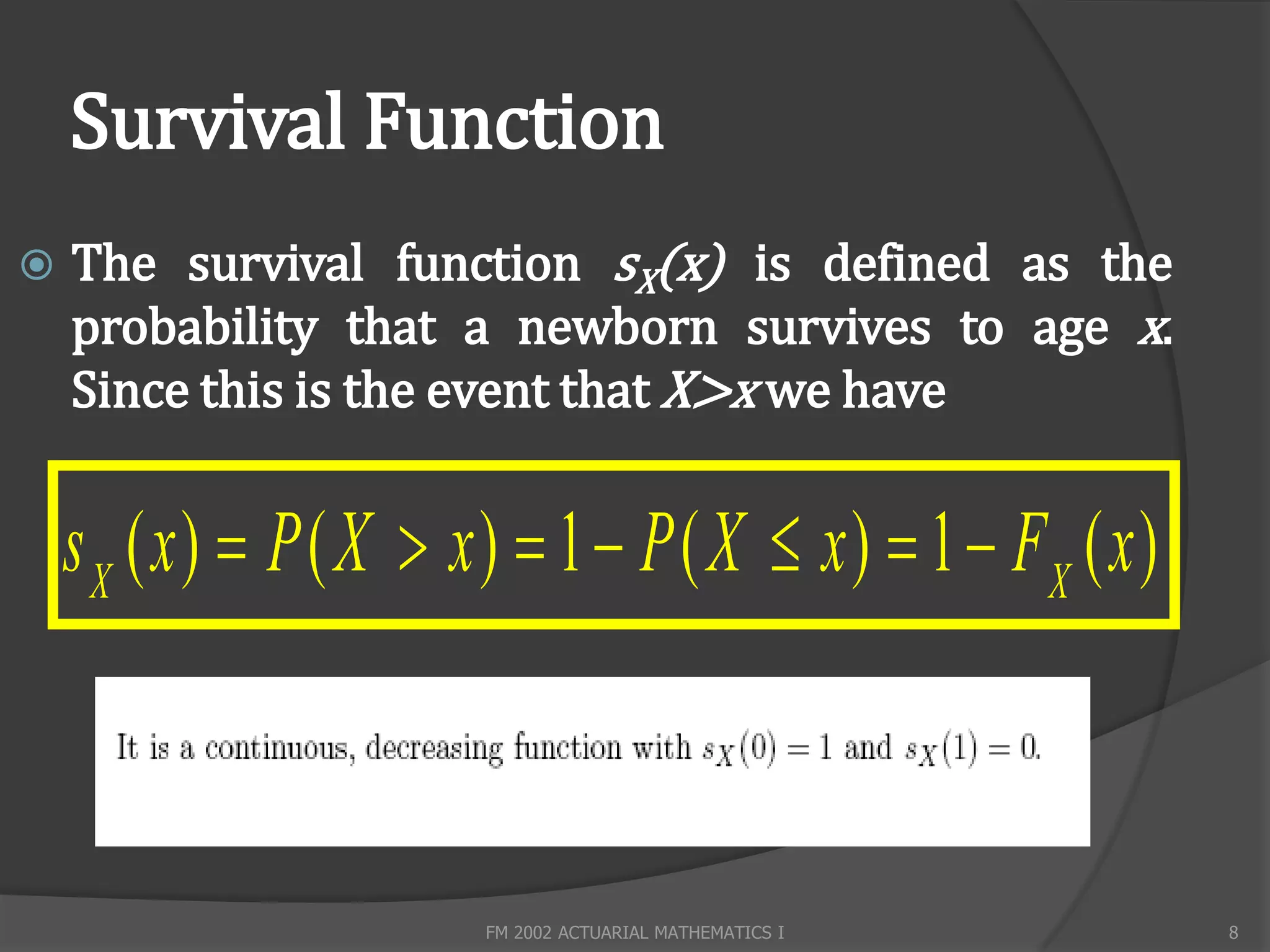
The basic of a survival model is a
random lifetime variable and its
corresponding distribution.
X: Life time of a newborn.
X: Cts, X [0, ]
f X ( x)
Probability density function
Probability distribution F ( x )
X
FM 2002 ACTUARIAL MATHEMATICS I 6](https://image.slidesharecdn.com/lecture1-130103010151-phpapp01/75/Acturial-maths-6-2048.jpg)

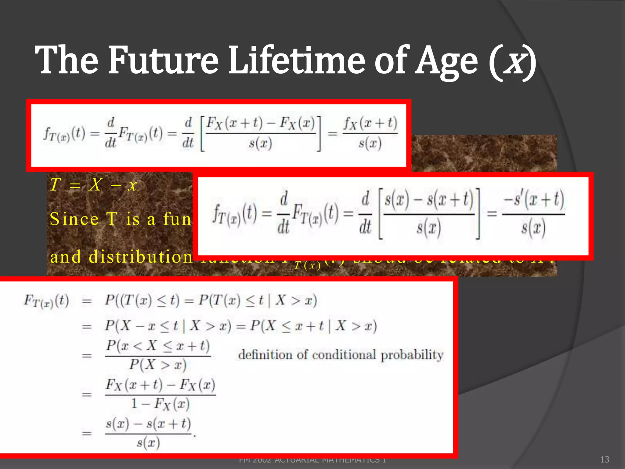
![The Future Lifetime of Age (x)
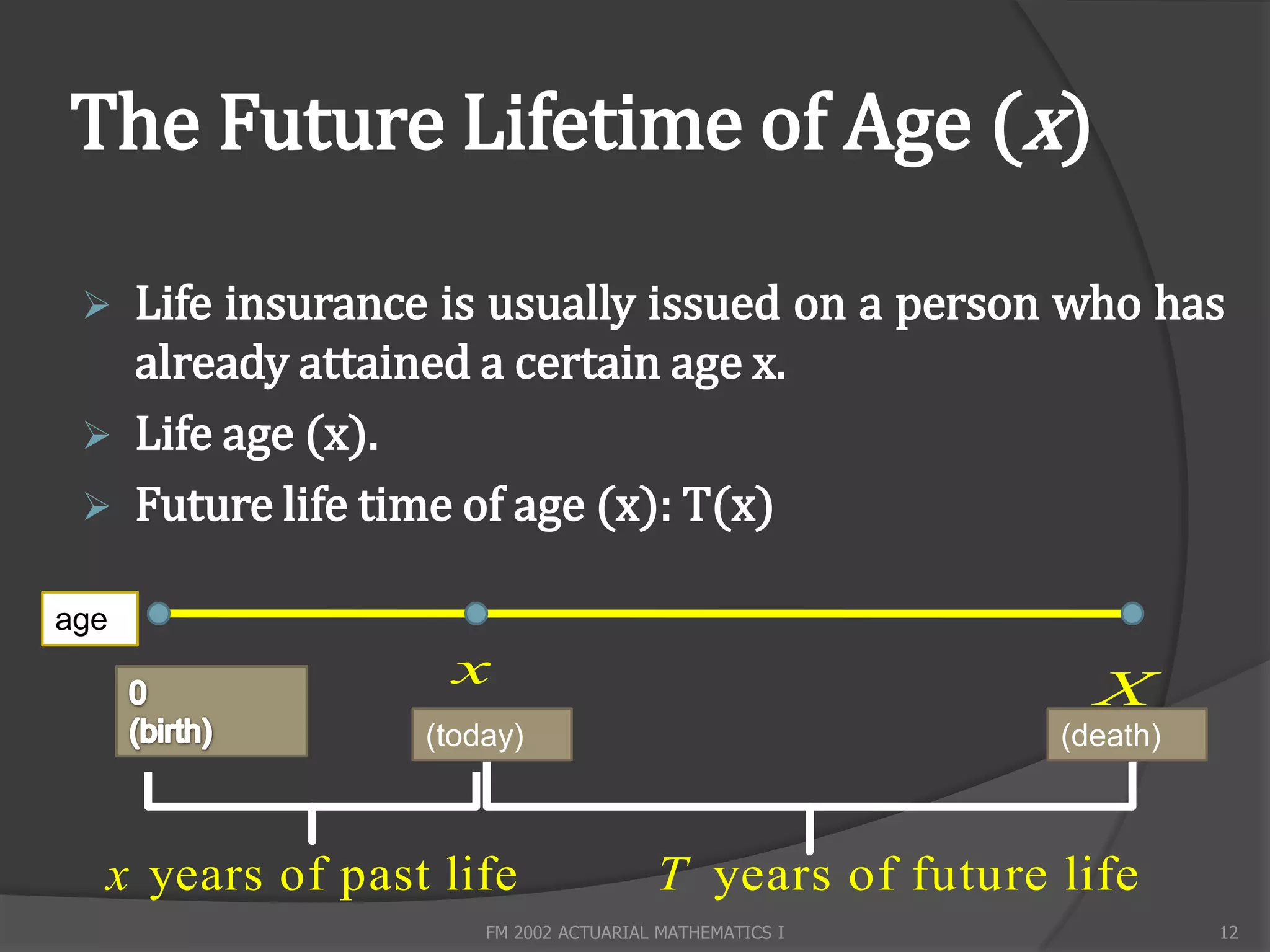
This gives the conditional probability that a newborn will die
between the ages x and x+t. OR
age (x) dies before reaching to age x+t, OR
age (x) dies within next t years.
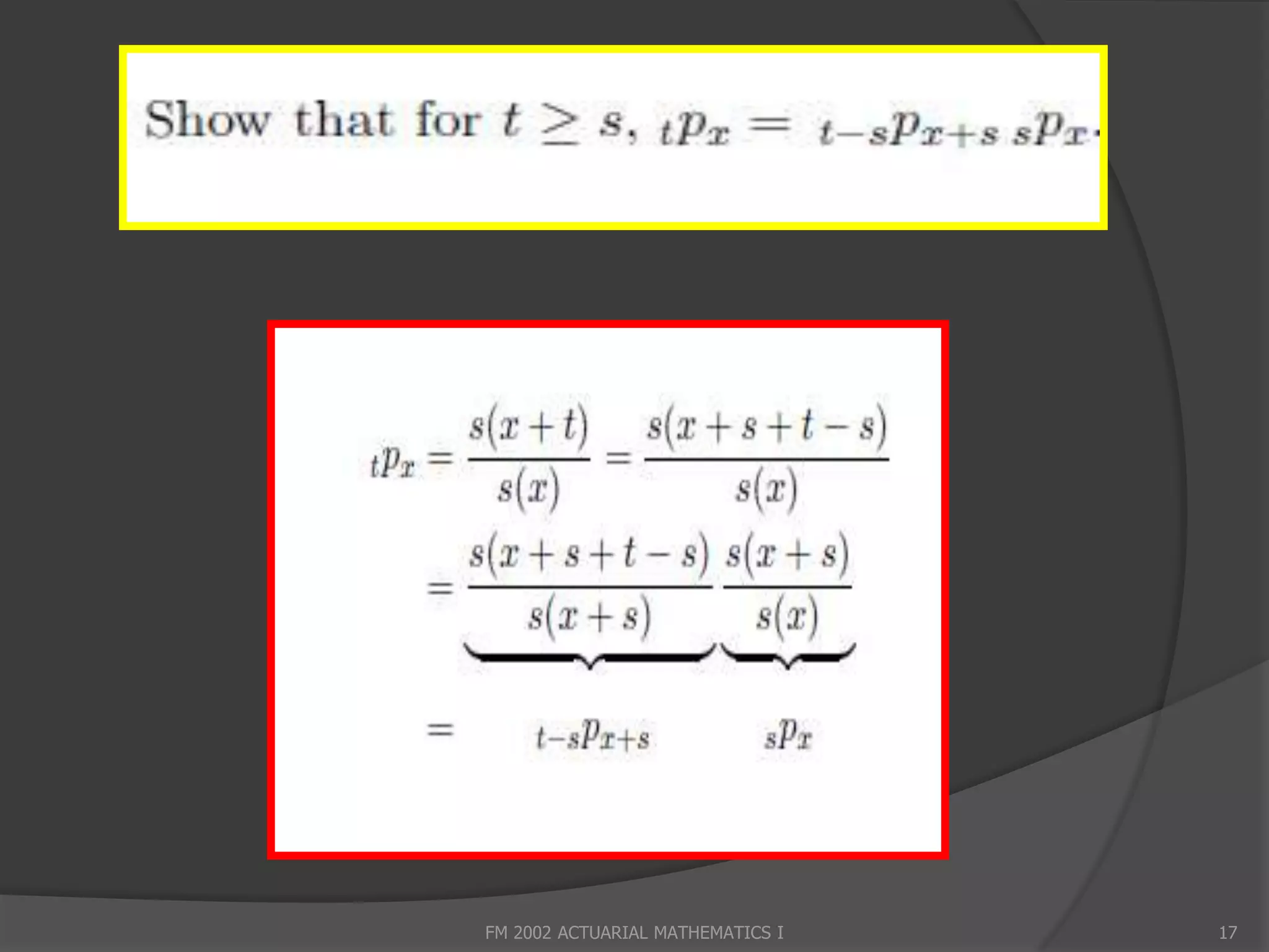
t
p x the probability of survival to age x t give n survival to age x.
= P[T ( x ) t ]
t
q x the probability of death before age x t giv en survival to age x.
= P[T ( x ) t ] 1 t p x
FM 2002 ACTUARIAL MATHEMATICS I 14](https://image.slidesharecdn.com/lecture1-130103010151-phpapp01/75/Acturial-maths-14-2048.jpg)
![Remarks
T he sym bol, t q x can be interpreted as the p robability that ( x ) w ill die w ithin t years;
that is t q x is the distribution function of T ( x ).
T he sym bol, t p x can be interpreted as the p robability that ( x) w ill survive another t years;
that is t p x is the survival function of T ( x).
W hen t 1 the prefix is om itted and one j ust w rites p x and q x respectively.
p x = P [T ( x ) 1], the probability that ( x) survive s another year.
q x P [T ( x ) 1], the probability that ( x) w ill die w ithin next ye ar.
FM 2002 ACTUARIAL MATHEMATICS I 15](https://image.slidesharecdn.com/lecture1-130103010151-phpapp01/75/Acturial-maths-15-2048.jpg)

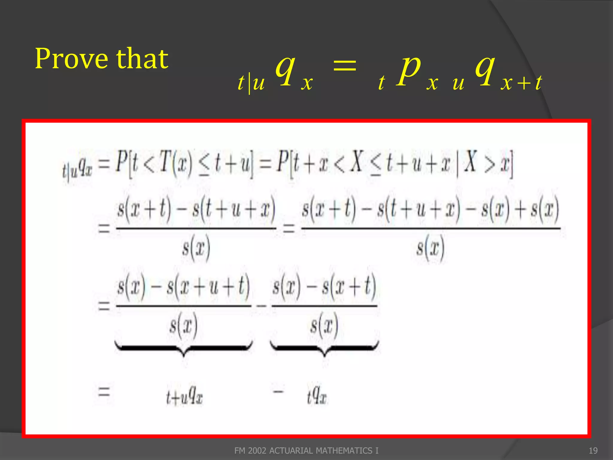
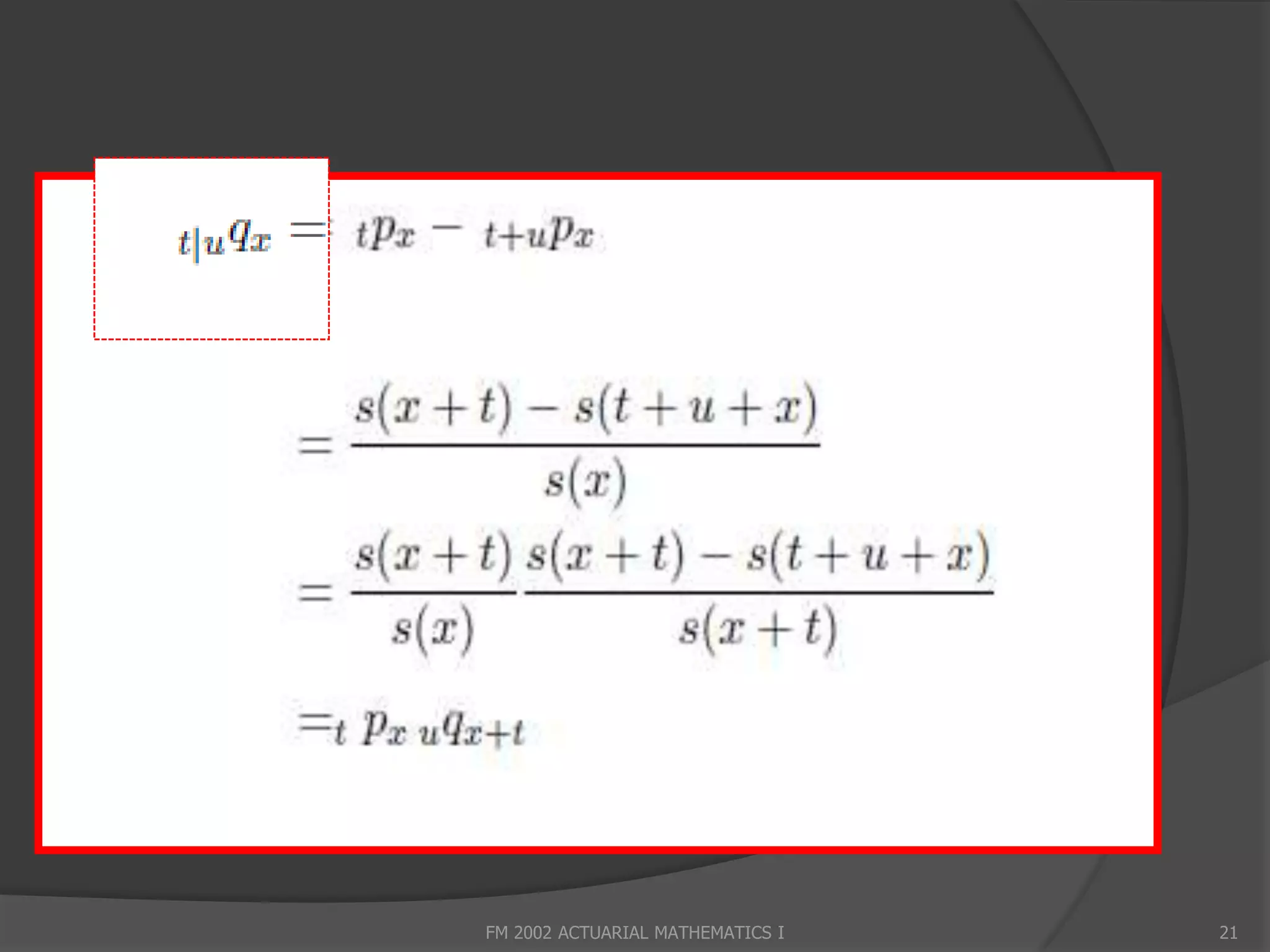
![Special symbol
(x) will survive t years and die within the
following u years: i.e. (x) will die between ages
x+t and x+t+u.
t |u
q x P [t T ( x ) t u ] P [ x t X x t u ]
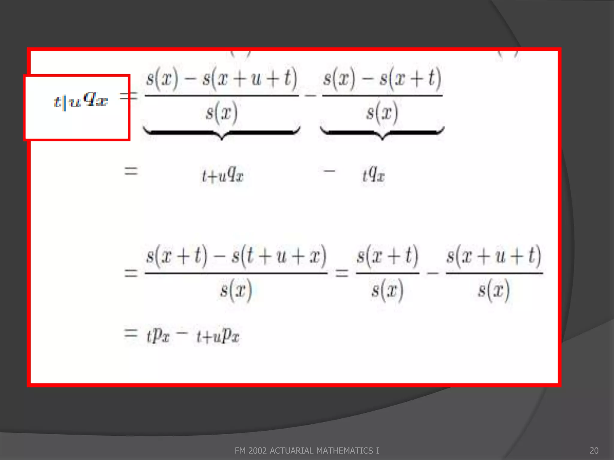
t |u
qx t u
qx t qx t
px t u
px
t |u
qx t
px u
q x t
FM 2002 ACTUARIAL MATHEMATICS I 18](https://image.slidesharecdn.com/lecture1-130103010151-phpapp01/75/Acturial-maths-18-2048.jpg)
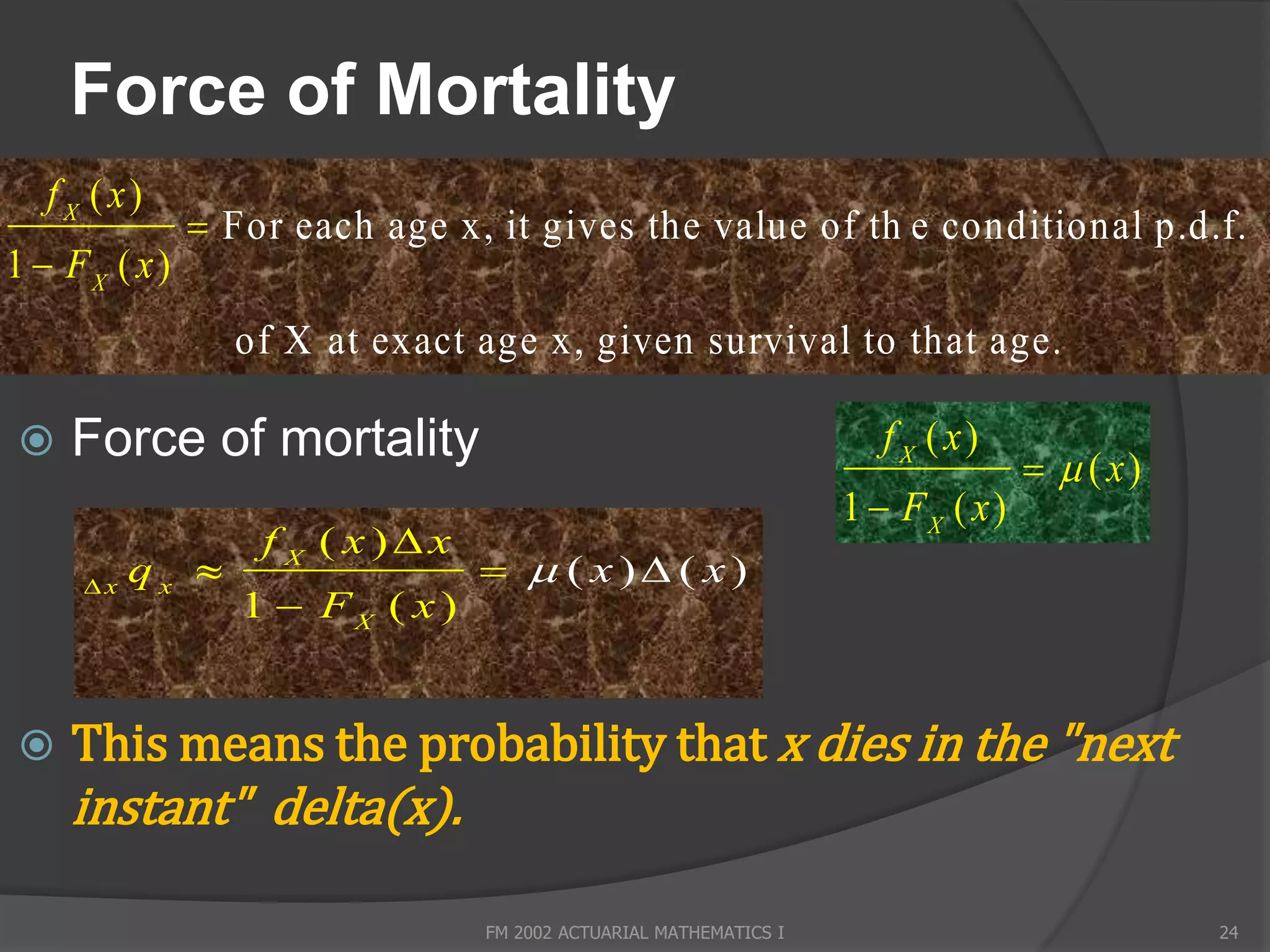
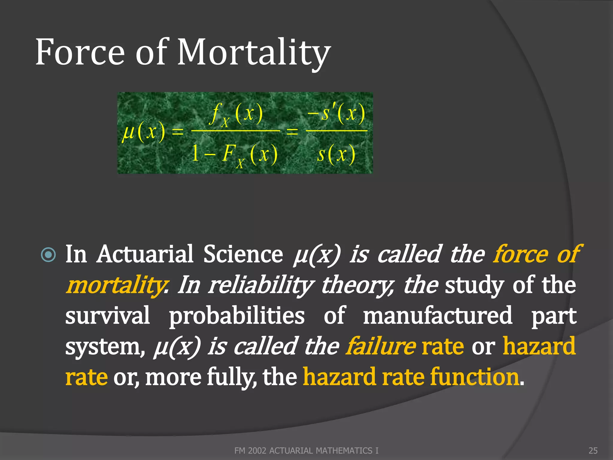
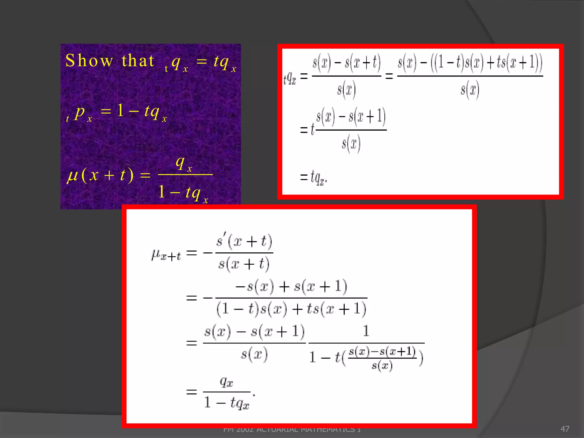
![Force of Mortality
Consider s( x) s( x t)
t
q x P[ x X x t | X x ]
s(x)
Now take t=Δx
FX ( x x ) FX ( x )
x
q x P[ x X x x | X x ]
1 FX ( x )
FX ( x x ) FX ( x ) x f X ( x)x
=
x 1 FX ( x ) 1 FX ( x )
FM 2002 ACTUARIAL MATHEMATICS I 23](https://image.slidesharecdn.com/lecture1-130103010151-phpapp01/75/Acturial-maths-23-2048.jpg)
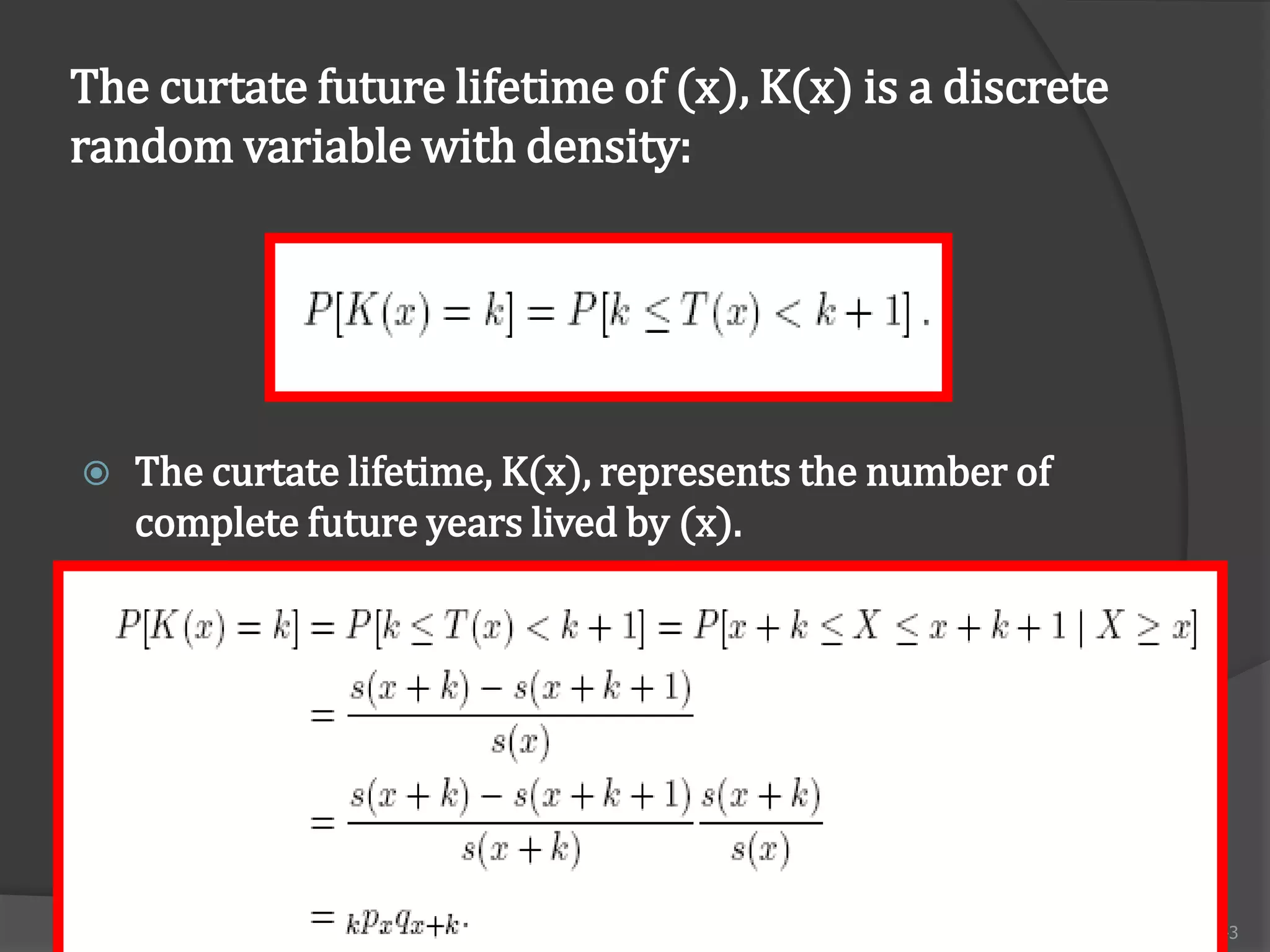
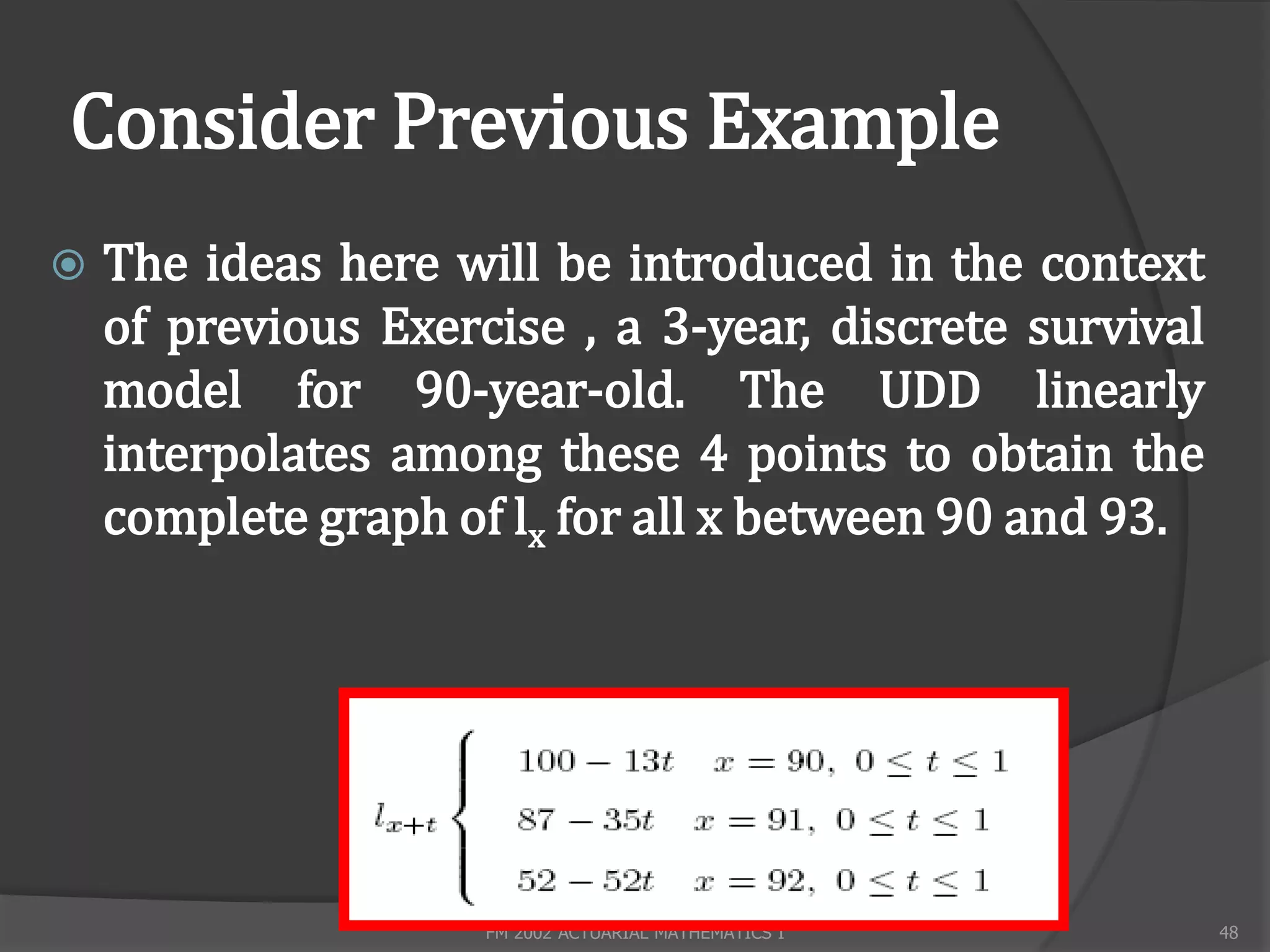
![Curtate Future Lifetime
A discrete random variable associated with the
future lifetime is the number of future years
completed by (x) prior to death. It is called the
curtate future lifetime of (x), denoted by K(x), is
defined by the relation:
K ( x ) T ( x )
Here [ ] denote the greatest integer function.
FM 2002 ACTUARIAL MATHEMATICS I 42](https://image.slidesharecdn.com/lecture1-130103010151-phpapp01/75/Acturial-maths-42-2048.jpg)
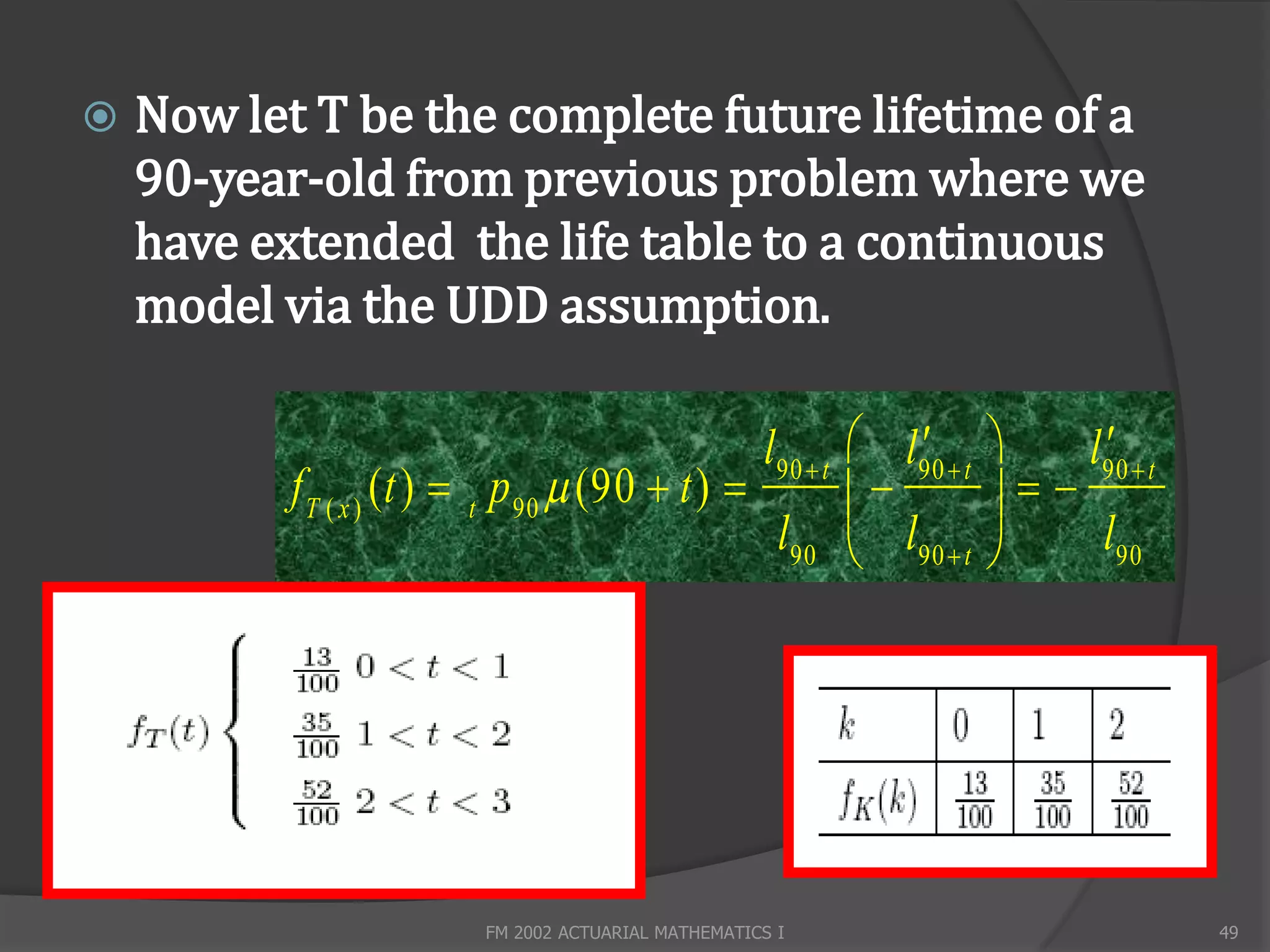
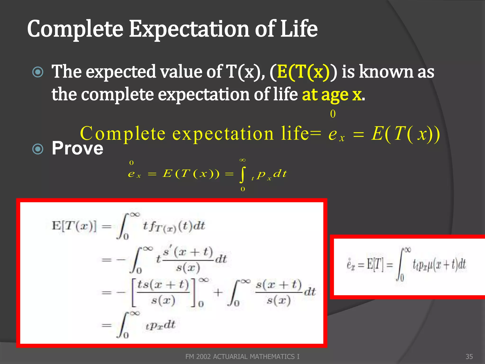
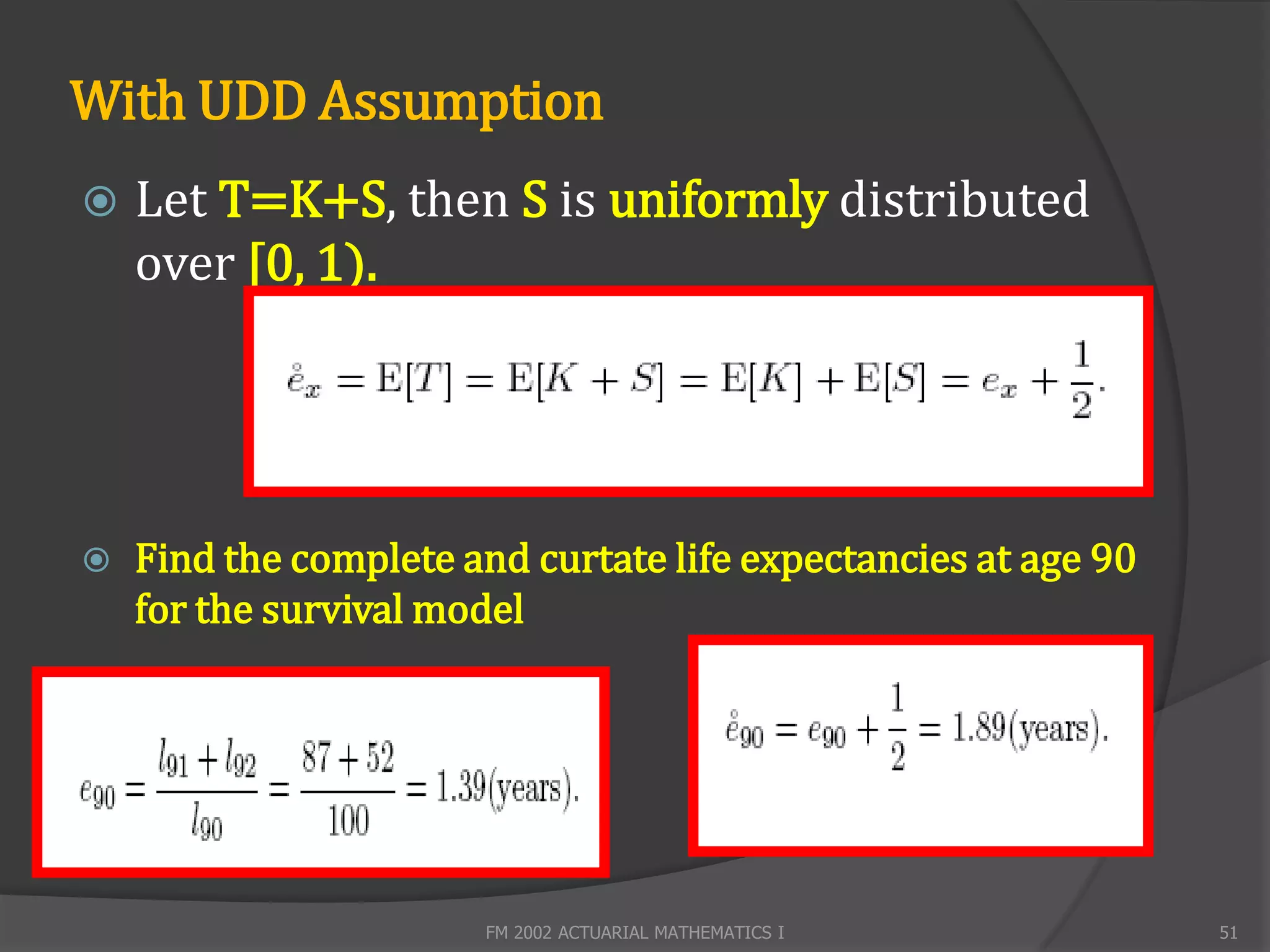
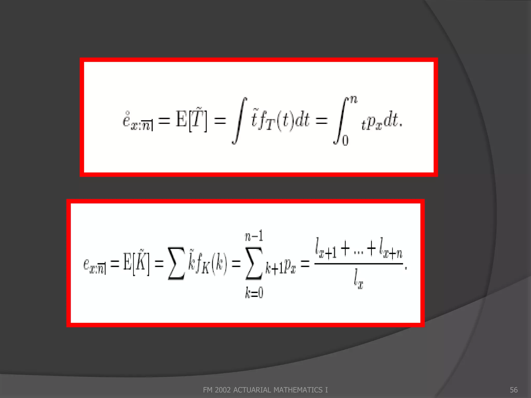
![Curtate Life Expectancy
E(K) is known as the complete life expectancy and is
denoted by ex
x 1 x 1
ex E [ K ] kf K ( x ) ( k ) k k pxqxk
k 0 k 0
x
0 x x
lxt
lxt dt
ex p x dt dt 0
t
0 0
lx lx
x 1 x 1
l x k 1 l x 1 l x 2 ... l 1
ex k 1
px lx
lx
k 0 k 0
FM 2002 ACTUARIAL MATHEMATICS I 50](https://image.slidesharecdn.com/lecture1-130103010151-phpapp01/75/Acturial-maths-50-2048.jpg)
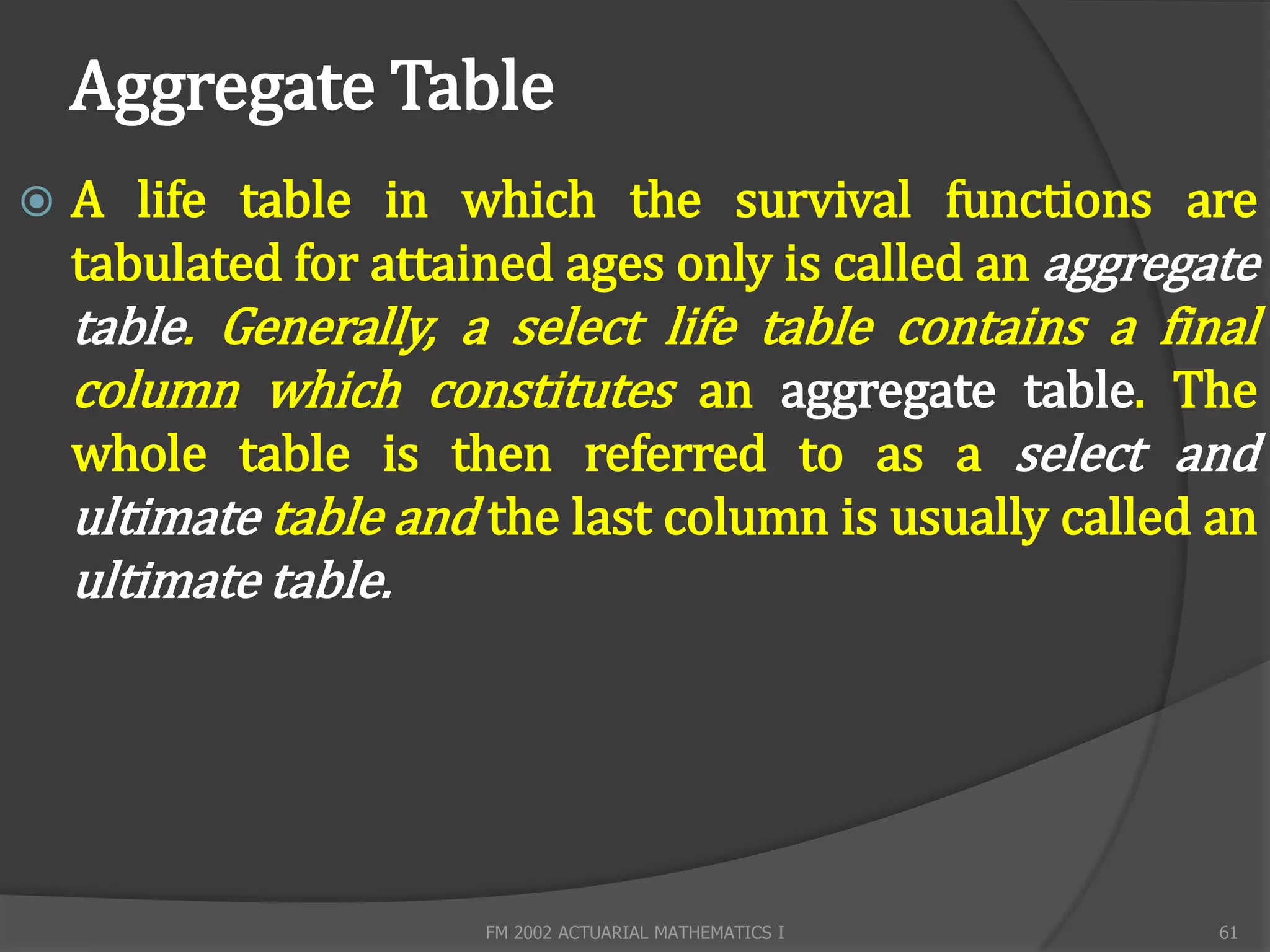
![Notations
q[x]+i denotes the probability that a person dies between years x +
i and x + i + 1 given that selection occurred at age x.
q25 - Probability that an insured 25-old will die in the
next year.
q25 values for individuals underwritten at ages 0, 1, 2,
...,24, 25 are respectively denoted by q[0]+25, q[1]+24, …, q[25].
FM 2002 ACTUARIAL MATHEMATICS I 59](https://image.slidesharecdn.com/lecture1-130103010151-phpapp01/75/Acturial-maths-59-2048.jpg)
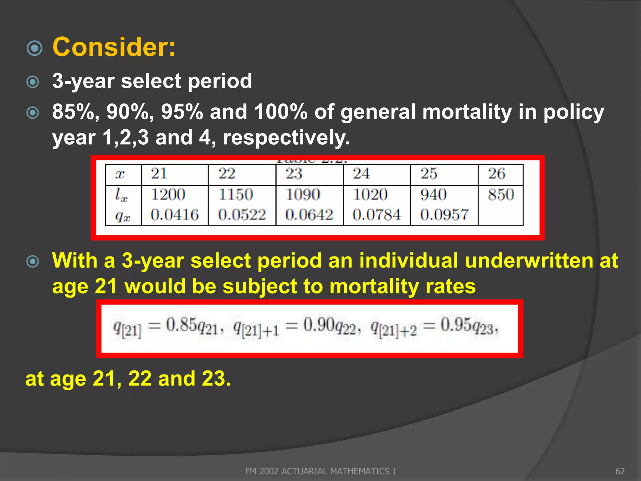
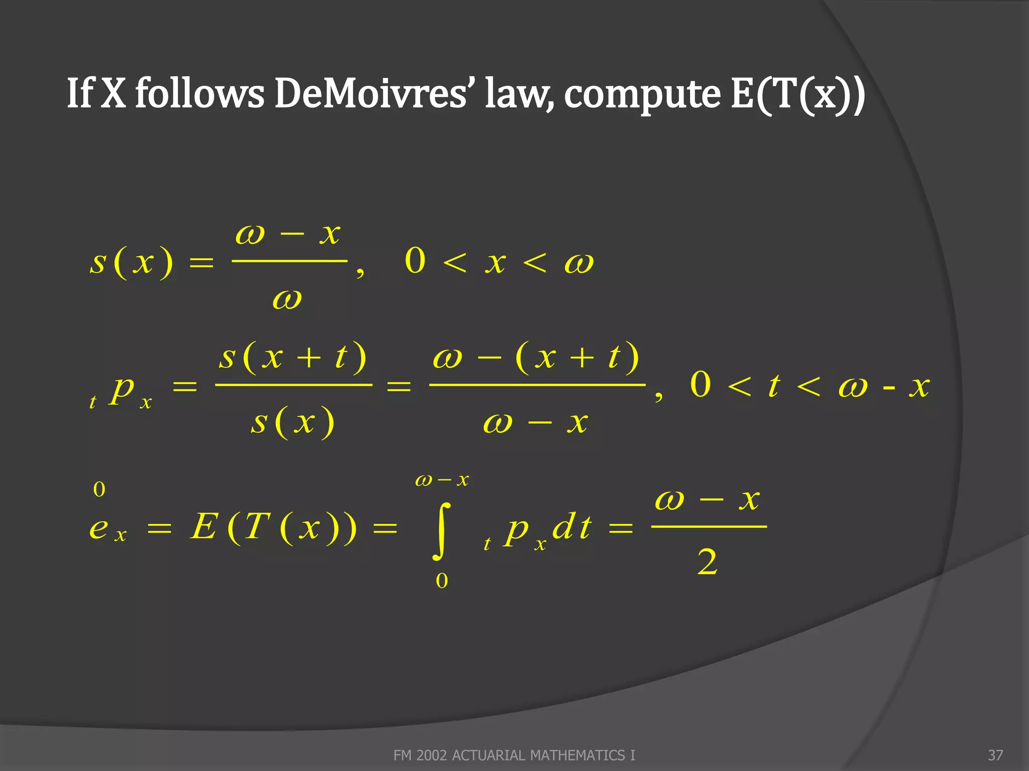
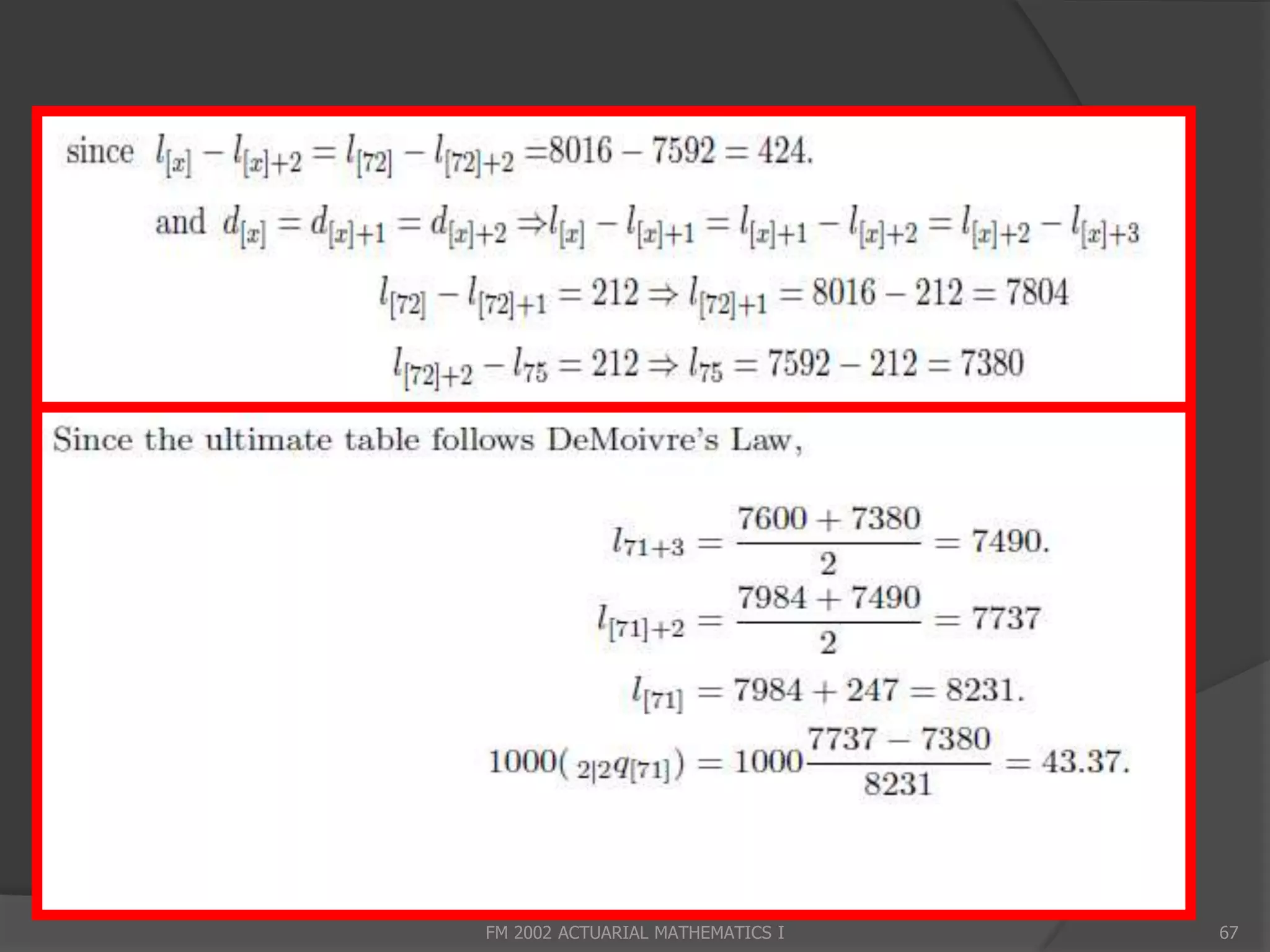
![ You are given the following extract from a 3
year select and ultimate mortality table.
Assume that the ultimate table follows
DeMoivre’s law and that d[x]=d[x]+1=d[x]+2 for
all x. Find 1000( 2|2q[71] )
FM 2002 ACTUARIAL MATHEMATICS I 65](https://image.slidesharecdn.com/lecture1-130103010151-phpapp01/75/Acturial-maths-65-2048.jpg)
![2|2
q [ 71] P robability of age 71 survies tw o years and
w ill die the follow ing 2 years.
FM 2002 ACTUARIAL MATHEMATICS I 66](https://image.slidesharecdn.com/lecture1-130103010151-phpapp01/75/Acturial-maths-66-2048.jpg)

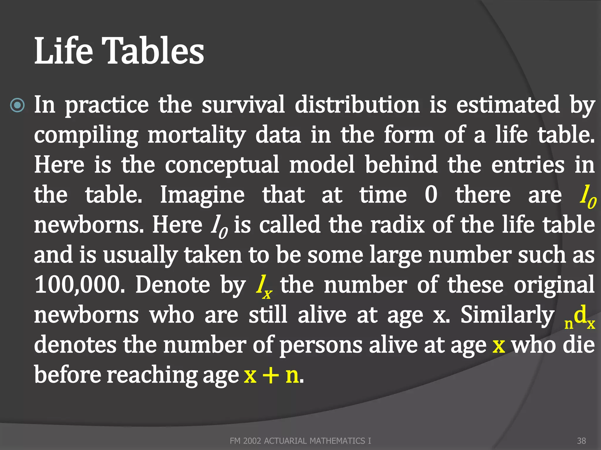
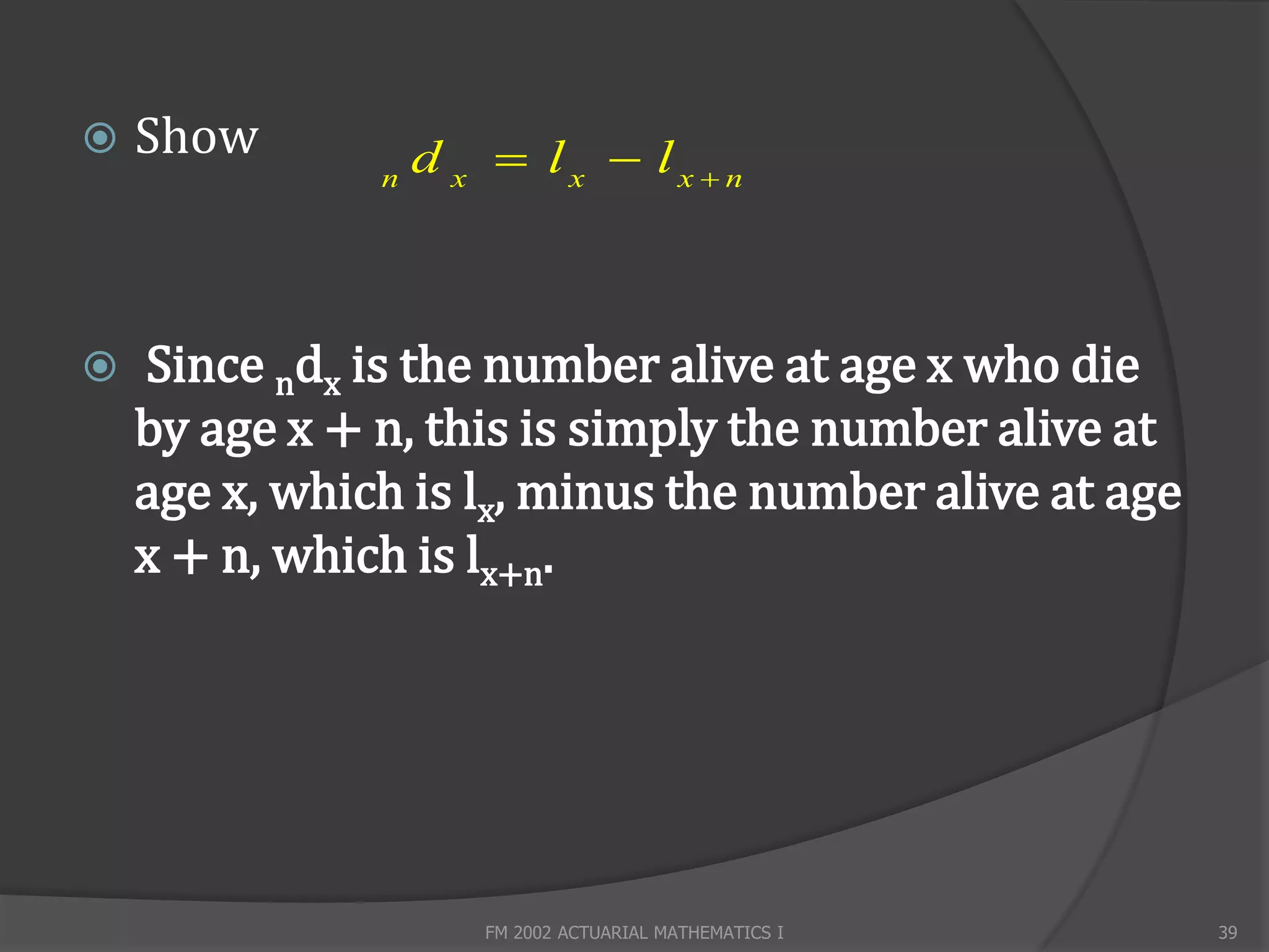
Here are the key entries in a life table and how they relate: - l0 is the initial number of lives (radix) - lx is the number of lives alive at age x - dx is the number of deaths between age x and x+1 - qx is the probability of dying between age x and x+1 (called the central death rate) We can write: dx = lx - lx+1 qx = dx / lx So dx represents the number of deaths between age x and x+1. It is calculated as the difference between the number of lives alive at the start of the interval (lx) and the number alive at the end (lx+1).


![[Actuary] actuarial mathematics and life table statistics](https://cdn.slidesharecdn.com/ss_thumbnails/actuaryactuarialmathematicsandlife-tablestatistics-120627131254-phpapp01-thumbnail.jpg?width=640&height=640&fit=bounds)


