This document provides an overview of key concepts related to quadratic expressions and equations. It discusses: 1) How to identify and form quadratic expressions, including factorizing expressions of various forms. 2) How to write and solve quadratic equations using methods like factoring and the quadratic formula. 3) Key terms like roots, intercepts, and the relationship between the gradient of a line and its steepness and direction.

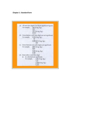
1. Chapter 1 : Standard form

2. Chapter 2 : Quadratic expressions and Equations
2.1 Quadratic expressions
* Identifying quadratic expressions
1. A quadratic expression in the form ax2
+bx+c,where a,b and c are constants,a≠0 and × is an unknown.
For example:
(a) 3x2 - 4x + 5
(b) 2x2 + 6x
(c) x2-9
2.In a quadratic expression:
 there is only one unknown
 the highest power of the unknown is 2
* Forming quadratic expressions by multiplying two linear expressions
1. When two linear expressions with the same unknown are multiplied,the product is a quadratic
expression.
2. The multiplication process is known as expansion
* Forming quadratic expressions based on specific situations
To form quadratic expressions based on specific situations :
1.Choose a letter to represent the unknown.2.Form a quadratic expressions based on the information
given.
2.2 Factorisation of quadratic expressions
*Factorising quadratic expressions of the form ax2
+ bx + c,where b =0 or c =0
1.When b = 0, ax2
+ c can be factorised by finding the highest common factor (HCF) of the coefficients a
and c.

3. 2.When c=0,ax2
x< + bx can be factorised by finding the highest common factor of the
coefficients a and b.x is also a common factor of the two terms.
*Factorising quadratic expressions of the form px2
- q,where p and q are perfect squares
Let p = a² and q = b²
px² - q = (ax)² - b²
= (ax + b) (ax - b)
*Factorising quadratic expressions of the form ax2
+ bx + c, where a ≠ 0, b ≠ 0 and c ≠ 0
1.We can use the inspection method and cross method to factorise quadratic equations of this form.
2.To factorise quadratic expressions :
(a) ax² + bx + c, where a = 1
x² + bx + c =(x + p) (x + p)
=x² + qx + px + q²
=x² + (p + q) x + pq
In comparison,
b = p + q ,c = pq
- Find the combination of two numbers whose product is c.
- Choose the number combination from step 1 whose sum is b.
(b) ax² + bx + c, where a > 1
ax² + bx + c =(mx + p) (nx + q)
=mnx² + mqx + npx + pq
=mnx² + (mq + np) x + pq
In comparison,
a = mn , b = mq + np , c = pq
- Find the combination of two numbers whose product is a.

4. - Find the combination of two numbers whose product is c.
- Choose the number combination from step 1 and step 2 whose sum is b.
*Factorising quadratic expressions containing coefficients with common factors
For quadratic expressions containing coefficients with common factor first before
carrying out the factorisation of the expressions.
2.3 Quadratic Equations
* Indentifying quadratic equations with one unknown
1. Quadratic equations with one unknown are equations involving quadratic expressions.
2. In a quadratic equation :
 there is an equal sign '='
 there is only one unknown
 the highest power of the unknown is 2
* Writing quadratic equadratic equations in general form
The general form of quadratic equations is ax2
+ bx + c = 0,
where a,b and c are constants,a ≠ 0 and x is an unknown.
* Forming quadratic equations based on specific situations
To form quadratic equation based on specific situations :
1.Choose a letter to represent the unknown.
2.Form a quadratic equation based on the information given.
2.4 Roots of Quadratic Equations
* Determining the roots of a specific quadratic equation
The roots of a quadratic equation are the values of the unknown which satisfy the quadratic equation.

5. * Determining the solutions for quadratic equations
1.The solutions for a quadratic equation can be determined by :
 Trial and improvement method
 Factorisation
2.To determine the solutions for ax2
+ bx + c = 0 using trial and improvement method :
 Try using the factors of the last term,c.
 If a > 1, try using fractions with a as the denominator and the factors of c as numerator.
3.To determine the solutions for ax² + bx + c = 0, using factorisation method :
 Factorisation the equation to the from (mx + p)(nx + q) = 0
 Equate each factor to zero to obtain the solutions.
mx + p = 0 nx + q = 0
x = - p x = - q
m m
Chapter 3 Sets
3.1 Sets
* Sorting objects into groups
A set is a collection of objects with common characteristics.
* Defining sets
1. Sets are usually denoted by capital letters.
2. There are two ways to define a set :
 By descriptions
 By set notations, { }

6. *Identifying elements of a set
1.The objects in a set are known as elements.
2.For example,if A is a set of even numbers,then 2 is an element of set A.
We write 2 ∈ A an 5 ∉ A.
3.The symbol ∈ is used to denote the phrase 'is an element of' or' is a member of'.
*Representing sets using Venn diagrams
1.Sets can be represented using Venn diagrams.
2.A Venn diagram is an enclosed geometrical diagram in the shape of a circle,ellipse,triangle,square or
rectangle.
3.For example,A = {1,2,3,4} can be represented in the Venn diagram below.
4.Notice that there are 4 elements in set A.Set A can also be represented in a Venn diagram as
follows.
*Listing elements and stating the number of element in a set
We use the notation n(A) to represent the number of elements in set A.
*Empty sets
1.An empty set is a set with elements.
2.We use { } or to represent empty sets.
3.For example,M = {x : x < 0 and x is a positive integer} is an empty set as M contains no elements.We
write M = or M = { }
*Equal set
1.Two sets,A and B are equal if both have the same elements.

7. 2.For example,A = { 1,2,3,4} and B = {2,4,3,1} are equal sets.It is written as A = B.
3.If set M is not equal to set N,then it is denoted as M ≠ N
3.2 Subset,Universal Set and the Complement of a set
*Subsets
1.Element of set A is also an element of set B,then A is a subset of B.
2.if not all the elements of set M are the elements of set N,then M is not the subset of N.The
relationship is
written as M ¢ N
*Representing subsets using Venn diagrams
Subsets can be represented using Venn diagrams.
*Listing the subsets of a specific set
Given that A = {1,2,3}.The possible subsets of A are ,{1},{2},{3},{1,2},{1,3},{2,3} and {1,2,3}.
*Universal set
1.Universal set is a set consisting of all the elements under discussion.
2.the symbol is used to denote a universal set.
3.All the sets under discussion are subsets of the universal set.
*The complement of a set

8. 1.The complement of set A is a set consisting of all the elements in ,which are not the elements of set A
2.The symbol A' denotes the complement of set A.
3.In the Venn,diagram below,the shaded region represents A'
3.3 Operation on Sets
*Intersection of sets
1.Intersection of set A and B is a set of elements which common to both sets A and B.
2.The intersection of set A and B is denoted by A B.
3.The shaded region in Venn diagram represents A B.
*The complement of the intersection of sets
1.The complement of A ∩ B is a set containing all the elements which are not the elements of set A ∩ B.
This is denoted by (A ∩ B)'.
2.The shaded region in the Venn diagram below represents

9. (A ∩ B)'.
*Solving problems involving the intersection of sets
We can solve some problems in our daily life by applying the concepts of the intersection of sets.
*Union of sets
1.The union of sets A and B is a set of elements belonging to either of the sets or both.
2.The symbol A B denotes the union of set A and B.
*The complement of the union of sets
1.The complement of A U B is a set containing all the elements in the universal set, ξ which are not
elements
of the set A U B.This is denoted by (A U B)'.
2.The shaded region in Venn diagram represent (A U B)'.

10. *Solving problems involving the union of sets
Venn diagram is very useful when solving problems involving the union of sets.
*Combined operations on setsWhen combined operations are involved,carry,out the operations in the
brackets first.
*Solving problems involving combined operations on sets
Venn diagram is very useful when solving problems involving the union of sets
Chapter 4 Mathematical Reasoning
4.1 : Statements
*Determining whether a sentence is a statement
 A statement is a sentence that is either true or false but not both.
4.2 : Quantifiers "All" and "Some"
* Constructing statements using the quantifiers "all" and "some"

11. A quantifiers denotes the number of objects or cases involved in a statement.
(a) "All" refers to each and every object or case that satisfies a certain condition.
(b) "Some" refers to several and not every object or case that satisfies a certain condition.
*Determining the truth value of statements that contain the quantifier "all"
In statement that contains the quantifier "all",each and every objects is being considered in
the statement.If there is one object (or more) that contradicts the statement,then the statement is
false.
*Generalising statements using the quantifier "all"
Sometimes a statement can be generalised to cover all cases using the quantifier "all" without changing
its truth value.
*Constructing true statements using the quantifier "all" or "some"
To construct a true statement based on given objects and their properties :
(a)Use the quantifier "all" if each and every object satisfies the given property.
(b)Use the quantifier "some" if there is one or more objects that contradicts with the given property.
4.3 Operations on Statements
*Changing the truth value of statements using the word "not" or "no"
1.The word "not" or "no" can be used to change the truth value of a statement.
2.The process of changing the truth value of a statement using the word "not" or "no" is known as
negation.
3.~p represent the negation for statement p.
4.Example:
*Identifying two statement from a compound statement that contains the word "and"
1.In compound statement containing the word "and" we can identify two statement.

12. 2.For example,7 is an odd number and 14 is an even number.Is a compound statement that is made up
from the following two statement.
statement 1 : 7 is an odd number.
statement 2 : 14 is an even number.
*Forming compound statement using the word "and"
W can use the word "and" to from a compound statement from two statement.
*Identifying two statement from a compound statement that contains the word "or"
In a compound statement containing the word "or" we can identify two statement.
statement 1 : -5 < -2
statement 2 :½ = 0.5
*Forming compound statements using the word "or"
We can from compound statement from two statement by using the word "or"
*Truth value of compound statement that contains the word "and"
1.When two statements are combined with the word "and" the compound statement formed is :
(a) True,if both statement are true.
(b) False, if one of the statement or both the statement are false.
2.The truth value are summarised in the truth table below.
*Truth value of a compound statement that contains the word "or"
1.when two statements are combined with the word "or" the compound statement formed is :
(a) true,if one of the statement or both the statement are truth.
(b) false,if both the statement are false.
2.The truth values are summarised in the truth table below.

13. 4.4 Implication
*Antecedent and consequent of an implication
Statement in the form "if p,then q"is known as an implication.p is the antecedent and q is
the consequent.
*Writing two implications from a compound statement containing "if and only if"
A compound statement in the form "p if and only if q"is a combination of two implications.
Implication 1 : "if p, then q"
Implication 2 : "if q, then p"
*Constructing implications "if p,then q" and "p if and only if q"
Based on the given antecedent and consequent,we can construct a mathematical statement in the form
:
(a) "if p,then q"
(b) " p if and only if q"
*The converse of implication
For the implication "if p,then q",the converse of the implication is "if q,then p".
*Truth value of the converse of an implication
The converse of an implication is not necessarily true.
4.5 Arguments
*Premises and conclusion of an argument
1. An argument consist of collection of statements,which are the premises,followed by another
statement,which is the
conclusion of the argument.

14. *Making a conclusion based on the given premises
Argument Form I
Premise I : All A re B
Premise II : C is A
Conclusion : C is B
For example,
Premise I : All multiples of 10 has the unit digit 0
Premise II : M is a multiple of 10
Conclusion : M has the unit digit 10
4.6 Deduction and induction
*Reasoning by deduction and induction
1.Deduction is the process of making a specific conclusion based on a general statement.
2.Induction is the process of making a general conclusion based on specific cases.
*Making conclusion by deduction
Through reasoning by deduction ,we can make conclusion for a specific case based on a general
statement.
*Making generalisations by induction.
Through reasoning by induction,we can make generalisation based on the pattern of a numerical
sequence.
Chapter 5 : The Straight Lines
5.1 : Gradient of a Straight line
*Vertical distance and horizontal distance
1. The diagram below show a straight line

15. AB.
OA is known as the horizontal distance and OB is known as the vertical distance.
2.Vertical distance and horizontal distance are perpendicular to each other.
*Ratio of vertical distance to horizontal distance
1.The gradient of a straight line is the ratio of the vertical distance to the horizontal distance between
two points on the straight line.
For example:

16. 5.2 Gradient of a Straight Line in Cartesian Coordinates
*Formula for gradient of straight line
The gradient,m,of a straight line passing through point P (x1,y1) and point Q (x1,y2)
*The relationship between the value of the gradient with steepness and direction of inclination of a
straight line1.The value of the gradient of a straight line increases as the steepness increases.
2. (a)A straight line that inclined to the right has a positive gradient.
(b)A straight line that inclined downwards to the right has a negative gradient.

17. 5.3 Intercepts
*The x-intercept and the y-intercept of a straight line
1.The x-intercept is the x-coordinate of the intersection point between a straight line and the x-axis.
2.The y-intercept is the y-coordinate of the intersection point between a straight line and the y-axis.
*Intercepts and gradient of a straight line
Given a straight line with x-intercept = a and y-intercept =b,
5.4 Equation of a Straight Line
*Drawing the graph given an equation y = mx + c
1.The graph of the linear equation u = mx + c is a straight line.To draw the graph,follow the steps below :

18. STEP 1 :Construct a table of values using any two values of x
STEP 2 :Plot the two points on a Cartesian plane
STEP 3 :Draw a straight line through these two points
*Determining whether a given points lies on a straight line
1.If a point lies on a specific straight line y = mx + c,then the coordinates of the point satisfy the equation
of the straight line.
2.If a point does not lie on a specific straight line y = mx + c,then coordinates of the point does not
satisfy the equation of the line.
3.To determine whether a given points lies on specific straight line :
STEP 1 :Substitute the value of x-coordinate and the value of y-coordinate into the equation
STEP 2 :Compare the values obtained on LHS AND RHS.
(a) If LHS = RHS, then the point lies on the straight line.
(b) If LHS ≠ RHS, then the point does not lie on the straight line.
*Writing the equation of a straight line
To write the equation of a straight line,the values of m and c need to be identified.
*Determining the gradient and the y-intercept of a straight lineWhen the equation of a straight line is
given in the from y = mx + c,then the gradient of the straight line is m and its y-intercept is c.
*Finding the equation of a straight line
I. The equation of a straight line that is parallel the x-axis or the y-axis
 The equation of a straight line that is parallel to the x-axis with y-intercept,b,is y = b.

19. II.The equation of a straight line passing through two given points with a specific gradient.
When a straight line pases through a given point and has a specific gradient,the equation of the
straight line can be determined as follows.
III.The equation of a straight line passing through two given points.
To find the equation of a straight line that pases through two given points,follow the steps below.
Step 1 : Find the gradient, m, using the formula
m= y2 -y1
------
x2-x1
Step 2 : Substitute the value of m and the coordinates of either point into y = mx + c to find the y-
intercept,c.
Step 3 : Substitute the value of m and c into y = mx + c
*Points of intersection of two straight lines
The point intersection of two straight lines can be determined by :
(a)drawing the graphs of two lines
(b)Solving equations simultaneously
5.5 Parallel Lines
*Gradients of parallel lines
1. When two lines are parallel,their gradients are the same and vice versa.
2. Example:

20. *Finding the equation of parallel lines
To find the equation of the straight line that passes through a given point and is parallel to another
straight line.
Chapter 6 : Statistic III
6.1 Class Intervals
*Completing class intervals
A set of numerical data can be grouped into several classes.

21. The range of each class interval.
*Determining limit and boundary of a class interval
For class interval :
- Lower limit is the lowest value of the class.
- Upper limit is the highest value of the class.
- Lower boundary is the midpoint between the upper limit of the previous
class and the lower limit of the class.
-Upper boundary is the midpoint between the upper limit of the class and
the lower limit of the next class.
*Size of a class intervalThe size of a class interval is the difference between the upper boundary and
the lower boundary of the class.
Size of a Upper Lower
class interval = boundary = boundary
*Determining suitable class intervals
1. To determine class intervals for a given set of data,use the following formula :
Size of class interval =
The highest value of data - The lowest value of data
Number of classes
2.When determining the class intervals of a set of data given the number of classes,make sure that :
-The size of class interval is rounded off to the nearest highest integer.
-The first class interval has the lowest value of data.
-Each data is fit into only one class interval.
-Each class interval is of the same size.
3.When determining a suitable class interval for a set of data,consider :
-The number of values and the range of data.
-The number of class intervals - normally is from 5 to 12.
-The size of class interval -in multiples of 0.5,5 or 10 for easy plotting on graph papers.
*Constructing a frequency table
1.A frequency table is table that show the frequency of each class interval.
2.When constructing a frequency table,
STEP 1 : Find the highest value and the lowest value of data.
STEP 2 : Determine the size of class intervals.
STEP 3 : List the class intervals.
STEP 4 : Use tally marks to represent the frequency of each class.

22. 6.2 Mode and Mean of Grouped Data
*Modal classThe modal class is the class interval with the highes frequency.
*Midpoint of a class interval
The midpoint of class is the middle value between the limits of the class interval.
*Calculating the meanFor a grouped data the formula to calculate the mean is :
Mean = Sum of ( midpoint × frequency )
Total frequency
6.3 Histograms
*Drawing histograms
1. A histograms with class intervals of the same size represents the frequency of each class
using rectangles of similar width.
2. The height of each rectangle is proportional to the frequency of each class.
3. The width of each rectangle represent the size of class interval.
4. To draw a histograms from a grouped frequency table,follow the steps below :
STEP 1 : Find the lower and upper boundary of each class intervals.
STEP 2 : Using a suitable scale,mark the vertical axis with frequencies and the horizontal axis with
the class boundaries.
STEP 3 : Draw rectangles to represent each class interval with its height representing the frequency.
*Interpreting information from histogramsWe can interpret useful information from given histograms
such as the modal class,the mean of the dataand others.The information interpreted is then used to
solve problems involving histograms.
*Solving problems
The information obtained from histograms can be used to solve problems involving histograms.

23. 6.4 Frequency Polygons
*Drawing frequency polygons1. A frequency polygon is a graph that joins all the midpoints of the class
intervals by straight lines at
the top of successive bars of histograms.
2. A frequency polygon can be drawn based on :
` a histograms
` a frequency table
3. To draw a frequency polygon based on a histogram :
`Add one class interval with zero frequency before the first class interval and after the last class interval.
`Mark all the midpoints of the class interval at the top end of each rectangle of the histogram.
`Join all the successive points with straight lines.
4.To draw a frequency polygon based on a frequency table :
`Add one class interval with zero frequency before the first class interval and after the last class interval.
`Find the midpoints of each class interval.
`Using a suitable scale,mark the vertical axis with frequencies and the horizontal axis with the
midpoints.
`Mark every ordered pair ( midpoint , frequency ) on the graph.
`Join all the successive points with straight lines.
*Interpreting information from a frequency polygonAn in histograms,information such as modal class
and mean can be interpreted from frequency polygons.
6.5 Cumulative Frequency
*Cumulative frequency tables
1. The cumulative frequency of a particular data in a frequency table is the sum of the frequencies from
the
first class interval to the class concerned.
2. In a cumulative frequency table,the last cumulative frequency is the total frequency which is the
total number of a particular data.
*Ogives
1. An ogive is a graph of cumulative frequency for ungrouped or grouped data.
2.To draw an ogive :
- Construct a cumulative frequency table.Add a class interval with zero frequency before the first
class.
- Find the upper class boundaries and cumulative frequency of each class.
- Using a suitable scale,mark the vertical axis with cumulative frequencies and the horizontal axis with
upper
class boundaries.
- Plot every ordered pair ( upper boundary,cumulative frequency ) on the graph.

24. - Join all the points with a smooth curve.
6.6 Measures of Dispersion
1. Measures of dispersion describe how the values of data spread out in a set of data.
2.Range, median, first quartile, third quartile and interquartile range are commonly used to measure the
dispersion
of a set of data.
*Range of a set of data
1.Range of a set of ungrouped data :
Range = Highest value - Lowest value
2.Range of set of grouped data :
Range = Midpoint of the last class - Midpoint of the first class
*Median, first quartile, third quartile and interquartile range
1.The median, first quartile, third quartile and interquartile range can be determined from an ogive.
2.Median is a number in which ½ of the total number of data has a value less than it.
3.First quartile, Q1 is a number in which ¼ of the total number of data has a value less than it.
4.Third quartile, Q3 is a number in which ¾ of the total number of data has a value less than it.
5.Interquartile range = Third quartile - First quartile
= Q3 - Q1
Probability I
7.1 Sample Space
*Possible outcomes of an experiment
1.In statistic,the process of carrying out an activity and observing its result is called
an experiment.
The result of an experiment are known as the outcomes.

25. 2.In experiment of tossing a coin,the possible outcomes are heads and tails.
*Sample space of an experiment
1.Sample space, S, is a set of all possible outcomes obtained from an experiment.
2.The sample space of an experiment is written by using set notations.
7.2 Event
*Elements of a sample space which satisfy given conditions.
*Listing element of a sample space using set notations.
*Possible events for a sample space
 An event is of outcomes which satisfies a certain condition.
 Event A is a possible event for sample space,S,if A is a possible event for sample space ,S,if A is
asubset of S and A is not an empty set.
 Event A is not a possible event for sample space, S ,if A is not a subset of S and A is an empty
set.
7.3 Probability of an event
*Probability of an event from a big enough number of trials
1. The probability of a event is the ratio of the number of times an event occurs to the number of trials.
Probability of an event A,
P(A) = Number of times event A occurs
Number of trials
2. If event A never occurs,then
P(A) = 0
Number of trials

26. = 0
3. If event A occurs in every trials,then
P(A) = Number of trials
Number of trials
= 1
*Expected number of times an event will occur
When the probability of an event and the number of trials are given,we can calculate the expected
number of
times the event will occur.
P(A) = Expected number of times event A will occur
Number of trials
Hence,
Expected number of times event A will occur
= P(A) X Number of trials
*Predicting the occurrence of an outcome
We can predict the number of times an event
will occur given a number of trials if we know
the probability of that event.
Chapter 8 Circle III
8.1 : Tangents to a Circle
* Identifying tangents to a circle

27.  A tangent to a circle is a straight line that touches the circle at exactly one point.The is called the
contact point.
 A tangent to a circle is perpendicular to the radius that passes through the contact point.
* Constructing tangents to a circle
We can construct tangent to a circle passing through a point
 on the circumference of the circle
 outside the circle
*Properties related to two tangents to a circle from a point outside the circle
The diagram given shows a circle with centre O.
PA and PB are two tangents to the circle from point P.

28. 8.2 : Angle between Tangent and Chord
*Identifying the angle in an alternate segment which is subtended by the chord through the
contact pointof the tangent
 In the diagram above,PAQ is a tangent to the circle at the contact point A.
 ACB is known as the angle in the alternate segment subtended by chord AB. PAB is the angle
formed by the tangent PA and chord AB.
 ABC is known as the angle in the alternate segment subtended by chord AC. QAC is the angle
formed by the tangent QA and chord AC.
*Relationship between the angle formed by the tangent and the chord with the angle in the alternate
segment which is subtended by the chord

29. The angle between a tangent and chord that passes through the contact point of the tangent is equal to
the angle in the alternate segment
subtended by the chord.
8.3 : Common Tangents
*Properties of common tangents to two circles
 A common tangent to two circles is a straight line that touches the two circles respectively at
one point only
 Below are the properties of common tangents to two circles.
(a) Two circles which intersect at two points

30. (ii) Circles of different sizes
(b) Two circles which intersect at one point externally
(i) Circles of the same size

31. (ii) Circles of different sizes
(c) Two circles which intersect at one point internally
(d) Two circles which do not intersect

32. * Solving problems
By appyling the properties of common tangents to two circles,
we can solve problems
Chapter 9 : Trigonometry II
9.1 : The values of sin , Cos and Tan (0° 360°)
*Quadrants and angles in a unit circle
 The unit circle is the of radius 1 unit with its centre at the origin,O.The x-axis and y-axis divide
the circle into four equal quadrants.

33. *The values of y and x-coordinates and the ratio of the y-coordinate to x-coordinate on the
circumference of a unit circle
For any point on the circumference of the unit circle, we can determine the x-coordinate and the y-
coordinate by reading off the corresponding value on the x-axis and y-axis.The ratio of y-coordinate can
then be determined.
x-coordinate
* The values of in Ø ,cos Ø and tan Ø for 90° Ø 360°
The values of since of sine , cosine and tangent of angles in quadrants II, III and IV of a unit circle can be
determined by using the same
concepts as to determine the values in quadrant I .
*Determining whether the value of sine,cosine and tangent of an angle in a specific quadrant is
positive or negative.
For an angle Ø in quadrant I (0° < Ø < 90°)
For an angle Ø in quadrant II ( 90° < Ø < 180° )

34. For an angle Ø in quadrant III ( 180° < Ø < 270° )
For an angle Ø in quadrant IV ( 270° < Ø < 360° )
*The values of sine, cosine and tangent of special angles
Special angles in the range of 0° Ø 360° are 0°, 30° , 45°, 60°, 90°, 180°, 270°, and 360°.

35. (a) Angles 0°,90°,180°,270°,and 360°

36. *The values of the angles in quadrant I which correspond to the value of the angles in other
quadrants
 To find the values of since, cosine and tangent of an angle in quadrants II, III, IV,we need to find
their corresponding angles in quadrant I as shown in the table below
 To determine the relationships between the values of sine,cosine and tangent of angles in
quadrants II, III, and IV with their respective values of the corresponding angle in quadrant
I,follow the steps below
- Determine the quadrant where the angles is located
- Determine the signs of the values of sine,cosine and tangent.
- Determine the corresponding acute angle in quadrant I which corresponds to the angles in the other
quadrants.
 For angle Ø in quadrant II ( 90° < Ø < 180° )
sin Ø = sin ( 180° - Ø )
cos Ø = -cos (180° - Ø )
tan Ø = - tan ( 180 ° - Ø )
 For angle Ø in quadrant III ( 180° < Ø < 270° )
sin Ø = - sin ( Ø - 180° )
cos Ø = cos ( 360° - Ø )
tan Ø = - tan ( 360° - Ø )
 For angle Ø in quadrant IV ( 270° < Ø < 360° )
sin Ø = - sin ( 360° - Ø )
cos Ø = cos ( 360° - Ø )
tan Ø = - tan ( 360° - Ø )
*The values of sine,cosine and tangent of the angles between 90° and 360°

37. By following all the steps learnt in the previous lesson,we can find the values of sine, cosine and
tangent
of the angles between 90° and 360°.
*The angles between 0° and 360° , given the values of sine , cosine or tangent
When the values of sin Ø , cos Ø or tan Ø is given , we can find the value(s) of Ø as follows.
9.2 : Graphs of Sine, Cosine and Tangent
*Drawing and comparing the graphs of sine, cosine and tangent between 0° and 360°
We can apply the knowledge learnt in the previous lessons to draw the graphs of sine,cosine and
tangent.

39. Chapter 9 : Trigonometry II
9.1 : The values of sin , Cos and Tan (0° 360°)
*Quadrants and angles in a unit circle
 The unit circle is the of radius 1 unit with its centre at the origin,O.The x-axis and y-axis divide
the circle into four equal quadrants.
*The values of y and x-coordinates and the ratio of the y-coordinate to x-coordinate on the
circumference of a unit circle
For any point on the circumference of the unit circle, we can determine the x-coordinate and the y-
coordinate by reading off the corresponding value on the x-axis and y-axis.The ratio of y-coordinate can
then be determined.
x-coordinate
* The values of in Ø ,cos Ø and tan Ø for 90° Ø 360°
The values of since of sine , cosine and tangent of angles in quadrants II, III and IV of a unit circle can be
determined by using the same
concepts as to determine the values in quadrant I .

40. *Determining whether the value of sine,cosine and tangent of an angle in a specific quadrant is
positive or negative.
For an angle Ø in quadrant I (0° < Ø < 90°)
For an angle Ø in quadrant II ( 90° < Ø < 180° )
For an angle Ø in quadrant III ( 180° < Ø < 270° )
For an angle Ø in quadrant IV ( 270° < Ø < 360° )
*The values of sine, cosine and tangent of special angles

41. Special angles in the range of 0° Ø 360° are 0°, 30° , 45°, 60°, 90°, 180°, 270°, and 360°.

42. (a) Angles 0°,90°,180°,270°,and 360°

43. *The values of the angles in quadrant I which correspond to the value of the angles in other
quadrants
 To find the values of since, cosine and tangent of an angle in quadrants II, III, IV,we need to find
their corresponding angles in quadrant I as shown in the table below
 To determine the relationships between the values of sine,cosine and tangent of angles in
quadrants II, III, and IV with their respective values of the corresponding angle in quadrant
I,follow the steps below
- Determine the quadrant where the angles is located
- Determine the signs of the values of sine,cosine and tangent.
- Determine the corresponding acute angle in quadrant I which corresponds to the angles in the other
quadrants.
 For angle Ø in quadrant II ( 90° < Ø < 180° )
sin Ø = sin ( 180° - Ø )
cos Ø = -cos (180° - Ø )
tan Ø = - tan ( 180 ° - Ø )
 For angle Ø in quadrant III ( 180° < Ø < 270° )
sin Ø = - sin ( Ø - 180° )
cos Ø = cos ( 360° - Ø )
tan Ø = - tan ( 360° - Ø )
 For angle Ø in quadrant IV ( 270° < Ø < 360° )
sin Ø = - sin ( 360° - Ø )
cos Ø = cos ( 360° - Ø )
tan Ø = - tan ( 360° - Ø )
*The values of sine,cosine and tangent of the angles between 90° and 360°

44. By following all the steps learnt in the previous lesson,we can find the values of sine, cosine and
tangent
of the angles between 90° and 360°.
*The angles between 0° and 360° , given the values of sine , cosine or tangent
When the values of sin Ø , cos Ø or tan Ø is given , we can find the value(s) of Ø as follows.
9.2 : Graphs of Sine, Cosine and Tangent
*Drawing and comparing the graphs of sine, cosine and tangent between 0° and 360°
We can apply the knowledge learnt in the previous lessons to draw the graphs of sine,cosine and

45. tangent.

47. Chapter 10 : Angles of Elevation and Depression
10.1 : Angles of Elevation and angles of depression
*Horizontal line,angle of elevation and angle of depression
 The horizontal line is the line at the eye level of the observer and parallel to the flat ground or
plane.The line is always perpendicular to the object that is being observed.
 The angle of elevation of an object B from a lower point A is the angle measured upwards from
the horizontal line,AC through point A to line of sight,AB.
 The angle of depression of an object r from a higher point Q is the angle measured downwards
from the horizontal line QP through point Q to the line of sight,QR .

48. *Representing a particular situation involving the angle of elevation and the angle of depression using
diagrams
The diagrams involving the angle of elevation and the angle of depression.
 Determine the position of the observer and the object being observed.
 Draw the horizontal line from the eye of the observed.
 Draw the line of sight.
 Draw the line from the object perpendicular to the horizontal line.Mark the right angle.
 Mark the angle of elevation or depression.
*Solving problems
Trigonometry ratios such as sine,cosine and tangent and Pythagoras' theorem are often used in solving
problems involving angle of elevation and angle of depression.
Chapter 11 : Lines and planes in 3 - Dimensions
11.1 : Angles between Lines and Planes
* Identifying planes
 A plane is flat surface of an object.
 A two-dimensional shape has two dimensions which are length and breadth,and has only one
plane.This shape has only area does not have volume.

49.  A three-dimensional shape has three dimensions which are length,breadth and height.It has
more than one surface(planes or curved surfaces).This shape has both area and volume.
*Identifying horizontal,vertical and inclined planes
There are three types of planes :
(a) Horizontal plane - A plane that is parallel to the horizontal surface.
(b) Vertical plane - A plane that is perpendicular to the horizontal surface.
(c) Inclined plane - A plane that is inclined at an angle to the horizontal surface.
*Sketching three dimensional shapes
Three dimensional shapes can be drawn on grid papers or blank papers.The specific planes can then be
identified as horizontal planes,vertical planes or inclined plane.
*Identifying lines that lie on or intersect with a plane

50.  In the diagram below,the line AB lies on the plane EFGH. Every point on the line AB lies to plane
.
 In diagram below, the line CD intersects the plane KLMN. The line CD meets the plane at only
one point.
* Identifying normals to a plane
A normal to a plane is a straight line which perpendicular to any line on the plane passing through the
point of intersection of the line and the plane.
PQ is the normal to plane ABCD as shown below.
*Orthogonal projections
The orthogonal projection of a line PR on a plane,with point R on the plane,is the line joining R to the
point of intersection of the normal from P to the plane,that is line RQ.

51. * The angle between a line and a plane
The angle between a line and a plane is the angle between the line and its orthogonal projection of the
line on the plane.
* Solving problems
The solve problems involving the angles between a line and a plane,follow the steps below :
 Identify the normal to the given plane and the orthogonal projection of given line on the plane.
 Sketch the right-angled triangle involved.
 Identify the angle between the line and the plane.
 Solve the problem using Pythagoras' theorem and / or trigonometric ratios.

52. 11.2 : Angle Between Two Planes
*The line of intersection between two planes
Two planes, PQRS and RSUT meet at a straight line,RS, which is known as the line of intersection
between the two planes.
*Drawing perpendicular lines to the line of intersection of two planes
To draw perpendicular lines to the line of intersection of two planes,follow the steps below.
 Draw the line of intersection of two planes.
 Mark a point on the line of intersection
 From the point, draw two lines, one on each plane which is perpendicular to the planes.
 RS is the line of intersection between the two planes.
 Line JK is on plane PQRS and perpendicular to RS.
 Line KL is on plane RSTU and perpendicular to RS.

53. *The angle between two planes
The angle between two intersecting planes in the angle between two lines,one each plane,drawn
respectively from one common point on the line of intersection and is perpendicular to the line of
intersection.
In the diagram below,QR the line of intersection of the planes, PQR and QRST. PM and MN are
perpendicular to the line QR at M.