Download as PDF, PPTX
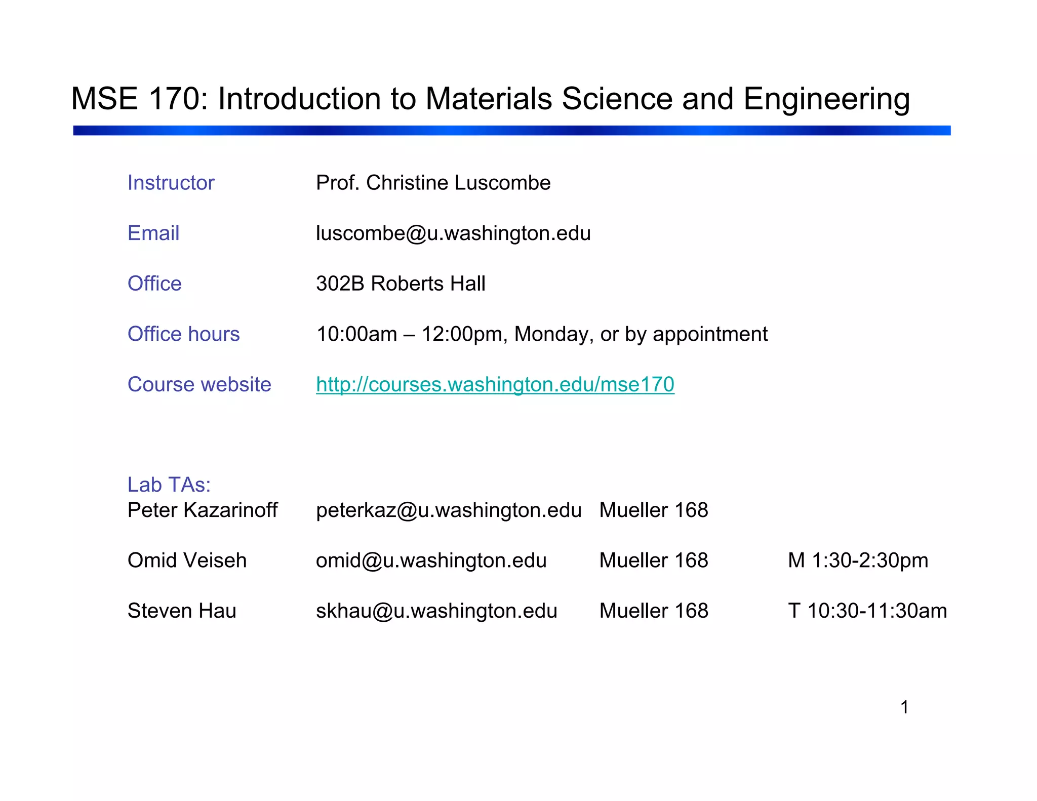
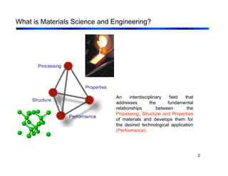


1. The document provides an overview of an introductory materials science and engineering course. It lists the instructor, their contact information, course website, and lab teaching assistants. 2. Materials are discussed through different historical ages from stone to modern materials like polymers and semiconductors. Key developments in processing and understanding of materials structures and properties are highlighted. 3. The document covers fundamental materials science topics like atomic structure, bonding, crystal structures, and how they influence materials properties. Different types of bonding and structures are compared.


