Download to read offline


![Solved with COMSOL Multiphysics 5.1
6 | S T R E S S E S A N D H E A T G E N E R A T I O N I N L A N D I N G G E A R
Application Library path: Multibody_Dynamics_Module/
Automotive_and_Aerospace/landing_gear
Modeling Instructions
From the File menu, choose New.
N E W
1 In the New window, click Model Wizard.
M O D E L W I Z A R D
1 In the Model Wizard window, click 2D.
2 In the Select physics tree, select Structural Mechanics>Multibody Dynamics (mbd).
3 Click Add.
4 In the Select physics tree, select Heat Transfer>Heat Transfer in Solids (ht).
5 Click Add.
6 Click Study.
7 In the Select study tree, select Preset Studies for Selected Physics Interfaces>Time
Dependent.
8 Click Done.
G L O B A L D E F I N I T I O N S
Parameters
1 On the Home toolbar, click Parameters.
2 In the Settings window for Parameters, locate the Parameters section.
3 In the table, enter the following settings:
Name Expression Value Description
m 5000[kg] 5000 kg Mass of the aircraft
vi 10[m/s] 10 m/s Downward velocity of
the aircraft
k_sa 2.5e6[N/m] 2.5E6 N/m Spring constant of
shock absorber](https://image.slidesharecdn.com/models-160106143141/85/Models-mbd-landing-gear5-1-6-320.jpg)
![Solved with COMSOL Multiphysics 5.1
7 | S T R E S S E S A N D H E A T G E N E R A T I O N I N L A N D I N G G E A R
If you do not want to build all the geometry, you can load the geometry sequence from
the stored model. In the Model Builder window, under Component 1 right-click
Geometry 1 and choose Insert Sequence from File. Browse to the application’s
Application Library folder and double-click the file landing_gear.mph. You can then
continue to the Add Material section below.
To build the geometry from a scratch, continue here.
G E O M E T R Y 1
Circle 1 (c1)
1 On the Geometry toolbar, click Primitives and choose Circle.
2 In the Settings window for Circle, locate the Size and Shape section.
3 In the Radius text field, type 0.15.
4 Locate the Position section. In the x text field, type -0.3.
Bézier Polygon 1 (b1)
1 On the Geometry toolbar, click Primitives and choose Bézier Polygon.
2 In the Settings window for Bézier Polygon, locate the Polygon Segments section.
3 Find the Added segments subsection. Click Add Linear.
4 Find the Control points subsection. In row 1, set x to -0.35.
5 In row 2, set x to -0.35.
6 In row 2, set y to 0.3.
7 Find the Added segments subsection. Click Add Linear.
8 Find the Control points subsection. In row 2, set x to -0.15.
9 In row 2, set y to 0.4.
10 Find the Added segments subsection. Click Add Linear.
11 Find the Control points subsection. In row 2, set x to -0.05.
12 Find the Added segments subsection. Click Add Linear.
c_sa 5e4[N*s/m] 5E4 N·s/m Damping coefficient of
shock absorber
k_t 2.5e7[N/m] 2.5E7 N/m Stiffness of tyre
c_t 2.5e6[N*s/m] 2.5E6 N·s/m Damping coefficient of
tyre
d 0.1[m] 0.1 m Out of plane dimension
Name Expression Value Description](https://image.slidesharecdn.com/models-160106143141/85/Models-mbd-landing-gear5-1-7-320.jpg)


![Solved with COMSOL Multiphysics 5.1
13 | S T R E S S E S A N D H E A T G E N E R A T I O N I N L A N D I N G G E A R
4 Select Boundaries 10 and 14 only.
Integration 2 (intop2)
1 On the Definitions toolbar, click Component Couplings and choose Integration.
2 In the Settings window for Integration, locate the Source Selection section.
3 From the Selection list, choose All domains.
Variables 1
1 On the Definitions toolbar, click Local Variables.
The heat generated due to the energy dissipation in the absorber is modeled as a
heat source. This heat source is distributed on the common boundaries of the
shock-absorber piston and cylinder.
2 In the Settings window for Variables, locate the Variables section.
3 In the table, enter the following settings:
H E A T TR A N S F E R I N S O L I D S ( H T )
Pair Boundary Heat Source 1
1 On the Physics toolbar, in the Boundary section, click Pairs and choose Pair Boundary
Heat Source.
2 In the Settings window for Pair Boundary Heat Source, locate the Pair Selection
section.
3 In the Pairs list, select Identity Pair 1 (ap1).
4 Locate the Boundary Heat Source section. Click the Overall heat transfer rate button.
5 In the Pb text field, type Q*1[m]/d.
Here, the total power is scaled with the actual out-of-plane thickness to get the
correct temperature distribution.
Name Expression Unit Description
Q mbd.prj1.Qdamper W Heat generated
per second
Wp intop2(mbd.rho*g_const*v*mbd.d) J Potential energy
h_sa timeint(0,t,Q) J Energy loss in
shock-absorber
Ws_sa mbd.prj1.Wspring J Energy stored in
shock-absorber](https://image.slidesharecdn.com/models-160106143141/85/Models-mbd-landing-gear5-1-13-320.jpg)


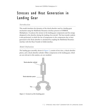
This model simulates the dynamics of a landing gear shock absorber during aircraft landing using COMSOL Multiphysics. It analyzes the stresses in the landing gear components and the heat generated in the shock absorber. The shock absorber piston and cylinder are connected by a prismatic joint with spring and damper elements. Springs and dampers also model the tire behavior. The model couples multibody dynamics, which calculates component stresses and displacements, with heat transfer analysis to determine temperature increases from shock absorber heat generation during landing.


