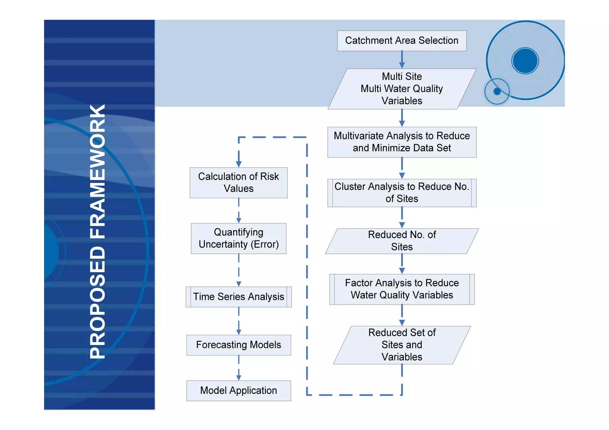
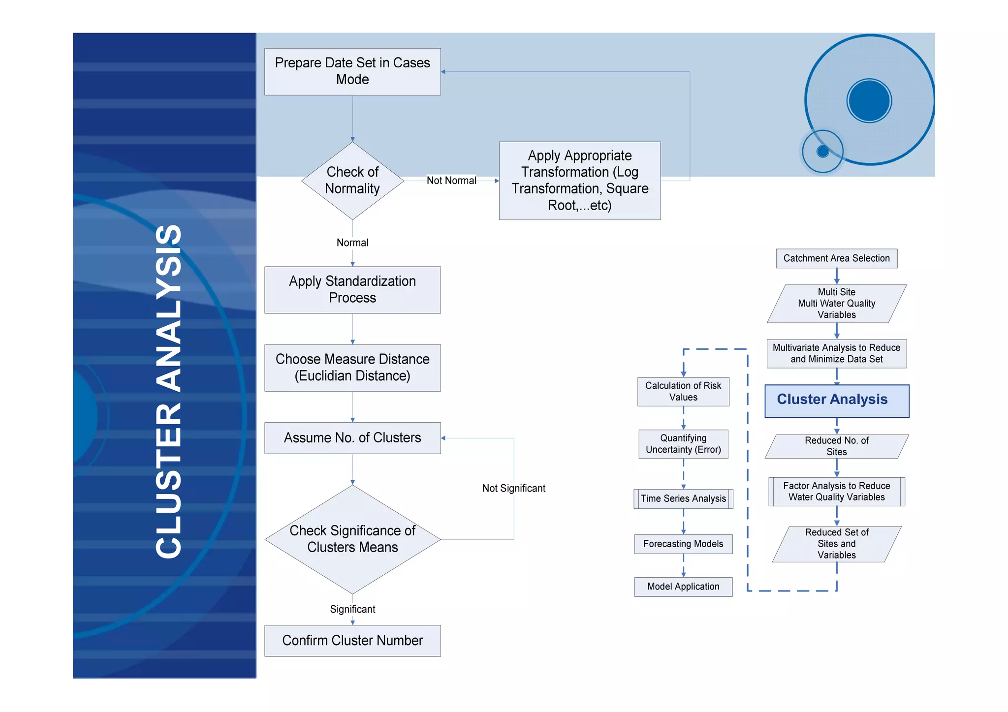
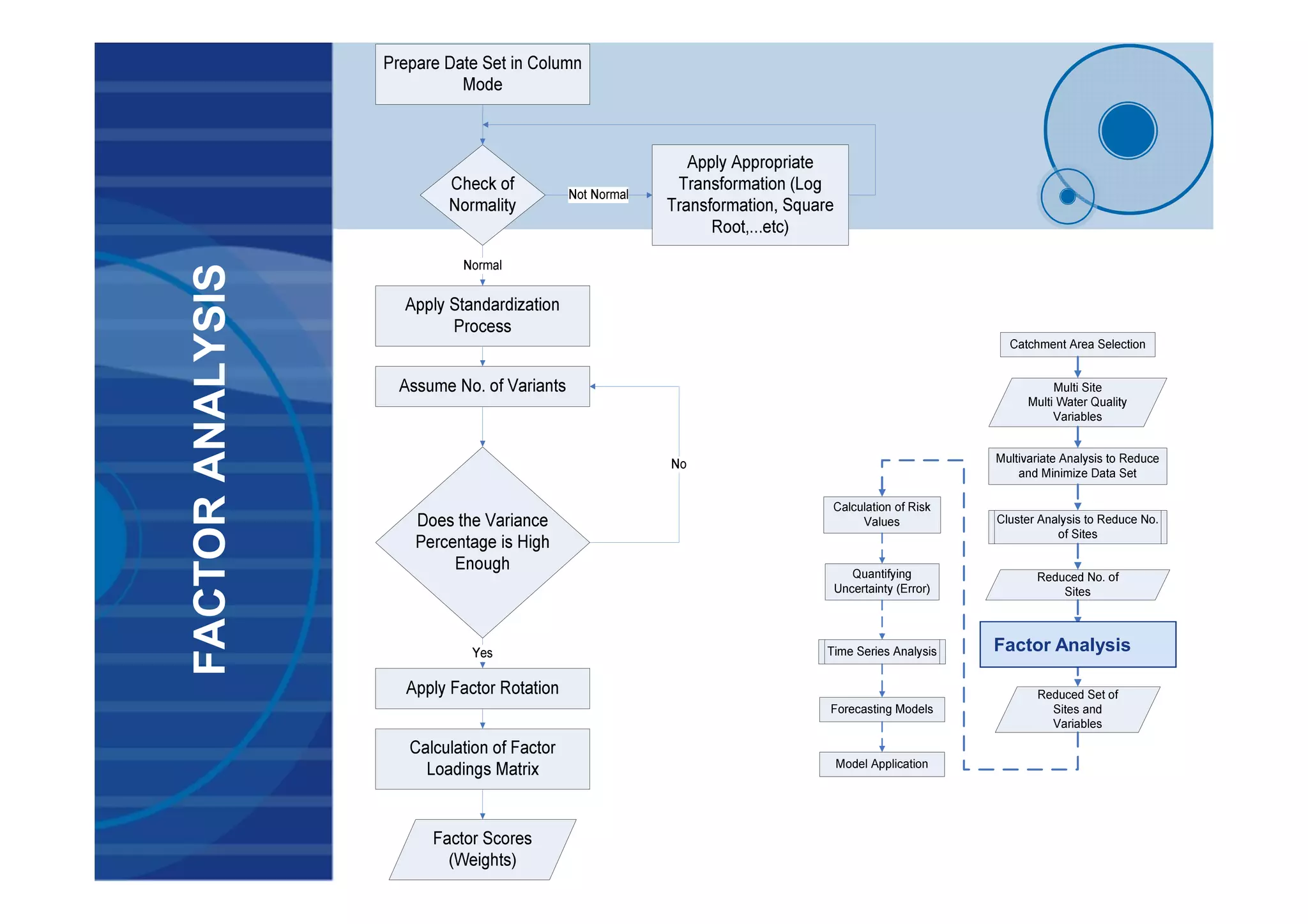
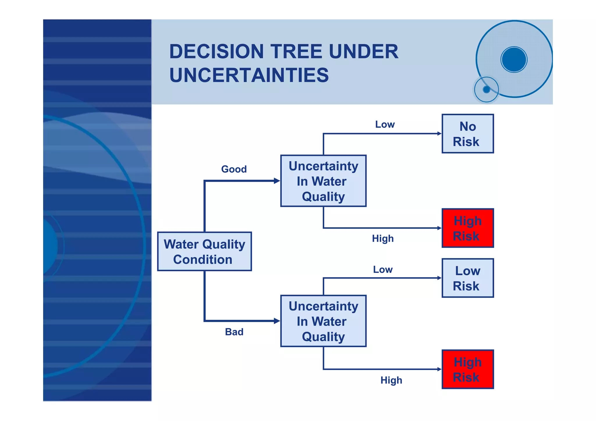
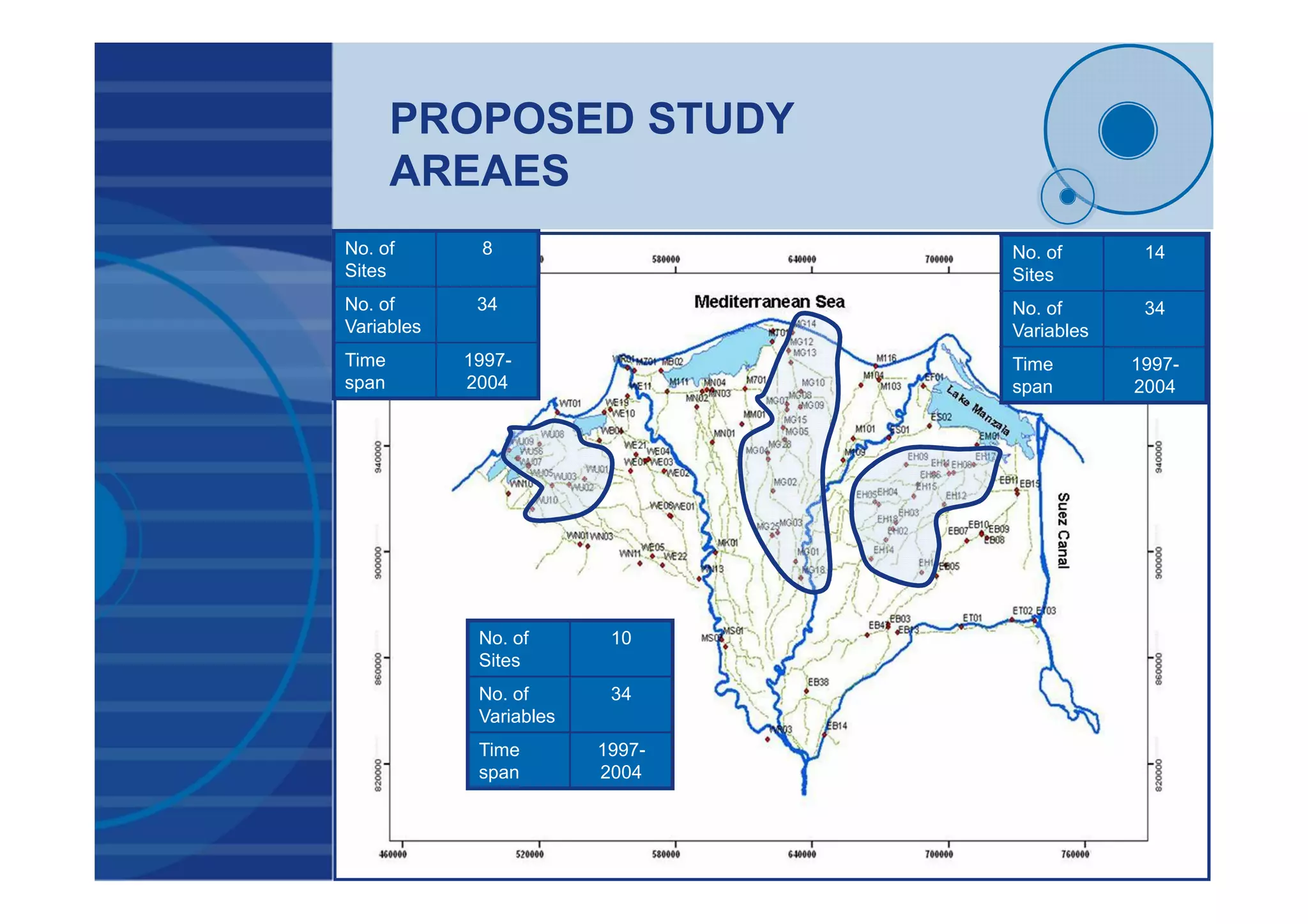
This document presents a probabilistic decision support system for water quality management that accounts for risk and uncertainty. It proposes a framework using cluster analysis to reduce monitoring points, factor analysis to construct water quality variants, and time series analysis of historical variant data. A decision tree is developed to classify water quality conditions and uncertainty levels, aiding management decisions. The framework was applied to 3 study areas in Egypt comprising 32 monitoring sites. Results demonstrated the approach for quantifying uncertainty and risk in variant time series to support probabilistic decision making under uncertain conditions.

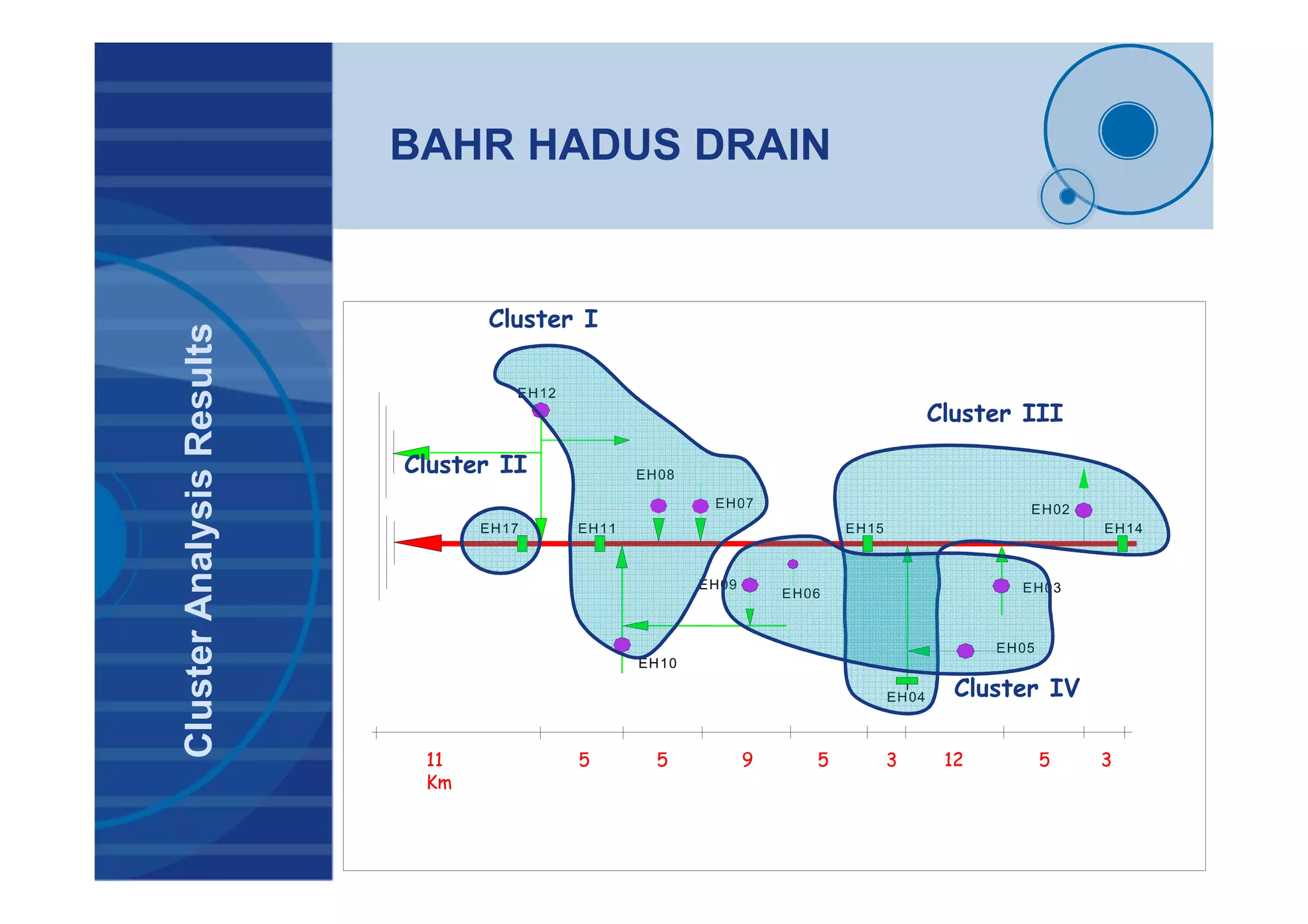
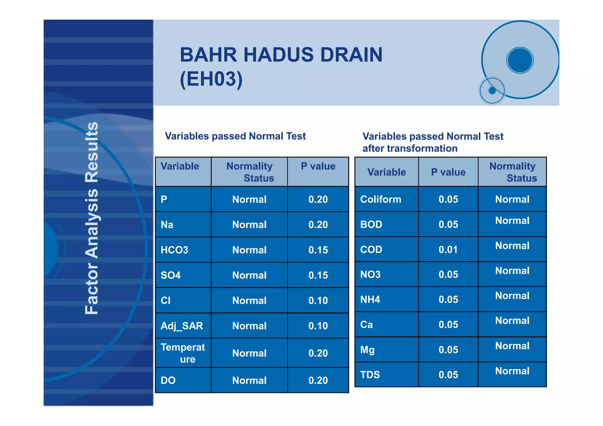
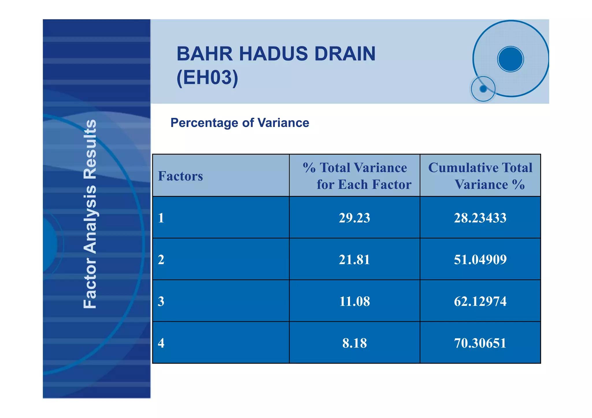
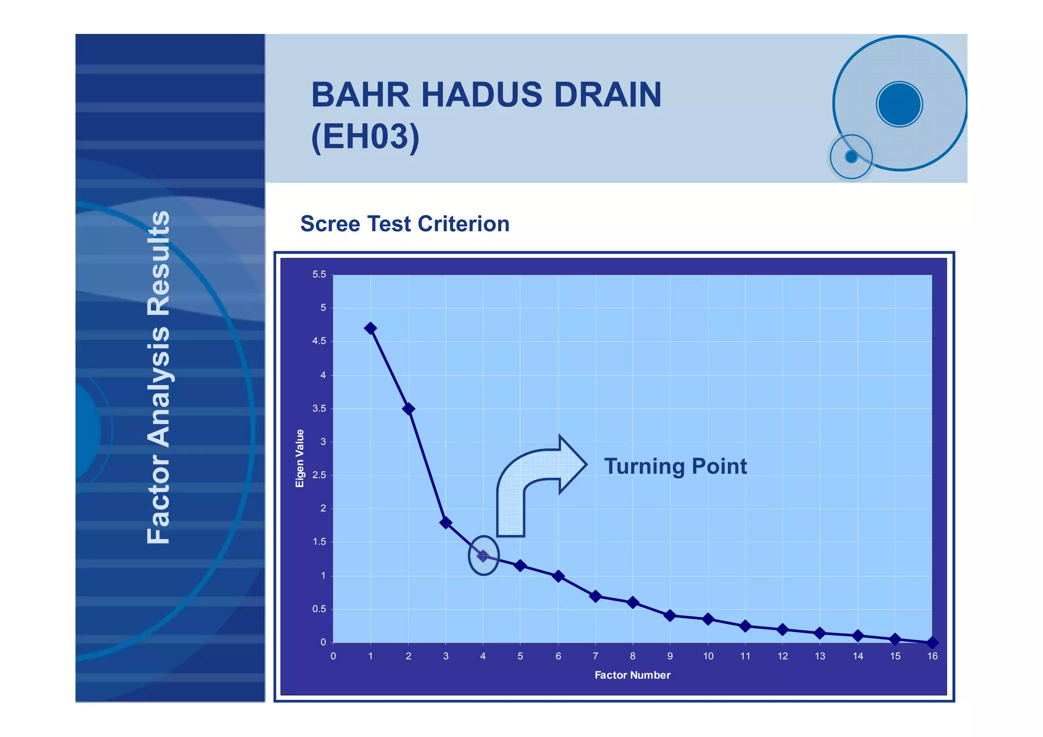
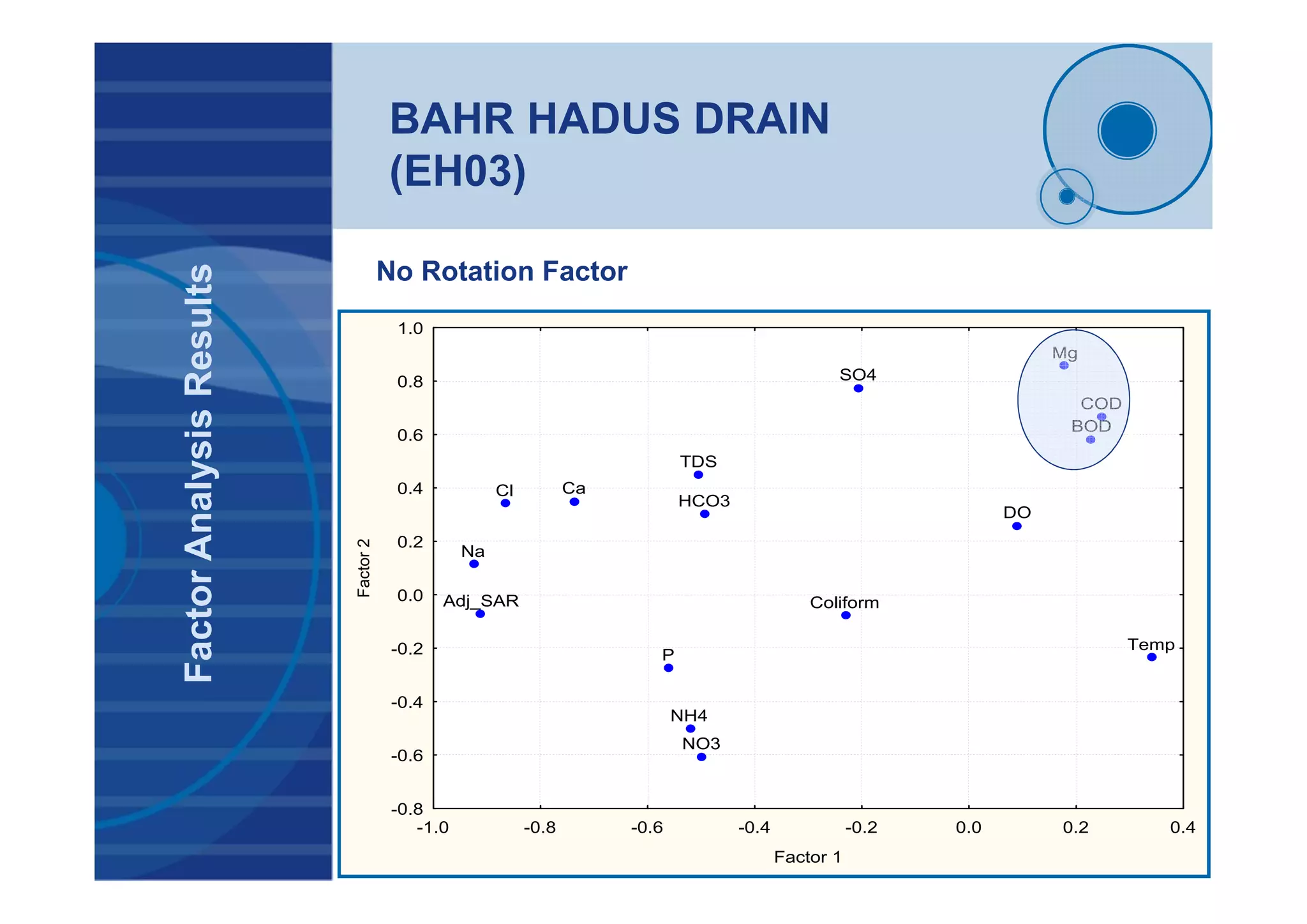
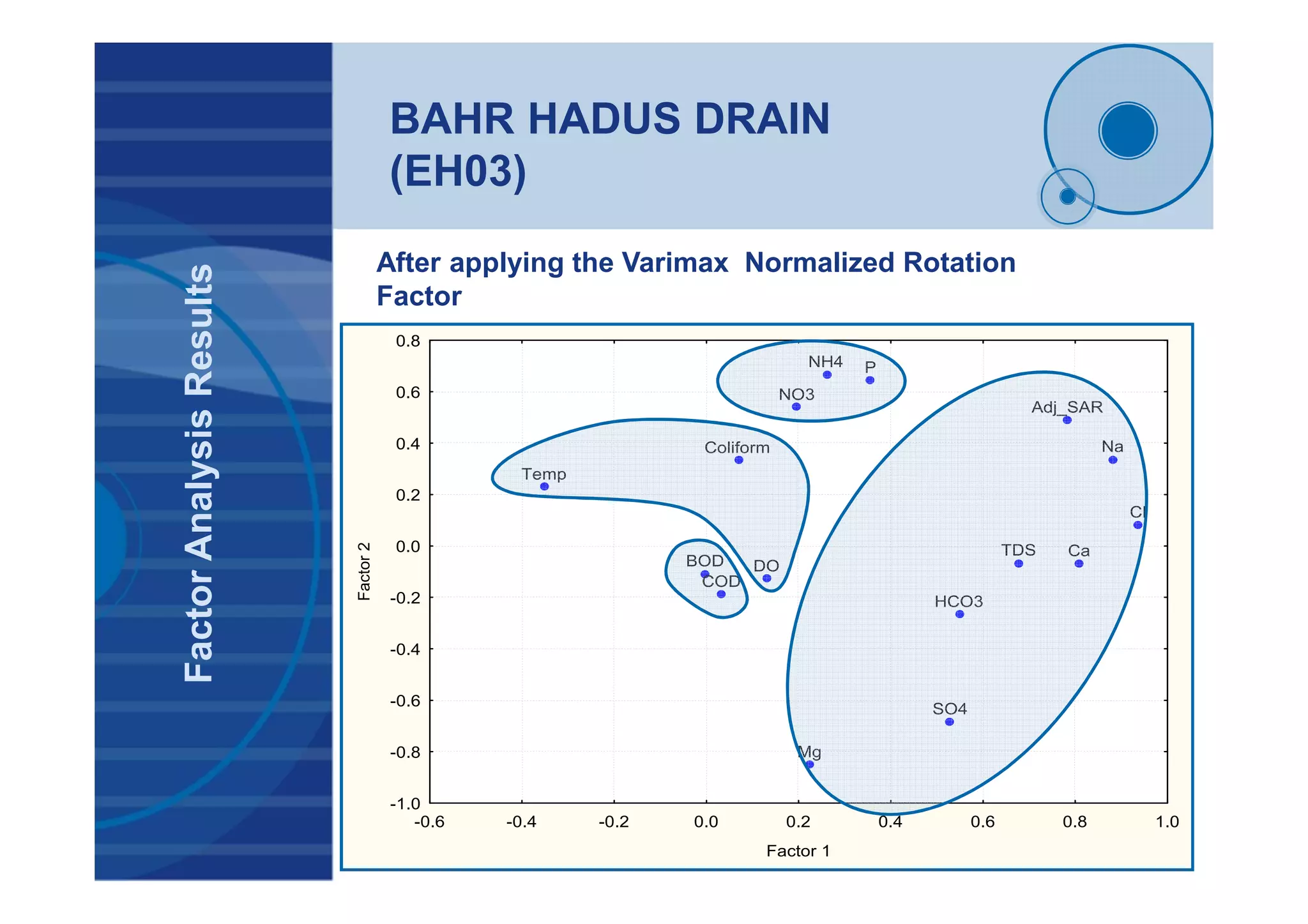
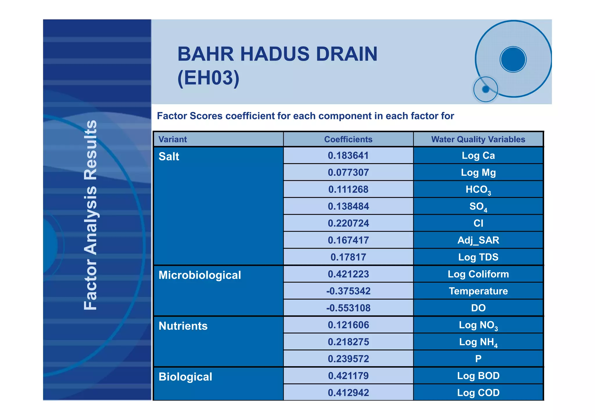
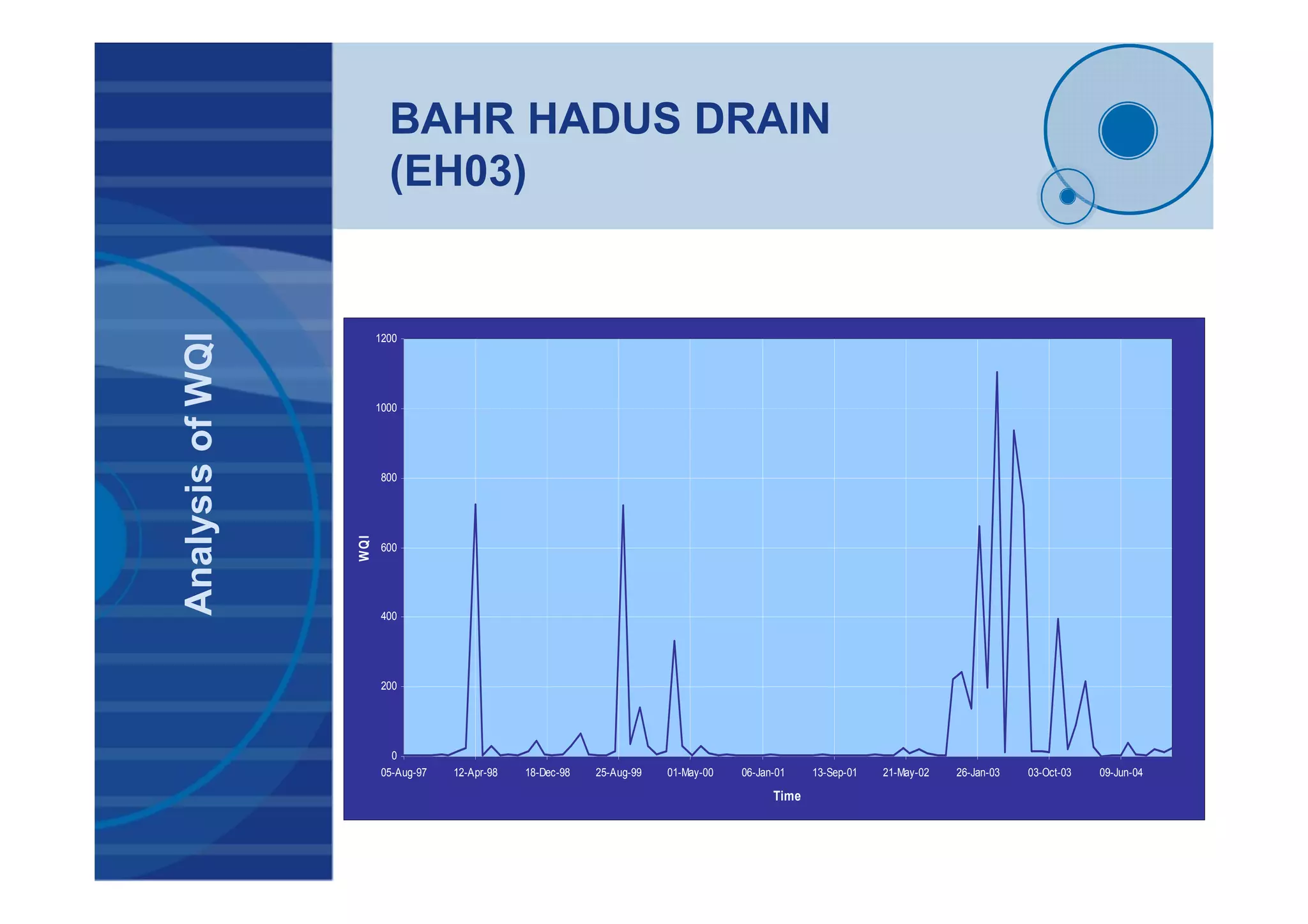
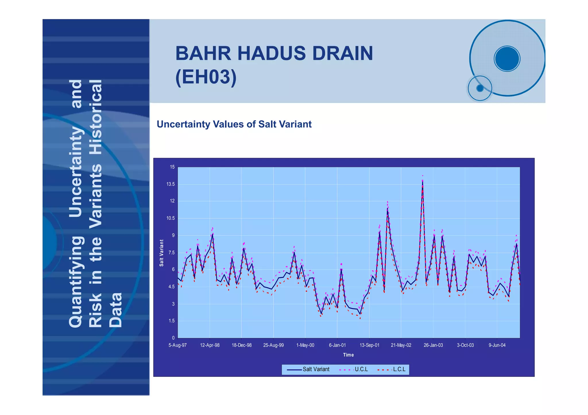
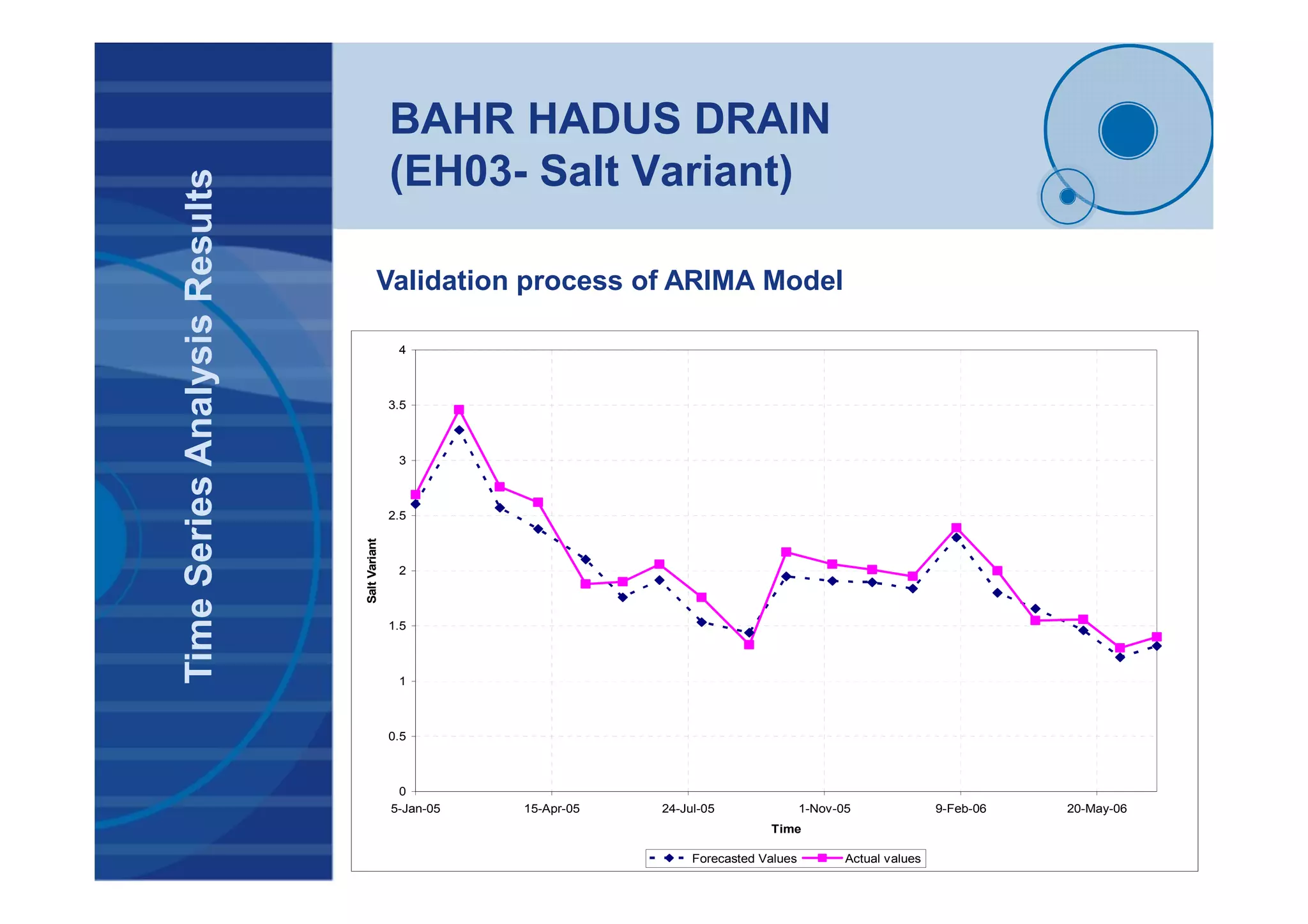
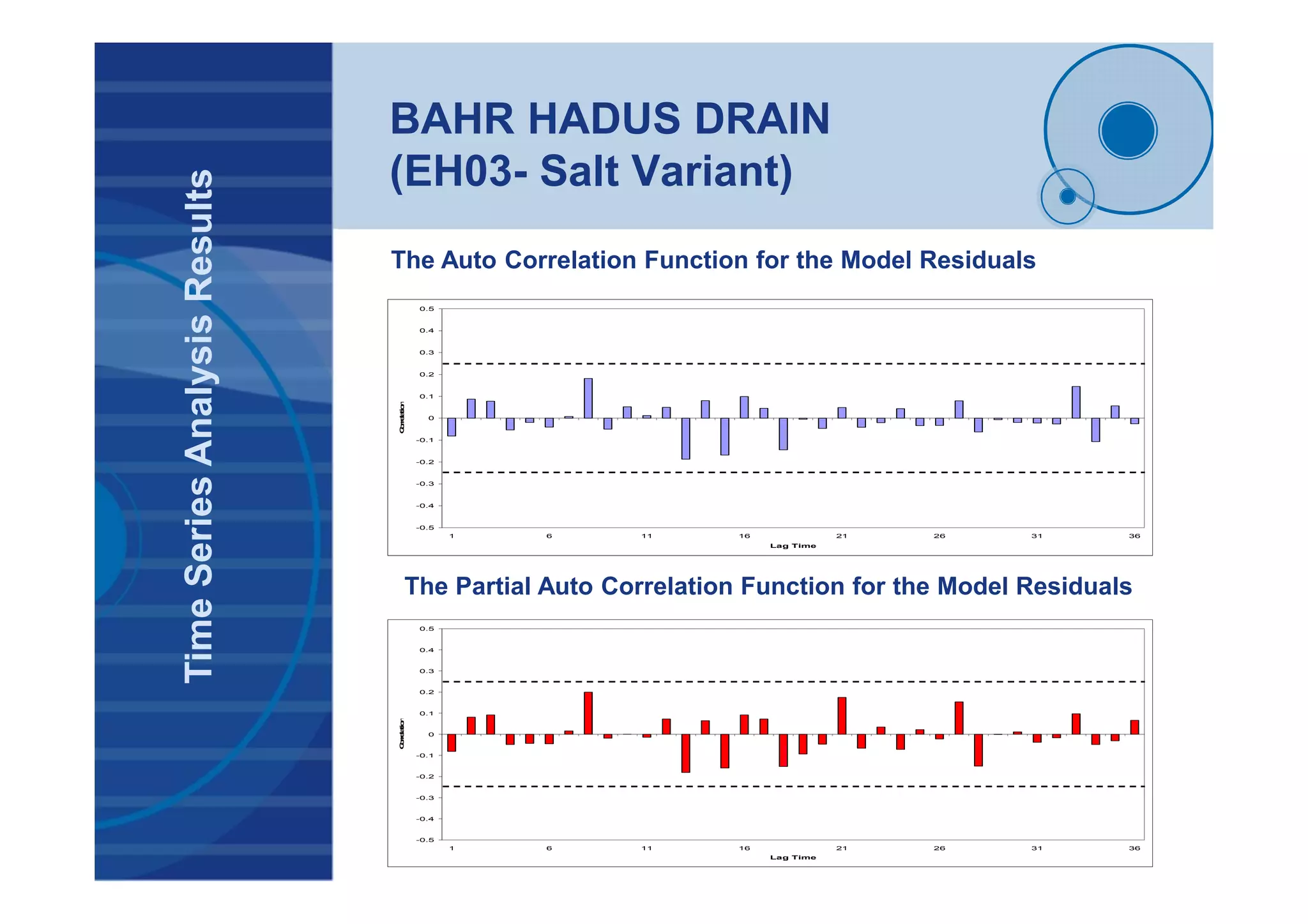
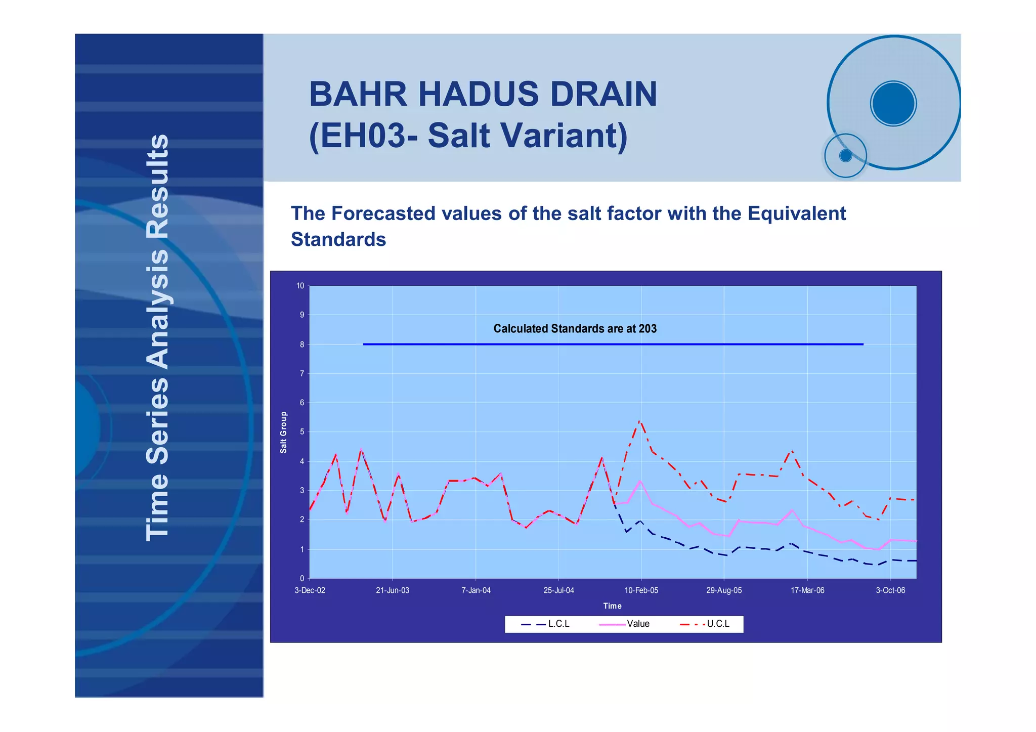
![BAHR HADUS DRAIN
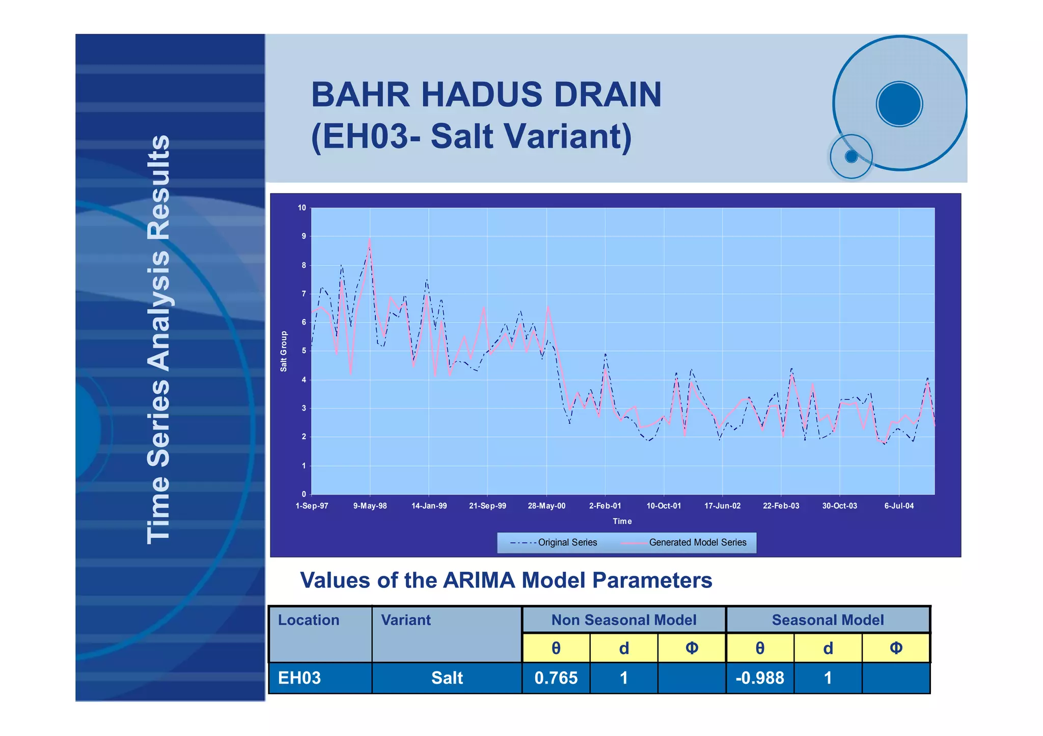
(EH03- Salt Variant)
TimeSeriesAnalysisResults
INFORMATION ON DIAGNOSTICS SELECTIVE ARIMA MODEL
SA quality index (stand to 10) 2.239 [0, 10] ad-hoc
STATISTICS ON RESIDUALS
Ljung-Box on residuals 15.87 [0, 33.90] 5%
Box-Pierce on residuals 00.44 [0, 5.990] 5%
Ljung-Box on squared residuals 24.89 [0, 33.90] 5%
Box-Pierce on squared residuals 00.09 [0, 5.990] 5%
Durbin-Watson statistic on residuals 2.16 [min:0, max:4]
DESCRIPTION OF RESIDUALS
Normality 1.30 [0, 5.99] 5%
Skewness 0.00 [-0.57, 0.57] 5%
Kurtosis 2.34 [1.87, 4.13] 5%
OUTLIERS
Percentage of outliers 2.33 % [0%, 5.0 %] ad-hoc
Results of the Statistical Tests Applied on the Residuals of
the Selected Model](https://image.slidesharecdn.com/31194138-c79c-4ee0-b028-6e0563b75dd2-160512182552/75/Phd-Presentation-47-2048.jpg)
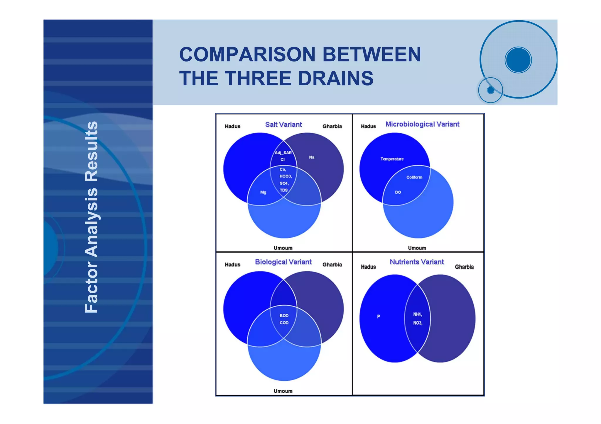
![COMPARISON BETWEEN
THE THREE DRAINS
TimeSeriesAnalysisResults
EH03 MG02 WU01
Salt Variant
[0,1,1][0,1,1] [1,1,1][1,1,1] [0,1,1][0,1,1]
Nutrients Variant
[0,1,1][0,1,1] [0,1,2][1,0,1]
Biological Variant
[1,1,1][1,0,1] [0,1,3][0,1,2] [0,1,1],[0,1,1]
Microbiological
Variant [1,0,0][0,1,1] [0,0,0][1,0,0]](https://image.slidesharecdn.com/31194138-c79c-4ee0-b028-6e0563b75dd2-160512182552/75/Phd-Presentation-52-2048.jpg)


![Lake Manzala Engineered Wetland, Port Said, Egypt [IWC4 Presentation]](https://cdn.slidesharecdn.com/ss_thumbnails/lake-manzala-engineered-wetland-port-said-egypt-iwc4-presentation2004-140821011400-phpapp02-thumbnail.jpg?width=640&height=640&fit=bounds)


